A new approach for sizing trials with composite binary endpoints using anticipated marginal values and accounting for the correlation between components
Abstract
Composite binary endpoints are increasingly used as primary endpoints in clinical trials. When designing a trial, it is crucial to determine the appropriate sample size for testing the statistical differences between treatment groups for the primary endpoint. As shown in this work, when using a composite binary endpoint to size a trial, one needs to specify the event rates and the effect sizes of the composite components as well as the correlation between them. In practice, the marginal parameters of the components can be obtained from previous studies or pilot trials, however, the correlation is often not previously reported and thus usually unknown. We first show that the sample size for composite binary endpoints is strongly dependent on the correlation and, second, that slight deviations in the prior information on the marginal parameters may result in underpowered trials for achieving the study objectives at a pre-specified significance level.
We propose a general strategy for calculating the required sample size when the correlation is not specified, and accounting for uncertainty in the marginal parameter values. We present the web platform CompARE to characterize composite endpoints and to calculate the sample size just as we propose in this paper. We evaluate the performance of the proposal with a simulation study, and illustrate it by means of a real case study using CompARE.
Keywords:
Composite Binary Endpoints , Correlated Endpoints , Sample Size.1 Introduction
Many trials are designed to evaluate more than one endpoint with the aim of providing a wider picture of the intervention effects [1, 2]. When the rate of occurrence of an event is expected to be low, it is common to consider the composite event defined as the occurrence of any of a set of pre-specified events. This composite event is usually chosen as the primary efficacy endpoint for comparing two treatment groups, either by comparing proportions between groups at the end of the study or by using time-to-event analysis. In this paper, we focus on composite binary endpoints.
Power analysis and its subsequent sample size calculation have been widely discussed in the literature on comparing two proportions in the univariate case [3, 4, 5, 6]. These standard sample size formulae are based on the effect size and the frequency of occurrence of primary endpoint, and they could be applied in a straightforward way to a composite endpoint if its effect size and frequency are known prior to the initiation of the study. However, the effect size and frequency of observing the composite endpoint depend on the corresponding effect and frequency of the composite components, which are often quite dissimilar and thus make the composite parameters very difficult to anticipate.
The TACTICS-TIMI trial [7] illustrates some problems that might arise when determining the sample size for a primary composite binary endpoint. TACTICS-TIMI 18 was an international, multicenter, randomized trial that evaluated the efficacy of invasive and conservative treatment strategies in patients with unstable angina or non-Q-wave acute myocardial infarction treated with tirofiban, heparin, and aspirin. The primary hypothesis of the TACTICS-TIMI 18 trial was that an early invasive strategy would reduce the combined incidence of death, acute myocardial infarction, and rehospitalization for acute coronary syndromes at six months when compared with an early conservative strategy. The primary endpoint was the composite endpoint formed by death, non-fatal myocardial infarction, and rehospitalization for acute coronary syndrome at 6 months.
Similar research questions such as those in TACTICS-TIMI 18 were previously investigated in the TIMI IIIB and VANQWISH trials[8]. The TIMI IIIB trial [9] considered the primary composite endpoint of death, post-randomization myocardial infarction, and a positive exercise test at 6 weeks; whereas the primary endpoint in the VANQWISH trial [10] was the combination of death and non-fatal myocardial infarction at 12 months of follow-up. The initial planning of TACTICS-TIMI was based on those trials expecting events of the primary composite endpoint in the conservative-strategy group, to detect a relative difference of between the two groups for a power. Those anticipated values resulted in the need to recruit at least patients. However, TACTICS-TIMI yielded a frequency of observing the combination of death, acute myocardial infarction and rehospitalization at six months, which was remarkably lower than expected and delivered a relative difference of between groups, a figure that is seriously lower than the anticipated . Note that if the anticipated frequency of observing the composite endpoint had been closer to the observed results, at least patients rather than would have been required and the sample size needed would have been larger than the one initially planned.
In this paper, we present sample size formulations for detecting a hypothesized difference between treatments in a primary composite binary endpoint based on the event rates and effect sizes of the composite components. The motivation for this is mainly because prior information on the marginal effects and event rates is commonly available from previous or pivotal studies, as illustrated in the TACTICS-TIMI trial. Moreover, the major findings in a trial with a primary composite endpoint should be well supported by its components [1, 11], since the trial could be considered negative if the components are not in line with the result [12, 13]. Nevertheless, as shown in this paper, the sample size calculation for composite endpoints relies not only on the anticipation of the effect size and the event rates of the composite components, but also on the correlation between them. However, even though the marginal parameters could be obtained previously, the correlation is usually not reported in practice and, thus, is frequently unknown and difficult to anticipate.
Several authors have addressed the correlation’s influence on sample size determination when more than one endpoint is used as the primary endpoint. Sozu et al. [14] discuss several methods for calculating power and sample size for multiple co-primary binary endpoints, and they study the impact on the sample size, specifically regarding the association among endpoints. Senn and Bretz[15] examine sample size for trials under different power definitions for multiple testing problems. Rauch and Kieser [16] and Sander et al. [17] define a multiple test procedure focused on a composite binary endpoint and a pre-specified main component, and propose an internal pilot study for estimating the unknown parameters and revising the sample size. However, to the best of our knowledge, methodologies are limited in regard to handling the sample size calculation for composite binary endpoints when the correlation is unknown.
The aim of this paper is two-fold. First, we focus on providing a general procedure for sizing trials with composite binary endpoints, doing so on the basis of anticipated information of the composite components even if the correlation is unknown. We show that the sample size for composite binary endpoints is strongly dependent on the correlation, and that slight deviations in the prior information on the marginal parameters may result in trials being too underpowered for achieving the study objectives at the pre-specified significance level. We propose a sample size strategy to calculate the minimum sample size that guarantees the planned power while accounting for, on the one hand, the uncertainty of the correlation value and, on the other, plausible deviations in the marginal parameter values. Second, we present CompARE, a freely available web-based tool for characterizing binary composite endpoints and computing the needed sample size under several settings. CompARE provides aids to help understand the role played by each one of the components of the composite endpoint, as well as their consequences on the required sample size. The methodologies presented in this paper have been implemented in CompARE.
This paper is structured as follows. In Section 2, we introduce the settings of the problem and the CompARE web tool. In Section 3, we review sample size planning when evaluating risk difference. In Section 4, we present sample size formulae for composite binary endpoints based on the parameters of the components plus the correlation. We further describe the performance of these formulae according to the parameters and propose a strategy for sizing trials when the correlation is unknown. In Section 5, we exemplify the proposal by the TACTICS-TIMI trial using CompARE, and in Section 6 we extend the proposal to those trials for which the treatment effect is measured by the relative risk or odds ratio. In Section 7, we investigate the performance of the power and significance level under misspecification of the correlation and evaluate the proposed sample size strategy with a simulation study. We conclude the paper with the Discussion.
2 Notation, assumptions and CompARE
We consider a randomized clinical trial comparing two treatment groups: the control group () and treatment group (), each one composed of patients who are followed for a pre-specified time . For simplicity, we consider only two events of potential interest, and . Let denote the response of the -th binary endpoint for the -th patient in the -th group of treatment (, , ). The response is defined by if the event, , has occurred during the follow-up and otherwise.
We define the binary composite endpoint as the event that occurs whenever one of the endpoints is observed, that is, . At this point we assume that the composite endpoint is well-defined, that is, both composite components are important enough to be considered; and we include those adverse clinical outcomes that are relevant to the clinical setting.
We denote by the composite response defined as a Bernoulli
random variable with probability of observing the event
, where:
| (1) |
To evaluate whether there is a risk reduction in the treatment group compared with the control group, we set a hypothesis test where the null hypothesis states that there is no difference between the control and the treatment groups; whereas the alternative hypothesis assumes a risk reduction in the treatment group. The usual measures to evaluate the treatment effect when comparing two groups are the difference in proportions (also called risk difference), denoted by ; the relative risk (or risk ratio), ; and the odds ratio, . The relationship between these measures and the probabilities of observing the binary composite endpoint in each group are given in Table 1, together with the null and alternative hypothesis that should be set in each case. The following sections will be developed in terms of the risk difference of the composite binary endpoint. Section 6 extends the results to the relative risk and odds ratio.
| Parameter Effect | Null hypothesis | Alternative hypothesis | |
|---|---|---|---|
| Risk difference | |||
| Relative risk | |||
| Odds ratio |
2.1 An insight into the parameters of the composite endpoint
Let and represent the probabilities that occurs or not, respectively, for a patient belonging to the -th group. Let denote Pearson’s correlation coefficient between the components in the -th group. The probability of observing the composite event is in terms of the probabilities of and and the correlation, as follows:
| (2) |
Note here that the probability of observing the composite endpoint becomes smaller as the correlation between the components of the composite increases.
The effect size in the composite endpoint in terms of the risk difference, , is given by:
| (3) |
where () corresponds to the risk difference for each of its components.
From now on the correlation is assumed equal for both groups and denoted by , that is, . Let denote the vector of event rates of the composite components in the control group, that is, , and let represent the vector of marginal effect sizes, that is, . We will denote the risk difference as a function of the marginal parameters () and the correlation by ; and the probability of observing under the control group by . We remark here that when and are fixed such that and (), the risk difference increases with respect to the correlation (see Appendix A).
2.2 CompARE
We present CompARE11 1 Link to CompARE: https://cinna.upc.edu/compare/, the open-source code for CompARE is available at: https://github.com/MartaBofillRoig/CompARE, an open-source and completely free web platform that can be used as a tool for clinicians, medical researchers and statisticians to compute the sample size according to the procedure proposed in this paper. Furthermore, CompARE can be used to:
- 1.
Determine the sample size for different situations, among them, when the correlation is not known.
- 2.
Specify the treatment effect for the composite endpoint based on the marginal information of the composite components, and to study the performance of the composite parameters according to them.
- 3.
Calculate and interpret the measures of association among the composite components, then investigate their characteristics.
- 4.
Figure 1 summarizes all the capabilities of CompARE. To use CompARE, the least you should provide is the effect size and event rates of the composite components as well as the correlation.

3 Sample Size when the parameters of the composite endpoint can be anticipated
In this section we summarize the statistics and sample size formulae to test for a risk difference when the probability of occurrence in the control group of the composite binary endpoint can be anticipated and for a given expected risk difference. Since the composite endpoint is an univariate outcome, a single statistical test is performed and, consequently, no multiplicity problem occurs and no statistical adjustment is needed. Therefore, as we will see, the formulas follow the univariate case and are straightforward but to make the paper comprehensive and the following sections meaningful, we displayed them in terms of the composite endpoint parameters.
Herein we assume a clinical trial where, first, patients are randomized to one of two treatment arms following a balanced design and, second, where the primary endpoint is a binary composite endpoint. The aim is to detect a hypothesized risk reduction in the primary composite endpoint at the significance level of and with desired power equal to . Let be the total sample size required, with patients per group (); and let us denote by and the values of standardized normal deviates corresponding to and .
The null hypothesis is stated as and is compared against the alternative hypothesis . To test against we use the statistic:
| (4) |
where . Under , follows, asymptotically, the standard normal distribution. We will reject the null hypothesis at the level of significance if . The variance in equation (4) can be estimated under using the pooled variance estimate[4]:
or under using the unpooled variance estimate:
4 Sample Size based on anticipated values of the composite components
Sample size formulae underlined in Section 3 are based on the parameters of the composite endpoint, that is, the event rate under the control group, , and the treatment effect, . In this section, we derive the sample size based on the anticipated information on the marginal parameter values and the correlation, even if the correlation value is not fully specified and/or the event rates values are not accurately anticipated.
4.1 Sample size based on composite components
Given the event rates in the control group , the expected effect size for each component , and the correlation between the occurrence of both components , we will denote by the needed sample size, which is computed by using the unpooled variance estimate, to detect a risk difference (see equation (3)) at significance level with power.
The expression for is obtained after direct substitution into formula (6) and is as follows:
| (7) |
where is given in (2). Note that the sample size also relies on the significance level and the power , but these are omitted for ease of notation. The corresponding sample size under the pooled estimate can be analogously calculated by using , and and its expression can be found in the online support material.
4.2 Sample size bounds
Assuming that the correlation is the same in the two treatment groups, it follows that the correlation takes values between the lower bound, , and the upper bound, , which are functions of and , and are defined as:
| (8) | |||||
Note that when at least one of the event rates is very close to , the lower bound will also be close to and the plausible correlation values will be always positive. We also notice that, in clinical trials the probabilities of observing the events are often quite low and commonly smaller than . In this case, the expressions for and can be simplified. See the online supplementary material for more details.
Considering such bounds for a given marginal parameters and , the sample size is an increasing function of the correlation , and it is bounded below and above by and , respectively. As a consequence, the more correlated the single endpoints are, the larger will be the necessary sample size for detecting the differences between groups in the composite endpoint. Details for this derivation are provided in Appendix B (see Theorem 1).
4.3 Sample size with uncertain correlation value
Since the correlation plays an important role in calculating the sample size, we propose a strategy for deriving the sample size when the parameters that correspond to the composite components are known and the correlation value is not specified in advance.
Prior knowledge about the effect of the treatment being investigated can lead to scientists foreseeing whether the two events of interest, and , are weakly, moderately or strongly correlated. We allow for prior information by splitting the rank of the correlation into three equal-sized intervals, and we consider three correlations categories: weak for the interval whose correlation values are lower; moderate for those intermediate correlation values; and strong for those correlation values that are higher. If any information exists, we will take it into account and will proceed as follows:
- (i)
Correlation bounds for each category:
Considering the categories weak/moderate/strong for the correlation, the plausible correlation values for a given () are in this situation those between the lower and upper values within each category. If the events are weakly correlated, the correlation is between and ; if they are moderately correlated, its value lies between and ; and if they are strongly correlated, it is between and .
If we cannot place the correlation in any of the above categories, we use the most severe case within its plausible values, then, . (See Table 2). - (ii)
Calculate the sample size in each category:
For the sample size, we advocate using the maximum sample size across all its possible values. That is, , , and for weak, moderate or strong correlations, respectively. Note that since we are assuming the correlation value that maximizes the sample size across its plausible values, we are guaranteeing that the pre-specified power is attained.
If the correlation value can not be ascribed to any category, then, we propose a conservative sample size strategy of using the overall possible maximum sample size, that is, . Table 2 outlines the range of correlations and sample sizes values, together with the proposed sample size for each category.
| Category | Correlation Bounds | Sample Size Bounds | Sample Size |
|---|---|---|---|
| Weak | |||
| Moderate | |||
| Strong | |||
| No prior information |
4.4 Sample size accounting for departures from the anticipated event rates
The marginal parameters are often estimated through previous studies or pivotal trials with a limited number of patients and whose patient populations or concomitant drugs could differ from the current ones. Because of that, there is great uncertainty in the values that need to be anticipated for computing the sample size. In this section, we consider that the event rates and have been previously estimated and their corresponding standard errors of the point estimate are provided.
Let denote a set of plausible values for the true value of . For instance, for those previous trials in which we have the standard deviations for the event rates, we can use the set of plausible values for that a confidence interval would yield. We address the issue of sizing a trial for a significance level and power based on the intervals and , and for fixed effects and when the correlation value is not known.
We state that, for given and and at fixed , the sample size (see equation (7)) that is needed for power at a significance level , falls into the interval:
| (9) |
This interval is such that it contains the sample size required to attain power , which is necessary for detecting an effect size equal to at a significance level according to the marginal effects and , the correlation , and the event rates within (). Note that the interval gives us the plausible sample size values by taking into account the uncertainty of the marginal parameter values, and it provides us the maximum sample size that we would need even though the anticipated event rates are not accurate.
Considering the set of values for the marginal parameters, and denoting by and the lower and upper bounds of the correlation within the set . Then, for all , and , we have that:
| (10) |
Furthermore, for given , the sample size is an increasing function of the correlation .
The sample size given by delimits the values that the sample size could have in terms of the correlation accounting for plausible deviations in the anticipated event rates. If there is no prior information on the correlation, we can use as the needed sample size. If otherwise, we have some prior information on the correlation value, the rationale used in 4.3 using correlation categories can be as well applied here to the function . Table 3 provides the sample size strategy under this circumstance. We lay out the performance of the sample size when varying the event rates in the intervals and and the subsequent sample size behavior according to the correlation in Propositions 2 and 3 in the supplementary material.
| Category | Correlation Bounds | Sample Size Bounds | Chosen Sample Size |
|---|---|---|---|
| Weak | |||
| Moderate | |||
| Strong | |||
| No prior information |
4.5 Power performance of the proposed strategies
Given () and for a fixed sample size , the power function using the unpooled variance estimate is defined as:
| (11) |
where denotes the cumulative distribution of the standard normal distribution. The power function for the pooled variance estimator can be found in the online support material.
In what follows, we show that the planned power is achieved with any of the previous strategies in Subsections 4.3 and 4.4.
- 1.
If and are fixed and the correlation value is not known, we have and the proposed sample size becomes . The resulting power is then such that:
The power attained using the upper bound of the correlation is equal to the pre-specified power value () when the correlation is the maximum value within its range, that is, . Otherwise, if the correlation is less than , the power will be always higher than the pre-specified power. Table S1 in the online supplementary material details the power performance when the correlation categories are taken into account.
- 2.
If the event rate value is within the interval for and the effect sizes are fixed, then . If in addition we have no prior information on the correlation value, then since the sample size increases with respect to the correlation, it follows that , and then the proposed sample size turns into . The corresponding power then satisfies:
The power attained is equal to the pre-specified power value when the event rates take the upper values and the correlation is equal to . If that is not the case, the power obtained will be larger than the pre-specified .
5 Motivating example: TACTICS-TIMI trial
In managing the syndrome of unstable angina and non-Q-wave acute myocardial infarction, there is controversy over whether using an invasive strategy rather than a conservative strategy offers any advantage. TACTICS-TIMI was a randomized trial that evaluated the efficacy of invasive and conservative treatment strategies in patients with unstable angina and non-Q-wave AMI treated with tirofiban, heparin, and aspirin [7].
Patients were randomly assigned to either an early invasive strategy or an early conservative strategy. The primary hypothesis of the TACTICS-TIMI trial was that an early invasive strategy would reduce the combined incidence of death, acute myocardial infarction, and rehospitalization for acute coronary syndromes at six months when compared with an early conservative strategy. The primary endpoint was the composite endpoint formed by a combination of incidence of death or non-fatal myocardial infarction (), and rehospitalization for acute coronary syndrome () at six months.
For illustrative purposes, we assume that a trial will be planned for a similar setting and that the results of TACTICS-TIMI 18 are to be used. Since previous studies to TACTICS-TIMI 18 also considered the events death and non-fatal myocardial infarction altogether, we presume that the event rate and effect size on the endpoint can be anticipated despite being composed by two events. The estimated values for the frequency of death or non-fatal myocardial infarction () in the conservative strategy group was with a standard deviation of ; whereas the frequency of rehospitalization for acute coronary syndrome () was with a standard deviation of . Based on the standard deviations of the estimated event rates, we use the confidence intervals as a set of plausible values among which the true values , take values, that is, and . The observed effects on TACTICS-TIMI were and , and we will use these as the expected effects on the new experimental trial.
We consider these parameters to construct the correlation bounds outlined in equation (8). The effects and and the values and imply that the eligible values for lie in the interval (, ). Using the intervals and , the correlation bounds are such that the considered values are plausible for any event rate within and . This gives us the correlation bounds (, ). Table 4 and its accompanying figure show the correlation bound according to and with varying values of the event rates. Observe that the upper bound takes the value when both event rates are equal, and the lower bound tends to when at least one of the event rates becomes smaller.
![[Uncaptioned image]](1807.01305v2/CorrelationPlot.png)
| Event rate values | Correlation Bounds |
|---|---|
| , | |
| , | |
| , |
FIGURE Lower bound (surface in blue) and upper bound (in red) for the correlation according to the effect sizes , and where the marginal event rates take values between and .
We illustrate the aspects of calculating power and sample size using the platform CompARE. CompARE calculates the sample size by anticipating the marginal information in terms of either risk difference, relative risk, or odds ratio. In this particular case, we use the statistical test for risk difference under pooled variance in order to ascertain the treatment differences in the composite endpoint at a significance level of and target power of . The results obtained from CompARE are presented in the form of summary tables and plots.
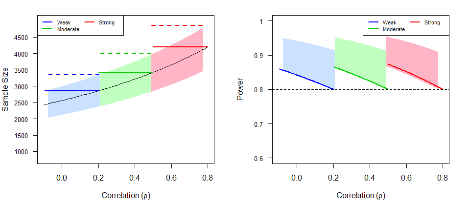
Figure 2 (left panel) depicts the performance of the sample size in terms of the correlation for given marginal parameters and ; and it illustrates the recommended sample size for each correlation category (weak, moderate, and strong). The solid line represents the sample size as a function of the correlation computed for the anticipated values , and the shaded areas represent the region of values, constructed by , , and , within which interval the sample size falls. Based on and the proposed sample size (in dotted lines) is the upper value of the shaded area within the correlation category.
Note that the sample size is highly sensitive to the anticipated parameters. For instance, for , using and , the required sample size is . This sample size, however, can differ substantially from that calculated using other reasonable values, such as the upper or lower limits for the intervals and , which would imply and , respectively.
Figure 2 (right panel) describes the statistical power achieved under the proposed method. Assuming that we have correctly anticipated the correlation category, observe that in all cases the achieved power is larger than the planned power, . Then, the method guarantees the desired power. If we could correctly anticipate the values of the event rates, then the achieved power would lie between and , in accordance with the plausible correlation values. If we base the sample size calculation on the intervals and , we will be overestimating the statistical power more than in the previous case, thus obtaining a power between and .
Table 5 describes the proposed sample size for each correlation category and reports the possible values for the statistical power, assuming that we have correctly anticipated the correlation category.
| Based on point values , for the event rates: | |||
| Correlation bounds: , . | |||
| Association strength | Correlation | Sample size | Achieved power |
| Weak | (, ) | ||
| Moderate | (, ) | ||
| Strong | (,) | ||
| Based on intervals and for the event rates: | |||
| Correlation bounds: , . | |||
| Association strength | Correlation | Sample size | Achieved power |
| Weak | (, ) | ||
| Moderate | (, ) | ||
| Strong | (, ) | ||
6 An extension for risk ratio and odds ratio
In this Section, we show that the risk ratio and odds ratio for the composite endpoint can also be expressed in terms of its margins plus the correlation, and we extend the sample size derivation given in Section 4 for evaluating the risk and odds ratio.
6.1 Composite effect expressed in terms of the risk ratio or the odds ratio
Let and denote the risk ratio and odds ratio, respectively, for the -th event. The risk ratio for the composite endpoint, , is expressed in terms of the risk ratio of its components and , the event rates under control group, and , and the correlation between them, , as follows:
| (12) |
Analogously, the odds ratio for the composite endpoint is defined according to its margins and the correlation is given by:
| (13) |
The derivations of equations (12) and (13) are postponed to Appendix A. By inspection of (3), (12), and (13), we observe that if there is no effect on the components, that is, , or , then there is no effect on the composite endpoint, . However, the reciprocal does not follow: no effect on the composite endpoint is compatible with some effect on the components. Therefore, it is important to remark, as other authors have warned before [21, 22, 23], that not finding a beneficial effect on composite endpoint is not a guarantee of not having some effect on the components, hence the effect on the composite endpoint cannot be treated as if it were an indicator of some specific effect on its components.
6.2 Sample size calculations in terms of risk ratio and odds ratio
The null hypothesis in terms of the risk ratio is stated as and the alternative hypothesis assuming a risk reduction is . The statistic that we use for testing the significance of the relative risk R∗ is:
where . Under , asymptotically follows the standard normal distribution; thus, we will reject at the significance level if . As in Section 3, we estimate the variance using the pooled variance by means of or by using the unpooled variance, .
For a given probability under control group , and a significance level , the needed sample size for detecting a risk ratio with power is given by:
| (14) |
The corresponding sample size when the pooled variance is used can be seen in Table 6.
When measuring the effect of treatment with the odds ratio, the null hypothesis is compared with the alternative hypothesis . To test the above hypotheses we use the statistic:
where and where the pooled and unpooled variance estimates are given, respectively, by and .
Then the needed sample size is calculated using the unpooled variance, for detecting a treatment difference of in order to have power at level for given , and it is given by:
| (15) |
The sample size expression when using the pooled variance can be found in Table 6.
| Variance estimator | Sample Size formula | |
|---|---|---|
| Risk difference | ||
| Pooled variance | ||
| Unpooled variance | ||
| Risk ratio | ||
| Pooled variance | ||
| Unpooled variance | ||
| Odds ratio | ||
| Pooled variance | ||
| Unpooled variance |
-
where: and .
6.3 Sample size derivation based on its margins
Analogously to Section 4 and following the notation in Section 4.4,, we obtain the sample size based on the risk ratio as a function of the marginal effects and , the event rates , and the correlation . To do so, we take the event rate and risk ratio of the composite endpoint for their expressions (which are defined according to , , and , see equations (2) and (12)), and then substitute these into the sample size formula in (14). We denote by the needed sample size for evaluating the risk ratio computed for specific values , , and . We will analogously proceed with sample size in terms of the odds ratio using the effects and , then denote by the corresponding sample size.
In what follows, we describe the performance of the sample size when the effect is measured by odds ratio or risk ratio. Further details of these properties and their empirical proof are to be found in the web supplementary material.
- 1.
For fixed () or (), the sample size for testing the effect measured by the risk ratio, , and the sample size for testing the odds ratio, , are increasing functions of the correlation .
- 2.
For given and at fixed , the needed sample size to have power at a significance level falls into the interval:
(16) Analogously, for given and , the needed sample size lies within the interval:
- 3.
For all and , it follows that:
Furthermore, for given () or (), the sample size functions and increase with respect to the correlation .
Note that, unlike when using risk differences, the sample size has its maximum value when both event rates take their lower interval values (see equations (9) and (16)).
Also note that if the marginal parameters () or () are anticipated and the correlation is not known, the sample size strategy described in Section 4.3 can be extended to the risk and odds ratio and analogously applied. For fixed effects () or (), and given intervals and for the event rates, we can follow the same reasoning as for risk differences in Section 4.4, and use (analogously ) to calculate the required sample size that guarantees the planned power while accounting for the unknown correlation value and uncertainty of the marginal parameter values.
7 A simulation study
We conduct a simulation study to evaluate the strategies proposed in Section 4 for computing the sample size.
7.1 Design
We simulate a two-arm trial with a composite primary endpoint composed of two events, and , according to the following values (which are all summarized in Table 7): the marginal probabilities of observing ( in the control group take values between and , and they are without loss of generality such that ; the risk ratios are specified for beneficial effects and vary from to ; the true correlation between and is assumed to be common for both groups, and it covers the positive range between and . The possible combinations add up to a total of 421 different scenarios which take into account that for given . simulations are performed only for those between and (see (8)).
For each one of these 421 scenarios specified by (, , ), we compute the required sample size for a one-sided test with power at the significance level , which is done by following one of the six different formulations that are derived in Section 3 and Section 6 and, additionally, are all summarized in Table 6.
We distinguish 4 different situations according to the value we assume in to calculate :
- 1.
For the weak correlation category, use
- 2.
For the moderate correlation category, use
- 3.
For the strong correlation category, use
- 4.
For guessing the true correlation, use .
Given one scenario specified by (, , ), we evaluate the type I error first by calculating based on and simulating trials using ). To check the power, we start by calculating as above, based on , and then we simulate trials using ). Altogether, we have to analyze a total of 3368 scenarios.
The above steps have to be reproduced six times according to the different sample size formulae used to compute , that is, by stating the effect in terms of the difference in proportions, the risk ratios or the odds ratio, and using both the pooled and the unpooled estimates of the variance. We have performed all computations using the R software tool (Version 0.98.1087), and the time required to perform the considered simulations was 55.58h.
| Parameter | Values |
|---|---|
| Effects used to evaluate the power: | |
| Effect used to evaluate the type I error: | |
7.2 Power analysis of the proposed strategies for computing sample size
Let be the required sample size calculated using the formulae described in Table 6 where , indicating whether the pooled or unpooled variance has been used; and , indicating the effect measure that has been tested. In other words, for the difference in proportions, ; for relative risk, ; and for odds ratio, . Let denote the empirical power when the total number of participants is (; ).
Whenever the correlation we are using to compute the sample size coincides with the one we have used to run the simulations (), the empirical powers are always achieved whether we are using the pooled, , or unpooled, , estimator of the variance. Nevertheless, when testing the difference in proportions, the achieved powers do not substantially differ (); when testing the treatment differences in terms of the risk ratio or the odds ratio, the power achieved if the unpooled variance estimator is used is slightly larger than the power achieved with the pooled estimator, , (see Table S3 in supplementary material for a comparison of the two approaches). The results presented herein refer to the unpooled variance estimator. The corresponding results for the pooled variance are summarized in the supplementary material (Table S4 and Figure S1).
When , we distinguish two types of misspecification. Misspecification type I, and pertain to the same correlation category; and Misspecification type II, and do not belong to the same category. Table 8 describes the empirical power in these two cases, which account for the correlation category for the three effect measures that we could use to test the difference between groups. If Misspecification I occurs, the pre-specified power is achieved and might exceed .
For misspecification II, there are two possible scenarios. The first is for those cases where the correlation is assumed in a stronger correlation category than the one that belongs to, for instance, if is assumed to be strong and is moderate. Under this scenario, , and then the planned power is always achieved. The second scenario is when the is assumed to be in a weaker correlation category than the one that lies in. For instance, when is assumed weak and is moderate. In those cases where , the trial will be underpowered.
The empirical power in terms of the difference between the assumed and true correlations is illustrated in Figure 3. Observe that when the assumed correlation is greater than the true correlation, that is, , the empirical power is equal to or greater than the pre-specified power. Note that in all cases under the strong correlation category we have , the pre-specified power is assured even though we failed to anticipate the category. Also note that there are no differences in the achieved power, nor are there any in the method’s performance in terms of the measure we are using to evaluate the effect.
| Assumption | Misspecification I: | Misspecification II: |
|---|---|---|
| Correlation within the category | Correlation outside the category | |
| Risk Difference | ||
| Weak | ||
| Moderate | ||
| Strong | ||
| Risk Ratio | ||
| Weak | ||
| Moderate | ||
| Strong | ||
| Odds Ratio | ||
| Weak | ||
| Moderate | ||
| Strong |

7.3 Type I error analysis of the proposed strategies for computing sample size
The empirical results in the simulation study show that the type I error is not affected by the misspecification of the correlation. Nonetheless, the empirical type I error under the pooled estimator may be slightly superior to significance level , especially when the treatment is tested in terms of risk ratio and odds ratio (see Figure S3 in the online support material).
8 Discussion
Composite endpoints are increasingly used as primary endpoints to achieve greater incidence rates of observing the primary event, larger effect sizes and, hopefully, higher statistical power while avoiding multiplicity adjustment. Even so, their use creates challenges in both the design and interpretation of the studies.
It is well known that sample size determination plays a key role in trial design. We have shown that calculating the sample size for composite binary endpoints needs more than the anticipated effect size and event rates of the composite components; it also needs the correlation between them. Sizing clinical trials in which composite endpoints are involved often implies facing the challenge of dealing with the unknown value of the correlation. We have assessed how much the correlation impacts the sample size and, consequently, the attained power. Our conclusion is that the sample size strongly depends on the correlation and that the more correlation between the components are, the more sample size is needed. Motivated by this concern, we have proposed some strategies for deriving the sample size when the correlation is not specified. The strategy, based on the stratification of the correlation into different categories, assures the pre-specified power even without previous knowledge on the correlation. In addition, if at least we could anticipate the category where the correlation falls into, the achieved power would slightly surpass the planned power (see Table 8). In those cases where not even the correlation category can be anticipated, the interval of plausible values for the sample size might be too wide and the proposed strategy might be extremely conservative. Further research is needed in such cases to obtain more accurate power.
We have illustrated our proposal using the platform CompARE. CompARE extends and includes a previous CompARE web page for composite time-to-event endpoints that was created for handling the relative efficiency of comparing treatment groups in terms of the composite endpoint versus one of its components as the primary endpoint. CompARE allows for the implementation of the Asymptotic Relative Efficiency method, which quantifies the gain in efficiency from using the composite endpoint over one of its components [18, 19], doing so specifically on the basis of information about the different endpoints and anticipated values.
Throughout this work, we have assumed that we are in the planning stage of a randomized clinical trial whose aim is to test the efficacy of a new treatment by comparing its performance with others that have already been approved. These trials are usually known to have much larger sample sizes. For this reason, we have restricted this work to sample size calculation based upon asymptotic approximations of the normal distribution. In previous trial phases devoted to obtain the optimal dose level or to study the toxicity of the new drug, the sample size is not as large as in efficacy trials. In those cases, it could be more appropriate to base the sample size calculations on an exact test. Unlike the tests based on asymptotic distributions, the power function of an exact test usually does not have an explicit form, and the sample size is obtained numerically by greedy search over the sample space. In practice, the applicability of such methods can come across difficulties because intensive computing is required[24]. There is controversy over whether or not to use exact tests, since when the sample size is not large enough, the asymptotic test may not preserve the test size, whereas exact tests could be conservative[25, 26, 27].
The sample size calculation in this work has been derived using the same correlations for both groups. Although this assumption is very often being used[28, 29, 30], it remains to be studied how plausible is in practice. We are working on an extension of our methods to account for different group correlations. Moreover, we are currently studying and implementing in CompARE other association measures for characterizing the strength of dependence between pairs of binary endpoints, such as the relative overlap [31], which in practice might be easier to anticipate.
Interpreting the results of a trial with a primary composite endpoint is particularly challenging. Composite endpoints comprise the information of its components and capture a more complex picture of the intervention’s efficacy, however, they might oversimplify the evidence by looking only at the composite effect[12]. A proper study of the contribution from each separate component should be conducted to ensure a clear understanding of the results. What is more, composite endpoints are in many cases formed by a set of endpoints among whom the clinical relevance highly differs. This could lead to misleading results about whether the treatment benefits only the less important endpoints. Moreover, as shown in Section 6, the effect for the composite does not necessarily reflect the effects for the components. CompARE computes the effect on the composite endpoint and gets constructive numerical and graphical results in order to investigate the role that each component plays.
Comparisons between two groups when using composite endpoints could be based either on the comparison of the corresponding proportions by means, for instance, of a two-proportion z-test or based on the comparison of survival summaries by means, for instance, of a log-rank test. Although this paper focuses on composite binary endpoints, we want to emphasize that time-to-first-event endpoints are very often used and that comparisons based on proportions test could be less powerful than those based on full survival information [32, 33, 34].
Different strategies such as the win ratio[35, 36] and the weighted combined approach[37] have been developed to take into consideration the order of clinical priorities for the composite components when analyzing composite endpoints. Extending this work to more than two components and by incorporating weights remains open for future research.
Acknowledgments
We would like to thank the referees for all their comments which have resulted in a clear improvement of the manuscript. We would also like to thank Dr A. Martín Andrés and the Spanish Network of Biostatistics Biostatnet (MTM2015-69068-REDT and MTM2017-90568-REDT).
This work is partially supported by grants MTM2015-64465-C2-1-R (MINECO/FEDER) from the Ministerio de Economía y Competitividad (Spain), and 2017 SGR 622 (GRBIO) from the Departament d’Economia i Coneixement de la Generalitat de Catalunya (Spain). M. Bofill Roig acknowledges financial support from the Spanish Ministry of Economy and Competitiveness, through the María de Maeztu Programme for Units of Excellence in R&D (MDM-2014-0445).
Financial disclosure
None reported.
Conflict of interest
The authors declare no potential conflict of interests.
Supporting information
Additional figures and tables may be found online in the supplementary document. Source code for implementing and reproducing the procedures discussed in this article is available at https://github.com/MartaBofillRoig/CompARE.
Appendix
Let denote the response of the -th binary endpoint for the -th patient in the -th group of treatment (, , ). We denote by the composite response defined as
| (17) |
W denote by , and the probabilities of observing each endpoint in the -th group. Let be the odds under the control group, the risk difference, risk ratio and odds ratio, respectively, for the -th endpoint, that is, , , , and . We denote by the vector of marginal event rates, and the vector of effect sizes.
Let represent the correlation between and in the -th treatment group, and refer to the correlation when it is assumed to be equal in both groups, i.e., .
Appendix A Derivation of the composite effect from the margins
We derive the expression for the composite treatment effect in terms of the marginal component and the correlation described in Sections 2 and 6, and we prove the monotone performance of the risk difference with respect to the correlation .
Theorem A.1 (Composite effect from margins).
The composite effect for the composite endpoint can be expressed in terms of the component parameters as follows:
- (i)
The risk difference for the composite endpoint, , is determined by the six parameters , , , , , and has the following expression:
(18) - (ii)
The risk ratio for the composite endpoint, , is determined by the six parameters , , , , , and has the following expression:
(19) - (iii)
The odds ratio for the composite endpoint, , is determined by the six parameters , , , , , and has the following expression:
(20)
Proof of Theorem A.1.
Theorem A.2 (Risk difference performance).
Assume that and (). We denote by the risk difference for the composite endpoint function described in (18), specifically in terms of the vector of event rates , the marginal effects and the correlation . Then, the risk difference for the composite endpoint for a given and is an increasing function with respect to .
Proof of Theorem A.2.
Observe that the difference in proportions (18) can be written as:
where: , and . Then: . Therefore, is an increasing function if and only if , , which is equivalent to showing that:
It is enough to prove that for ,
To ease the notation call and ; and, by assuming , that implies and . We need to prove that:
Since and , then we have . As a consequence and the risk difference of the composite endpoint is an increasing function with respect to the correlation.
Appendix B Derivation of the sample size for the composite binary endpoint
We establish the sample size formulae for the composite endpoint in terms of the margins and derive its properties, as outlined in Sections 4 and 6.
B.1 Sample size performance according to the correlation
Lemma B.1.
Let denote the sample size function for testing the difference in proportions under the unpooled variance estimate, where denotes the probability under the control group and the relevant difference to be detected, that is:
| (22) |
It follows that is an increasing function with respect to and with respect to .
Proof.
Observe that:
Assuming , then and . Therefore , the sample size is increasing with respect to . Moreover,
Note that and therefore, ; thus, the sample size is increasing with respect to .
Theorem 1. Let and be the vectors of, respectively, marginal event rates and effect sizes for the composite components, and we denote by the correlation between both components. Then, the sample size , for a given and is an increasing function of the correlation .
Proof of Theorem 1.
Since the probability of observing the composite event is given by and (see equation (21)), and the risk difference for the composite endpoint is given by , and (see equation (18)), then the sample size for the composite endpoint computed by is a function of , and .
To prove that the sample size for the composite endpoint increases with , we will show that:
| (23) |
From now on we will omit , and and use and instead of and . From Lemma B.1, the sample size in (22) is increasing with respect to the treatment effect, , and with respect to the probability of observing the event under control group, , hence:
We denote by:
where and, from Theorem A.2, . Then we have:
and this is positive if and only if:
| (24) |
(24) is positive. Then we have:
| (25) | ||||
Then (24) > (25), because . Note that the first and forth terms are positive, so we end if we see that the second plus third are also positive. This follows from the fact that:
Since and , we have ; and since , , we have . Therefore (23) is positive, as we intended to prove.
References
- [1] FDA. Multiple Endpoints in Clinical Trials Guidance for Industry. 2017.
- [2] Rosenblatt M. The Large Pharmaceutical Company Perspective. New England Journal of Medicine. 2017;376(1):52–60.
- [3] Lachin JM. Introduction to Sample Size determination and Power analysis for Clinical Trials. Controlled Clinical Trials. 1981;2:92–113.
- [4] Donner A. Approaches to sample size estimation in the design of clinical trials-a review. Statistics in Medicine. 1984;3(3),199–214.
- [5] Fleiss JL. Statistical Methods for Rates and Proportions, Wiley, New York, 1981. ISBN: 978-0-471-52629-2
- [6] Friedman LM, Furberg CD, DeMets DL. Fundamentals of Clinical Trials, John Wright, Boston, 1981.
- [7] Cannon CP, Weintraub WS, Demopoulos LA, Vicari R, Frey MJ, Lakkis N, TACTICS (Treat Angina with Aggrastat and Determine Cost of Therapy with an Invasive or Conservative Strategy)–Thrombolysis in Myocardial Infarction 18 Investigators. Comparison of Early Invasive and Conservative Strategies in Patients with Unstable Coronary Syndromes Treated with the Glycoprotein IIb/IIIa Inhibitor Tirofiban. New England Journal of Medicine. 2001;344(25), 1879–1887.
- [8] Cannon CP, Weintraub WS, Demopoulos LA, Robertson DH, Gormley GJ, Braunwald, E. Invasive versus conservative strategies in unstable angina and non-Q-wave myocardial infarction following treatment with tirofiban: rationale and study design of the international TACTICS-TIMI 18 Trial. The American Journal of Cardiology. 1998;82(6), 731–6.
- [9] Anderson HV, Cannon CP, Stone PH, Williams DO, McCabe CH, Knatterud GL, Thompson B, Willerson JT, Braunwald E, for the TIMI-IIIB Investigators. One-year results of the Thrombolysis in Myocardial Infarction (TIMI) IIIB clinical trial. A randomized comparison of tissue-type plasminogen activator versus placebo and early invasive versus early conservative strategies in unstable angina and non-Q-wave myocardial infarction. J Am Coll Cardiol. 1995;26:1643– 1650.
- [10] Boden WE, O’Rourke RA, Crawford MH, Blaustein AS, Deedwania PC, Zoble RG, Wexler LF, Pepine CJ, Ferry DR, Chow BK, Lavori PW, for the Veterans Affairs Non-Q-Wave Infaction Strategies in Hospital (VANQWISH) Trial Investigators. Outcomes in patients with acute non-Q-wave myocardial infarction randomly assigned to an invasive as compared with a conservative strategy. N Engl J Med. 1998;338:1785–1792.
- [11] European Medicines Agengy Commitee For Proprietary Medicinal Products (CPMP). Guideline on multiplicity issues in clinical trials. 2016. http://www.ema.europa.eu/docs/en_GB/document_library/Scientific_guideline/2017/03/WC500224998.pdf.
- [12] Pocock SJ, McMurray JJV, Collier TJ. Statistical Controversies in Reporting of Clinical Trials Part 2 of a 4-Part Series on Statistics for Clinical Trials. Journal of the American College of Cardiology. 2015;66(23), 2648–2662.
- [13] ICH guideline. Statistical principles for clinical trials (E9). 1999. http://www.fda.gov/downloads/drugs/guidancecomplianceregulatory/information/guidances/ucm073137.pdf.
- [14] Sozu T, Sugimoto T, Hamasaki T. Sample size determination in clinical trials with multiple co-primary binary endpoints. Statistics in Medicine. 2010;29(21):2169–2179. doi:10.1002/sim.3972.
- [15] Senn S, Bretz F. Power and sample size when multiple endpoints are considered. Pharmaceutical Statistics. 2007;6:161–170. doi:10.1002/pst.
- [16] Rauch G, Kieser M. Multiplicity adjustment for composite binary endpoints. Methods of Information in Medicine. 2012;51(4):309–317.
- [17] Sander, A, Rauch, G, Kieser, M. (2016). Blinded sample size recalculation in clinical trials with binary composite endpoints. Journal of Biopharmaceutical Statistics.
- [18] Gómez G, Lagakos SW. Statistical considerations when using a composite endpoint for comparing treatment groups. Statistics in Medicine. 2013;32(5):719–738. doi:10.1002/sim.5547.
- [19] Bofill Roig M, Gómez Melis G. Selection of composite binary endpoints in clinical trials. Biometrical Journal. 2017;00:1–16.
- [20] Whitt, W. Bivariate distributions with given marginals. Annals of Statistics. 1976;4(6), 1280–1289.
- [21] Ferreira-González I, Permanyer-Miralda G, Busse JW, et al. Methodologic discussions for using and interpreting composite endpoints are limited, but still identify major concerns. Journal of Clinical Epidemiology. 2007;60(7):651-657.
- [22] Ferreira-González I, Permanyer-Miralda G, Busse JW, et al. Composite endpoints in clinical trials: the trees and the forest. Journal of Clinical Epidemiology. 2007;60(7):660-661.
- [23] Tomlinson, G, Detsky, AS. Composite End Points in Randomized Trials. JAMA. 2010;303(3), 267.
- [24] Chow, SC, Shao, J, Wang, H. Sample size calculations in clinical research, Chapman & Hall/CRC, Boca Raton, FL, 2008 (2nd edn). ISBN: 1-58488-982-9.
- [25] Fagerland MW, Lydersen S, Laake P. Recommended confidence intervals for two independent binomial proportions. Statistical Methods in Medical Research. 2015;24(2):224-254.
- [26] Crans GD, Shuster JJ. How conservative is Fisher’s exact test? A quantitative evaluation of the two-sample comparative binomial trial. Statistics In Medicine. 2008;27:3598-3611. doi:10.1002/sim.
- [27] Andrés AM, Tejedor H. Comments on ’How conservative is Fisher’s exact test? A quantitative evaluation of the two-sample comparative binomial trial’. Statistics In Medicine. 2009;(28):173-179.
- [28] Sugimoto T, Hamasaki T, Evans SR, Sozu T. Sizing clinical trials when comparing bivariate time-to-event outcomes. Statistics in Medicine. 2017;36(9):1363-1382.
- [29] Asakura K, Hamasaki T, Evans SR. Interim evaluation of efficacy or futility in group-sequential trials with multiple co-primary endpoints. Biometrical Journal. 2017;59(4):703-731.
- [30] Ando Y, Hamasaki T, Evans SR, et al. Sample Size Considerations in Clinical Trials when Comparing Two Interventions using Multiple Co-Primary Binary Relative Risk Contrasts. Stat Biopharm res. 2015;7(2):81-94.
- [31] Marsal JR, Ferreira-González I, Bertran S, Ribera A, Permanyer-Miralda G, García-Dorado D, Gómez G. The Use of a Binary Composite Endpoint and Sample Size Requirement: Influence of Endpoints Overlap. American Journal of Epidemiology. 2017;185(9):832-841.
- [32] Ryan LM. Efficiency of Age-Adjusted Tests in Animal Carcinogenicity Experiments. Biometrics. 1985;41(2):525–531.
- [33] Buyse M, Ryan LM. Issues of efficiency in combining proportions of deaths from several clinical trials. Statistics in Medicine. 1987;6(5):565–576.
- [34] Cuzick J. The Efficiency of the Proportions Test and the Logrank Test for Censored Survival Data. Biometrics. 1982;38(4):1033–1039.
- [35] Pocock SJ, Ariti CA, Collier TJ, Wang D. The win ratio: A new approach to the analysis of composite endpoints in clinical trials based on clinical priorities. European Heart Journal. 2012;33(2):176-182.
- [36] Luo X, Tian H, Mohanty S, Tsai WY. An alternative approach to confidence interval estimation for the win ratio statistic. Biometrics. 2015;71(1):139-145.
- [37] Rauch G, Kunzmann K, Kieser M, Wegscheider K, König J, Eulenburg C. A weighted combined effect measure for the analysis of a composite time-to-first-event endpoint with components of different clinical relevance. Statistics in Medicine. 2017;1-19.