Fast Fourier-Based Generation of the Compression Matrix for Deterministic Compressed Sensing
Abstract
The primary goal of this work is to review the importance of data compression and present a fast Fourier-based method for generating the deterministic compression matrix in the area of deterministic compressed sensing. The principle concepts of data compression such as general process of data compression, sparse signals, coherence matrix and Restricted Isometry Property (RIP) have been defined. We have introduced two methods of sparse data compression. The first method is formed by utilizing a stochastic matrix which is a common approach, and the second method is created by utilizing a deterministic matrix which is proposed more recently. The main goal of this work is to improve the execution time of the deterministic matrix generation. The execution time is related to the generation method of the deterministic matrix. Furthermore, we have implemented a software which makes it possible to compare different methods of reconstructing data compression. To make this comparison, it is necessary to draw and compare certain graphs, e.g. phase transition, the ratio of output signal to noise and input signal to noise, signal to noise output and also the ratio of percentage of accurate reconstructing and order of sparse signals for various reconstructing methods. To facilitate this process, the user would be able to draw his/her favorite graphs in GUI environment.
Keywords:
Deterministic Compressed Sensing , Sparse Signals , Coherence of Matrix , Data Compression , Stochastic Compression , Deterministic Compression , Finite Field (Galva Field) , Phase Transition , reconstructing Compressed Data , Signal to Noise Ratio in reconstructing Compressed Data , Restricted Isometry Property (RIP) , Order of Sparsity , AMP , OMP , CoSamp , Yall1 , IHT , IMAT , OMP_enhanced , CoSamp_enhanced1 Introduction
One of the current global issues is information and data transfer and data storage. Data compression for reducing memory space and lessening broad ban have become a significant problem [1, 2, 3, 4, 5, 6, 7]. Having effective compression algorithms, the storaed data on data centers can be alleviated, resulting in a faster inter-datacenter data communication at data centers [8, 9, 10]. Natural data resources such as people’s speech and writing have extra characters that will not pronounce as well. For example, in the sentence “I returned to our house”, the pronoun “our” and the identifier in the verb “ed” can be deleted in that sentence without reducing the conceptual meaning of the statement [11, 12]. The same operation can happen in data compression. Therefore, data compression means reducing its volume in such a way that its content does not undergo improper changes. Similar to any communication, communicating with compressed data functions only when data transmitter and receiver understand the coding method. For example, this writing is merely meaningful when a receiver understands that the goal of implementation is achieved by using English language. Compressed data is useful when a receiver knows the right decoding method [13, 14, 15, 16, 17, 18].
In the area of data compression, we focus on sparse data which have vectors with a considerable number of zero [19, 20, 21]. In addition, other principle concepts are defined as follows. Stochastic and deterministic compression are discussed [22, 23, 24, 25]. Unique focus is on the production of deterministic matrices for sparse signal compression. The main goal of this work is to present a novel method to reduce the time for production of deterministic matrix by MATLAB software. Moreover, various reconstructing data compression methods are introduced and compared with each other. To carry out this comparison, one can compare the graphs related to these reconstructing methods such as graph of phase transition, the graph of the ratio of signal to output noise to input noise signal as well as the graph of ratio of signal to output noise to order of sparse signal and also the graph of ratio of the accurate reconstructing percentage to the order of sparse signal . In chapter 4, we explain these graphs thoroughly. To draw these graphs, GUI environment is used to design without the need to know MATLAB software (M-file) method nor reconstructing methods.
2 Principle Concepts
In this chapter, we primarily define the principle concepts that are required for this work.
2.1 General Method of Vector Compressing
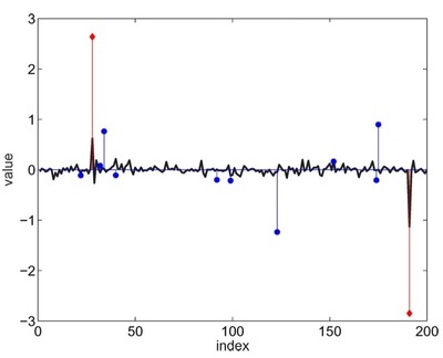
As mentioned in the introduction, communication with compressed data is only possible when both sender and receiver of data understand the decoding method [26, 27, 28]. In data compression, by utilizing the method under our study, we primarily multiply the matrix (features will be explained further) by a sparse vector which we intend to compress in order to obtain a novel vector . If we assume , the new and obtained signal has a shorter length compared to the main signal. The above trend is illustrated in figure 1.

The operation of the main data retrieving is essential in data compression. If we can retrieve signal from compressed signal , a systematic method of data compression and retrieving is obtained for the data. As it will be explained further, without any condition over matrix and vector , retrieving the main data is not possible. In the following sections, we will discuss and describe this issue more precisely.
2.2 Sparse Signals Definition
Sparse signal is commonly referred to a signal having numerous zero elements; in other words, its nonzero elements have a smooth and small signal. The physiology data studied in [29] is a good example of sparse signals that are critical for transmission over communication channels. Failure in transmission of physiology sparse data can incur critical costs to patients [29]. In this work, we use the data set provided by Hosseini et al. [29] to test various deterministic compressed sensing methods on data provided by them, which can be used as a supplementary method to their route selesction method for speeding data transmission in ambulatory transportations. Next, we define sparse signal precisely. Matrix in the base of is called -Sparse if the relation is as given below [30, 31, 32, 33]:
| (1) |
In fact, note that should not have zero determinant in order to be used as a base operator [34].
2.3 Definition of Matrix Coherence
In this section, we merely define matrix coherence terminology and point out its usage in the following subsections. To calculate matrix coherence , it is necessary to obtain the maximum coherence between each two various columns. The coherence of two vectors is also defined as the absolute value of the total arrays of two similar vectors multiplied by each other [39, 40, 41, 42]. We primarily calculate the two inner vectors by multiplying them and then derive its absolute value. If we perform this task for each two separate columns of matrix and find their maximum, matrix coherence is obtained [43, 44, 45, 46].
2.4 Restricted Isometry Property (RIP)
In this section, we also define another concept which is used further. Matrix adhere to RIP from order having a constant value if we have -Sparse for all vectors [34, 47, 48, 49, 50]:
| (2) |
2.5 Features of Matrix compressor
It is worth mentioning that there are two major problems in data compression. First, suitable selection of for maximizing compression of sparse data, and the next problem is reconstructing the main data from compressed signal . Considering the general illustration of operation of compression in figure 1, assume the sparse signal and matrix are available and we intend to reconstruct the main signal , a set of equations having unknown , ought to be solved. As mentioned previously, to have an acceptable compression, there ought to be . However, in this case, the number of unknown is greater than the number of equations which in general, signal reconstructing will be impossible without setting any conditions over the problem. Therefore, we ought to set a condition for matrix and sparse signal to create the possibility to reconstruct the data. With respect to the presented definition, if the signal which is intended to be compressed is sparse order , and if matrix adhere to RIP of order having suitable constant as explained in previous section, it is possible to reconstruct signal -Sparse from noise samples obtaining great results [34].
In addition, it can be shown that it is essential for matrix coherence to limit the signal sparse order to a certain limit (which the coherence depends on it). To generate this type of matrix columns, finite fields are used [51, 52, 53, 54]. In finite field mathematics, there is a field which is comprised of many finite elements. These finite fields are divided with respect to their size. For every measure of the field , a finite field is precisely definable. Note that, is the primary number and as a natural number. The finite fields are broadly applicable in many areas such as mathematics and computer science [24]. The MATLAB code written to produce deterministic matrix is as follows. We used finite fields to produce matrix columns in such a way that fulfills the necessary conditions of output matrix and have low coherence and adhere to RIP from order of by suitable constant .
3 Stochastic and Deterministic Compression of Data
In previous chapter, we became familiar with necessary principle concepts. In this chapter, two general methods are presented to produce matrix . Our focus is on deterministic method. Since the stochastic method has extensive applications, we briefly explain it as well and point out some of its deficiencies.
3.1 Production of Stochastic Matrix
As it was stated in chapter 2, matrix supposed to be valid in a condition with respect to the degree of the sparse signal . Traditionally, matrix was generated stochastically [55, 56, 57, 58, 59]. In fact, every matrix element used to be obtained by a Gaussian stochastic process. By using this method, a negligible value of matrix coherence is highly probable. However, there is no guarantee for the mentioned matrix to adhere to RIP by the order of with a suitable constant , and also have low coherence as well. Therefore, lack of certainty is observed in this method [25, 24]. Furthermore, as stated in the introduction, a communication is possible by time compressed data only if both sender and receiver of data are aware of the details of compression and its method. During this process, it is necessary for both sender and receiver to know matrix to reconstruct the data accurately [60, 61, 62]. Since the sender generates a stochastic matrix during data compression, the receiver has no information about matrix and the sender supposed to transmit matrix along with the compressed data to provide the possibility of reconstructing the main data. In every case mentioned above, the broad band or more memory is used to store , which is not desirable [63, 64, 65]. However, in the proposed method of generating the deterministic matrix, before data compression, matrix is determined for a pair of sender and receiver and there is no need to send or store matrix . Note that the generation of the deterministic matrix can be made fast by utilizing parallel processing of data and using sophisticated MapReduce algorithms, e.g [66, 67, 68, 69, 70, 71, 72, 73].
3.2 Generating deterministic matrix
As explained, by the method of generating deterministic matrix , finite fields are used to generate matrix columns [63, 64, 74, 75, 76]. Note that not only the matrix coherence is smaller than the desired value but also Matrix adhere to RIP from the order with suitable constant as well. It is noteworthy that the matrix elements are no longer stochastic and are generated as systematic matrix thoroughly. At this point, the goal is not to explain how the matrix is generated and for further information, see the article in the reference section [34, 77]. The main goal is to improve the MATLAB code which builds the matrix and to increase the code speed as well as matrix production. The old method of matrix production takes a lot of time overhead in order to produce a large size of data. However, by the new method which will be introduced, this timing is reduced.
First, it is necessary to discuss about deterministic matrix . This matrix has an interesting feature as an assisting agent; if it is complete with respect to size, every matrix column is selected and shifted as circular and then a new circular and shifted vector can be found in one of the columns (circular shift of a vector means that the last vector element is taken and the remaining vector arrays are shifted toward bottom and the last old array is placed in the location of the first vector array). During matrix production by using finite fields, these shifted circular columns are not next to each other. They are usually distributed irregularly along the matrix. Furthermore, we will explain that if shifted circular columns are placed next to each other, we begin from the first matrix column and shift it circularly by a unit value. The outcome vector is in the second matrix column. Now if the second column is shifted circularly by a unit value, the next column which is the third column is generated. We continue this task until no new column is being generated. Therefore, the calculation volume is greatly reduced. Our desired goal is to create similar conditions for the remaining matrix columns. This means that if we select a desired matrix column and shift it circularly, it is precisely in the next column. In this case, the matrix is divided into blocks in which each block would be the shifted circular block of a vector. The general view of ordered and desired matrix is illustrated in figure 3.

In this state, by using the properties of Fourier transfer, the calculation volume in reconstructing will be from order. However, if matrix is not ordered as blocks as explained, the calculation volume in reconstructing will be from order. The reason for having calculation volume reduction is that it is necessary to multiply compressed data by transposes of matrix in the process of reconstructing compressed data. In the case that we intend to carry on this multiplication ordinarily, the calculation volume is from order. So when the matrix is separated in blocks as mentioned, we can remarkably reduce the calculation volume by using the properties of Fourier transform. Instead of multiplying every single column of matrix by , we obtain Fourier transform from the first column of every block and then multiply it by Fourier transform of signal . The next step would be obtaining the opposite of Fourier transform from the result. As a result, the calculation volume is remarkably reduced. To obtain the Fourier transform, it is better to use the FFT command [78, 79, 80, 81, 82, 83] instead of DFT command and for the opposite of Fourier transform, we utilized the IFFT command.
It came to our attention that sorting the matrix as mentioned, reduces the calculation volume remarkably. Therefore, we presently search for a method to sort the matrix quickly which would have a short execution time. In this work two methods are introduced. The first sorting method takes a great deal of time. The second sorting method is very fast and increases the speed of software considerably by utilizing Fourier transform.
3.2.1 The first method of sorting matrix
As stated earlier, it is assumed that by using finite fields, the entire matrix is available and we only intend to sort it into our desirable form. If matrix is complete, the circular shift of the result of every column of matrix can be found in one of its columns. However, if the matrix is not complete, there is possibility that all the results circular shift is not found in the matrix. Therefore, in the first method, the method starts from the first column of matrix and shift it circularly by a unit value, then it continues to the second column. Then the matrix should be searched for this column and if there is such column, it should be replaced. Moreover, if the mentioned column was not found, the first column is shifted twice circularly and the search process has to be done again and if the desired column was found, then place it in the third column of the matrix and delete it from the main matrix. Continue this task until the entire circular shift of the results of the first column are checked. Furthermore, following the same task for other columns until the entire matrix columns are sorted in their related blocks shows that a specific column and circular shift of results are orderly placed next to each other. However, this matrix sorting method is time consuming and has high execution timing. As it will be explained, by the method presented, the execution timing to sort the matrix is highly reduced. Comparing the execution timing of both methods are presented in one graph.
3.2.2 The second method of sorting matrix
As mentioned, we intend to sort matrix in such a way that it is formed by blocks. Moreover, each one of circular shift of the result of vector belongs to one block. If we observe these blocks from frequency point of view, every block column has a common feature. We know that the measure of (abs) of Fourier transform vectors which are circular shift of the result and they are equal to one another. This means that identical vectors can be obtained by performing Fourier transform from the entire columns of the matrix , and each one of the Fourier transform results can be measured by using abs command. Therefore, we can use this final vector as the characteristic of each matrix block. In the next step, we intend to generate a matrix having a big data which its matrix coherence is lower than its data and adhere to RIP from order with suitable constant . They are sorted as blocks which are circularly shifted of separate resulted vectors.
In this method, it is not necessary to generate the entire matrix at the beginning. We primarily generate a column of the matrix (This task is done by finite fields to find the precise method, see the references) and place it in the first column of the matrix . As we know, the first column entire circular shifts can be part of the matrix. Therefore, instead of receiving help from finite fields and its related software to generate the second column matrix again, we shift the first column by a unit value manually and place it in the second column. Subsequently, we shift the second column by a unit value circularly and place it in the third column and continue this process until the first column has been achieved. In this stage, if the necessary length for matrix was not generated, we generate a new column and place it next to other columns and shift it circularly as much as possible, and then set it next to one another. However, the issue is that there is a probability for the new column to be repetitive. In fact, when we generate the previous columns and shift them, it is possible for the new generated column to be among the columns that were circularly shifted. So we should check this problem that whether or not there is a new generated column among the entire generated columns alongside with circularly shifted ones. If we intend to check a new generated column one at a time, it is very time consuming. Especially considering the scenario in which the matrix size becomes large. Hence, the characteristic of every block has been used. As stated, the size of Fourier method of the entire columns belonging to a block are equal to one another. Therefore, after every production of a column it is recommended to assure that the column is not repetitive and shifted and would be placed next to each other. One vector is stored as representative of the mentioned block, which has the same norm as Fourier transform of one of the column of that block. Next, if we produce a new column, we perform Fourier transform on it and then its size would be calculated. The produced vector is compared with the characteristics of previous blocks produced (the characteristics of each block means the size of Fourier transform of one of the columns of that block). If the size of Fourier transform of the new column is equal to the characteristic of one of the previous blocks, we realize that the new and produced column is repetitive and we would have to generate a new column. However, if it is not equal to none of the blocks characteristics, we conclude that the new column produced is not repetitive and there is a possibility to add this column alongside with its circular shift to the matrix. By this method, the speed of production of matrix is remarkably increased. In real time applications, one of the vital issues is to speed up the processing and data compression. As shown in the graph below, the new method presented generates the desirable matrix at a very fast rate. In the graph below, the time it takes to produce the matrix based on various lengths is presented for both methods. It should be mentioned that in order to have the possibility to compare both methods appropriately, the matrix the same coherence should be considered for both methods. In figure 4, the time needed to produce the matrix by the first method is colored by blue and the time needed to produce the matrix by the new method presented is colored by red.

As it is observed, the time needed to generate the matrix by the new method is greatly smaller than the old method. Moreover, as the Matrix length grows the new method is showing better efficiency.
4 Comparing Various Methods of Data Reconstructing
To reconstruct the compressed data, there are various methods. To compare the efficiency of these methods, we have various criteria. Several common methods of data reconstructing were mentioned in [84, 85]. Some of these methods are as follows to name but a few. OMP [86], CoSamp [87, 88, 89, 90, 91, 92], Yall1 [93], IHT [94], IMAT, OMP_enhanced, AMP [95] and CoSamp_enhanced. The last two methods are applicable when the matrix is generated deterministically and its columns are sorted as shown in figure 3. It is noteworthy that the last two methods have higher speed compared to other methods as they are used to compress and reconstruct data by deterministic matrix.
In the next section, we discuss the four criteria to compare the efficiency of aforementioned methods.
4.1 Phase Transition
Assume to be a constant number for the length of compressor matrix . In this case, as stated previously, m shows the number of samples taken from vector , which would be a vector from -sparse order. It is evident that the larger number is and as a result, more samples are taken from vector , the data reconstructing is done by a higher ratio of signal power to noise power. Sometimes we should make sacrifices in data compression with a higher ratio. Assuming no noise is collected by a compressed signal, it is expected that the ratio of signal power to noise to be infinitive. However, these reconstructing methods use algorithms which tend toward numerous or even infinitive repetitive answers. Consequently, there is no possibility to practically reconstruct data precisely [96, 97]. On the other hand, MATLAB software has limited capability to store numbers that have many decimals, which is a factor to avoid obtaining the ratio of signal to high noises for reconstructed signals. Moreover, the lesser is the degree of sparseness of vector the easier it would be to compress the data in by a higher ratio which means by choosing a smaller for matrix we will avoid losing the main signal data.
By the aforementioned introduction, we define the phase transition graph. Assume n to be constant number and the value of changes from to . Then, we change the degree of sparseness of signal from to . For every value of and the sparse vectors from order by numerous repetition are generated and we compress them by stochastic matrix . Subsequently, by using one of the reconstructing methods, the signal would be reconstructed. Finally, with respect to the main signal being available, we obtain the ratio of signal power to noise power for reconstructed signal. If signal to noise is more than a certain value (threshold), we consider the reconstructing to be accurate. Otherwise, we consider the reconstructing to be inaccurate. We divide the number of accurate reconstructing over the entire number of repetitions to figure out the reconstructing percentage. For all valid m and k values, the percentage of accurate data reconstructing for determined m and k in a 3D graph is presented and entered. The horizontal axis ratio of m/n is less than 1, its vertical axis ratio is also smaller than 1, and its height axis shows the accurate reconstructing for specific m and k. Furthermore, we present a precise definition of phase transition by giving two examples from phase transition graphs.
In figure 5, a phase transition graph is presented for a matrix having a length . AMP compression method has been used. The number of repetition for the purpose of obtaining the accurate reconstructing percentage is 200 times for every m and k. Moreover, the value of threshold to evaluate the accuracy of reconstructing is 50 db. In order to use AMP reconstructing method, the maximum considered input error is chosen to be 1e-8 and 200, to obtain an answer as well as the maximum number of repetition (in every reconstructing trial).

As it can be observed in figure 5, for every specific , the AMP method executes the data reconstructing for signals by a sparse order having 100% reconstructing. From a higher sparse order, the reconstructing order is reduced. If the number of repetition is chosen to be a large number to obtain reconstructing percentage, for every m, the reconstructing is done until a sparse order and accurate reconstructing percentage is 100%. Furthermore, the reconstructing percentage suddenly becomes zero after that reconstructing order. The line that separates these two zones of 100% reconstructing and zero percentage is called phase transition. This line is shown in figure 5.
In figure 6, the phase transition graph is presented for CoSamp reconstructing method. In this example, to find an answer for the main signal by CoSamp method, the matrix length is equal to 49, the number of repetition for obtaining the accurate reconstructing percentage is equal to 200. The value of threshold to evaluate the accuracy of reconstructing data is 50 db and the maximum error is considered to be 1e-8.

As it is observed, it seems that data reconstructing by CoSamp method is done for area greater than and . In the next section, we discuss the other criterion to compare various reconstructing methods.
4.2 The ratio of signal to output noise to signal to input noise (SNRout-SNRin)
In this section, we intend to draw one graph to compare the graphs for signal power. The ratio output noise to the input noise of signal power will be compared for various reconstructing methods. To draw this graph, we consider the dimensions of matrix and also the order of sparseness of vector to be constant. In other words, numerical values of m, n, and k are constant. Assume that signal to input noise is a conventional number. In order to measure signal to output noise, it is necessary to generate sparse signal from K order for numerous repetitions. The multiplication resultant of is equal to which is calculated. We add this result with Guassian noise . To obtain the signal to input noise, it is necessary to calculate a coefficient before adding noise to compressed signal . The coefficient is obtained by the following equations after calculation of power of and the power of noise.
| (3) |
Therefore, the signal under reconstructing process is calculated by the following equation by the considered signal to noise.
| (4) |
By using the reconstructing methods, the noise signal will be reconstructed. In this case, signal is obtained. The reconstructed signal has noise and since we have signal , we can obtain the signal to output noise. As it is stated earlier, the operation is would be repeated to obtain signal to output noise. In this case, by calculating the average of signal to output noises, a good average of the ratio of signal to output noise to signal to input noise can obtained. If continue this trend for various signal to input, we can draw the graph of ratio of signal to output noise to signal input noise for one or several reconstructing methods.
As a sample, the graph of ratio of signal to output noise to signal input noise is presented in figure 7 for two reconstructing methods of Yall1 and IHT. In the simulation, and are selected to be equal to 49,25 and 10 respectively. In addition, the signal to input noise is considered to be between 40 db and 100 db. The signal variance and noise are generated stochastically and is equal to one. The number of repetition for calculating the ratio of signal to output noise to signal to input noise constant is 1000 times. The number of signal to input noise is chosen to be 30 by having an equal distance from each other within the range of 40 db and 100 db. The maximum error for finding the main signal answer in Yall1 method is 1e-7 with the maximum number of repetition 1000 (for obtaining an answer in every reconstructing trial).

As it is observed, by the input data given by two methods of IHT and Yall1, the signal to output noise is greater for IHT method compared to Yall1 method. Therefore, IHT method is more efficient compared to Yall1 method. In fact, the execution time of these two methods are not compared. It is possible that the reconstructing timing is higher in IHT method compared to Yall1 method by the data input given to both methods. A more precise comparison can be done when the execution timing between these two methods are compared as well. If we consider input 1e-7 as the error of Yall1 and 1000 repetition as the input for method IHT, then the IHT method has higher efficiency.
In figure 8, the graph of ratio of signal to output noise to signal to input noise is presented for two methods of OMP_enhanced and COSamp_enhanced. To use these two methods, the matrix is generated deterministically, because the reconstructing algorithm in OMP_enhanced and CoSamp_enhanced are designed and generated deterministically for matrices . In simulation, and are chosen to be 125 and 8. Since matrix is generated deterministically, m is determined for matrix with respect to predetermined algorithm which generates . The numerical value of m is not available for the user in this case. To produce matrix stochastically, besides , the numerical value of mu which is the maximum coherence between columns of matrix should be determined. In addition, input which should be the first number representing the elements of which are formed by how many separate components needs be determined as well. For example, if chooses the numerical value of 2, matrix elements are formed from 1 and -1 or a coefficient of 1 and -1. Moreover, if chooses the numerical value of 3, the matrix elements are formed by various elements which the numerical value of 3 is a distinct. In this simulation, the maximum coherence between columns of matrix is equal to 1 and is designated to be 5. In this case, the number of matrix rows is obtained to be 24. The signal to input noise interval is assigned to be 40 db and 100 db. The signal variance and noise are generated stochastically and is equal to 1 and the number of repetition for measuring signal to output noise for signal to constant input noise is 1000 times. The number of signal to input noise is equal to 30 which is chosen at an equal distance between 50 db and 100 db. The maximum error for finding the main signal answer is equal to 1e-8 in CoSamp_enhance method. Matrix is generated deterministically.

As it is observed in figure 8, the signal to output noise for both methods of OMP_enhanced and CoSamp_enhanced does not differ considerably. In fact, it is observed that by using OMP_enhanced method, signal to noise is a little more than when we use CoSamp_enhanced method. However, this difference is not remarkable. Perhaps, it is too early to conclude that these two methods efficiencies do not differ greatly in compressed data reconstructing. We draw the graph of execution timing for every reconstructing method. The execution time that is needed to draw the above graph by using OMP_enhanced, and CoSamp_enhanced methods are 98 and 791 seconds. It is crystal clear that the signal to output noise is higher for OMP_enhanced method compared to CoSamp_enhanced method and also its execution time is greatly less than CoSamp_enhanced method.
4.3 The ratio of signal to noise in order of sparse signal
The third criteria presented to compare the various reconstructing methods is the graph of ratio of signal to output noise to the order of sparseness of signal . To draw this graph, we consider the matrix dimensions to be constant. First, assume that the order of sparseness of signal is constant. signals by the order of sparseness are generated. First, we compress them by matrix , and then, as explained in previous section, (the equations 3 and 4), we add a noise ratio to a specific signal to noise taken from a user to the signal in order to obtain signal . Eventually, the signal would be reconstructed by one of the reconstructing methods. Moreover, since the main signal is available, we can find signal to output noise. Estimation of the signal to output noise would be possible by calculating the average of the signal to output noises obtained in repetitions. If we change the order of signal sparseness from 1 to the maximum order of sparseness (which a user determines and intends to observe it on the graph), the graph of ratio of signal to output noise to sparseness order could be generated. We intend to draw the ratio of signal to noise to the order of sparseness for three methods. These three methods would be AMP, IHT and IMAT and then we deciphered the result. In order to do so, the dimensions of matrix are considered to be as n=49, m=25, and the maximum sparseness order of signal is equal to 20. In addition, the number of repetitions to obtain the signal to output noise is assigned to be equal to 500. The signal to input noise is equal to 15 db, and signal variance which is generated stochastically, is equal to 1. Each one of the reconstructing methods have specific and separate inputs. In AMP reconstructing method, the maximum repetition to obtain an answer is equal to 200 and the maximum error to obtain an answer is assigned to be 1e-8. Regarding IHT reconstructing method, the maximum repetition to obtain an answer is designated to be 1000. In IMAT method, three inputs should be determined by the names of TO, iteration and alfa. The iteration input clearly shows the number of algorithm repetition which is equal to 10,000 in the simulation. However, the other two inputs of and are determined with respect to input signal and its features. In the case which signals are generated stochastically by variance 1, these parameters are chosen to be 7.5 and 0.333 For the numerical values mentioned above, as the input parameters, the ratio of signal to output noise to the order of sparseness of signal is presented in figure 9. (Matrices are generated stochastically).

With respect to figure 9, signal to output noise for the order of sparseness 1 is higher in the IHT reconstructing method in comparison to the other mentioned methods. Afterwards, IMAT and AMP methods respectively have more signal to output noises. In the interval between 2 and 6 for the sparse order, IHT, AMP and IMAT methods respectively allocate the most signal to noises to themselves. For the interval between 7 and 9 for the sparse order, the reconstructing methods AMP, IHT and IMAT respectively have the most signal to output noises. Finally, in high sparse orders between 10 and 20, AMP, IMAT and IHT respectively have more efficiency to obtain the signal to output noise. In the next step, we examine OMP_enhance and CoSamp_enhanced methods. In this case, the numerical values of n, p and the maximum coherence of matrix columns are assigned to be 125, 5, and 1. In this case, the numerical value of m for deterministic matrix is equal to 24. The maximum order of sparseness of signal is chosen to be 20. The signal to input noise is selected to be 15 db and the number of repetition to obtain the signal to output noise is chosen to be 500. Moreover, the signal variance stochastically generated is chosen to be equal to 1. In addition, the specialized input of CoSamp_enhanced method is assigned to be 1e-8 as well. In this case, the ratio of signal to noise to the order of sparseness of signal is illustrated in figure 9 for the both aforementioned methods. As it is observed in figure 10, in the small orders of both methods of OMP_enhanced and CoSamp_enhanced, they do not differ considerably from signal to noise point of view. However, by enlarging the order of sparseness, the OMP_enhanced reconstructing method exhibits better efficiency. If we pay attention to the CoSamp_enhanced reconstructing method, sudden and intense drops occur in the signal to output noise in sparse order 9.

In the next section, we present the last criteria to compare various reconstructing methods.
4.4 The ratio of percentage of reconstructing to the order of signal sparseness
The last criteria which we intend to examine is the ratio of reconstructing percentage to the order of sparseness of signal . To draw this graph, the matrix dimensions ( and ) are considered to be constant. We generate the signals repetition from order numerously. Be careful that we presently consider the order of sparseness to be constant. We compress the signals by multiplying it by matrix . In this section, without adding compressed signal to noise, we reconstruct by one of the reconstructing methods. Since the main signal is available, we can obtain the signal to output noise because no noise is added to the compressed signal . We compare the signal to output noise with the numerical value of a threshold that the user has selected. If the signal to output noise is more than or equal to threshold, the reconstructing is precise and accurate. Otherwise, we consider the reconstructing to be inaccurate. One can obtain the percentage of reconstructing by calculating the ratio of number of accurate reconstructing to the number of all repetitions for the specific order of sparseness. If we change the order of sparseness of signal which is determined by a user, and also if we carry on the above procedures to obtain the reconstructing percentage for every order of sparseness, we can draw the graph of accurate reconstructing percentage based on the order of sparseness. Furthermore, we intend to draw and compare the graph of reconstructing percentage based on the order of sparseness for the reconstructing methods of AMP, OMP and CoSamp. For this task, the matrix dimensions are chosen as n=49 and n=25. The maximum order of signal sparseness is equal to 20 and signal variance is assigned as 1 which is generated stochastically. In addition, the number of repetition is taken as 500 to obtain the reconstructing percentage for specific sparseness order. The special input of AMP method which is the maximum number of repetition as well as the maximum reconstructing algorithm error are chosen as 200 and 1e-8 respectively. Regarding reconstructing methods of OMP and CoSamp, the maximum reconstructing error is only defined as input which is equal to 1e-8. For all three reconstructing methods, the numerical value of threshold of signal to noise is assigned to be 50. The graph of the ratio of accurate reconstructing percentage to the order of sparseness of signal for input data given above is illustrated in figure 11.
By carefully examining the figure 11, it is observed that till the order of 4 of sparseness signal, no considerable difference is seen. As the order grows higher than 4, the reconstructing method of OMP has higher reconstructing percentage compared to the two other methods. From sparseness order 6 to 10. The CoSamp method yields better answer. However, between 11 to 14 the sparseness order changes and the reconstructing method of AMP functions better than CoSamp method. In fact, the reconstructing percentage is low for both methods. From the sparseness order higher than 15, none of the methods are able to reconstruct the signal . (Matrix are generated stochastically.)

In the next step, we draw and compare the graph of ratio of accurate reconstructing percentage to the order of sparseness of signal for two methods of OMP-enhanced and CoSamp_enhanced. With respect to the fact that we should use deterministic matrices for both of these reconstructing methods, we allocate the numerical values of n, p and the maximum coherence of matrix as 125, 5 and 1 respectively. After executing the algorithm to generate deterministic matrix, m is obtained as 24. The maximum order of sparseness of signal is chosen to be 20. The number of repetition to obtain the signal to output noise is chosen as 500. Moreover, signal variance is generated stochastically which is chosen to be equal to 1. Finally, the maximum error for reconstructing method of CoSamp is taken as 1e-8 (The OMP method has no need to have other input such as the number of algorithm repetition or the maximum reconstructing error). In figure 12, the graph of ratio of reconstructing percentage to the order of sparseness of signal for the above inputs are illustrated. (Matrix QM8N is generated stochastically)

It is crystal clear from figure 4-8 that the accurate reconstructing percentage for OMP_enhanced is considerably better than Cosamp_enhanced method. It is worth mentioning that in reconstructing method Cosamp_enhanced, the reconstructing percentage for orders of sparseness higher than 9 intensely is dropped. This behavior was observed in drawing the graph of ratio of signal to output noise to the order of sparseness as well. As it was stated in previous section, not only the reconstructing method of OMP-enhanced functions better in reconstructing the compressed signal, but also the execution time is much better. Execution time of drawing the graph of ratio of reconstructing percentage to the order of sparseness for reconstructing method of OMP_enhanced is nearly 62 seconds and this number for Cosamp_enhancec method is equal to 492 seconds.
5 The GUI Guide to Draw the Aforementioned Graphs in Chapter 4
The ultimate goal of this project is to use the Graphical User Interface in MATLAB environment to draw the graphs discussed in chapter 4. The main goal is to compare these reconstructing methods easier from different aspects. Therefore, in this project, to facilitate the usage of MATLAB files, a MATLAB environment in realm of GUI MATLAB is provided and shown in figure 13 [98].

In the left menu and above GUI designed, the desirable graph among the graphs presented in chapter 4 could be selected. After selecting the desirable graph, various reconstructing methods are exhibited which can be selected. By choosing the reconstructing method from the first column, the matrix can be generated stochastically or deterministically. However, by selecting reconstructing methods in the second column, the matrix has to be updated. In the bottom and left side of the GUI, there are a series of common inputs which are all identical for all the reconstructing methods. However, by choosing any of reconstructing methods, a window would be open at the right side of the screen which receives the special inputs of reconstructing method. By selecting all the reconstructing methods in the first column, the GUI page is formed as figure 14.

Although the majority of inputs were explained along the report, as a comprehensive explanation and easier reference, we explain the entire inputs. The first input named as n_random shows the number of columns of matrix (for both stochastic and deterministic matrices). The m_random input shows the number of columns of matrix in the case in which matrix is generated stochastically. The var_signal input and var_noise input show the signal variance and the signal to noise respectively. The input shows the order of sparseness of signals , SNRin_min, and SNR_max. The mu shows the maximum coherence between matrix columns for the scenario in which it is generated deterministically. The number p is also the first number showing that the matrix elements can be assigned to several separate numerical values. If is equal to 2, the matrix elements are formed from 1 to -1 or from one of their coefficients. Moreover, if P is equal to 3, the matrix elements are formed by three mixed and separate numbers. The plotting precision input is applicable to draw the graph of ratio of signal to output noise to the signal to input noise. The signal to output noise is calculated for several various numerical values from the signal to input noise. To draw the graph of ratio of the signal to output noise to the order of sparseness of signal , we have to determine the size of signal to input noise. This number is determined based on db in SNR-in input. To draw the two graphs of ratio of the signal to output noise to the order of sparseness and the ratio of reconstructing percentage to the order of sparseness, the order of sparseness of signal changes from 1 to its maximum numerical value. The aforementioned maximum numerical value is determined in the input called Sparsity_max. The iteration input shows that how many iterations would occur in order to compute the signal to output noise or the reconstructing percentage. Finally, there is a button called Phi_user as input which provides the possibility to upload desirable matrix and also to draw the graph for the matrix. After choosing any of the reconstructing methods, a window is exhibited at the right side of the screen which shows the reconstructing method. For reconstructing methods of AMP, IHT and IMAT, we have the inputs of AMP-nsweep, IHT-iteration and IMAR-iteration which exhibit the maximum repetition of AMP, IHT and IMAT algorithms. In addition, the reconstructing methods of AMP, OMP, Yall1 and CoSamp_enhanced have the inputs of AMP-tolerance, OMP_tolerance, CoSamp_tplerance, Yall1_tolerance and CoSamp_enhanced_tolerance which exhibit the maximum error of the reconstructed signals. The reconstructing method of OMP_enhanced has no special input. However, the IMAT method has two more inputs called IMAT_T0 and IMAT_Alfa. IMAT_T0 and IMAT_Alfa differ for various signals of with different features. Their numerical values of these inputs have to be adjusted manually. If we generate the signals stochastically by variance 1, these two inputs are selected to be equal to 7.5 and 0.333 respectively. By choosing the specific graph from the above menu and selecting the reconstructing methods with specific inputs, the results would be displayed after choosing the “Process” bottom at the right side and bottom of the screen.
6 Conclusion and Future Work
In this work, we studied different deterministic compressed sensing approaches including AMP, IHT, IMAT, YALL1, CoSamp, and compared them against each other and developed a GUI interface for the user to be able to compare these algorithms. Sparse signals have extensive applications in physiological signal processing [99, 100, 101, 29, 102, 103], communication [104], text compression [105], image processing [106, 107, 108], and etc., where the mentioned compressing methods in this email can be used for a better compression. For future work, one can focus on the different applications of sparse signals and apply the deterministic compressed sensing to them.
References
- [1] M. Burrows, D. J. Wheeler, A block-sorting lossless data compression algorithm.
- [2] J. Ziv, A. Lempel, A universal algorithm for sequential data compression, IEEE Transactions on information theory 23 (3) (1977) 337–343.
- [3] I. H. Witten, R. M. Neal, J. G. Cleary, Arithmetic coding for data compression, Communications of the ACM 30 (6) (1987) 520–540.
- [4] W. B. Pennebaker, J. L. Mitchell, JPEG: Still image data compression standard, Springer Science & Business Media, 1992.
- [5] T. C. Bell, J. G. Cleary, I. H. Witten, Text compression, Vol. 348, Prentice Hall Englewood Cliffs, 1990.
- [6] K. Sayood, Introduction to data compression, Elsevier, 2005.
- [7] D. Salomon, Data compression: the complete reference, Springer Science & Business Media, 2004.
- [8] M. Noormohammadpour, C. S. Raghavendra, Datacenter traffic control: Understanding techniques and trade-offs, IEEE Communications Surveys & Tutorials.
- [9] A. Yekkehkhany, Near data scheduling for data centers with multi levels of data locality, (Dissertation, University of Illinois at Urbana-Champaign).
- [10] M. Noormohammadpour, C. S. Raghavendra, S. Rao, Dcroute: Speeding up inter-datacenter traffic allocation while guaranteeing deadlines, in: High Performance Computing (HiPC), 2016 IEEE 23rd International Conference on, IEEE, 2016, pp. 82–90.
- [11] B. Spolsky, Reduced redundancy as a language testing tool.
- [12] R. F. i Cancho, R. V. Solé, The small world of human language, Proceedings of the Royal Society of London B: Biological Sciences 268 (1482) (2001) 2261–2265.
- [13] http://fa.wikipedia.org/wiki/Datacompression.
- [14] C. Berrou, A. Glavieux, P. Thitimajshima, Near shannon limit error-correcting coding and decoding: Turbo-codes. 1, in: Communications, 1993. ICC’93 Geneva. Technical Program, Conference Record, IEEE International Conference on, Vol. 2, IEEE, 1993, pp. 1064–1070.
- [15] L. Bahl, J. Cocke, F. Jelinek, J. Raviv, Optimal decoding of linear codes for minimizing symbol error rate (corresp.), IEEE Transactions on information theory 20 (2) (1974) 284–287.
- [16] S. Hall, Encoding/decoding, Media and cultural studies: Keyworks 2.
- [17] A. Viterbi, Error bounds for convolutional codes and an asymptotically optimum decoding algorithm, IEEE transactions on Information Theory 13 (2) (1967) 260–269.
- [18] P. B. Gough, W. E. Tunmer, Decoding, reading, and reading disability, Remedial and special education 7 (1) (1986) 6–10.
- [19] I. Daubechies, M. Defrise, C. De Mol, An iterative thresholding algorithm for linear inverse problems with a sparsity constraint, Communications on pure and applied mathematics 57 (11) (2004) 1413–1457.
- [20] E. J. Candes, M. B. Wakin, S. P. Boyd, Enhancing sparsity by reweighted ℓ 1 minimization, Journal of Fourier analysis and applications 14 (5-6) (2008) 877–905.
- [21] R. Tibshirani, M. Saunders, S. Rosset, J. Zhu, K. Knight, Sparsity and smoothness via the fused lasso, Journal of the Royal Statistical Society: Series B (Statistical Methodology) 67 (1) (2005) 91–108.
- [22] K. Egiazarian, A. Foi, V. Katkovnik, Compressed sensing image reconstruction via recursive spatially adaptive filtering, in: Image Processing, 2007. ICIP 2007. IEEE International Conference on, Vol. 1, IEEE, 2007, pp. I–549.
- [23] H. Rauhut, K. Schnass, P. Vandergheynst, Compressed sensing and redundant dictionaries, IEEE Transactions on Information Theory 54 (5) (2008) 2210–2219.
- [24] L. Applebaum, S. D. Howard, S. Searle, R. Calderbank, Chirp sensing codes: Deterministic compressed sensing measurements for fast recovery, Applied and Computational Harmonic Analysis 26 (2) (2009) 283–290.
- [25] R. A. DeVore, Deterministic constructions of compressed sensing matrices, Journal of complexity 23 (4-6) (2007) 918–925.
- [26] I. Amiri, J. Ali, Data signal processing via manchester coding-decoding method using chaotic signals generated by panda ring resonator, Chinese Optics Letters 11 (4) (2013) 041901.
- [27] L. Ikelle, et al., Coding and decoding: Seismic data modeling acquisition and processing, in: 2007 SEG Annual Meeting, Society of Exploration Geophysicists, 2007.
- [28] V. Loia, S. Sessa, Fuzzy relation equations for coding/decoding processes of images and videos, Information sciences 171 (1-3) (2005) 145–172.
- [29] M. Hosseini, Y. Jiang, A. Yekkehkhany, R. R. Berlin, L. Sha, A mobile geo-communication dataset for physiology-aware dash in rural ambulance transport, in: Proceedings of the 8th ACM on Multimedia Systems Conference, ACM, 2017, pp. 158–163.
- [30] R. G. Baraniuk, Compressive sensing [lecture notes], IEEE signal processing magazine 24 (4) (2007) 118–121.
- [31] K. D. Ba, P. Indyk, E. Price, D. P. Woodruff, Lower bounds for sparse recovery, in: Proceedings of the twenty-first annual ACM-SIAM symposium on Discrete Algorithms, SIAM, 2010, pp. 1190–1197.
- [32] H. Shen, J. Z. Huang, Sparse principal component analysis via regularized low rank matrix approximation, Journal of multivariate analysis 99 (6) (2008) 1015–1034.
- [33] T. Zhang, Sparse recovery with orthogonal matching pursuit under rip, IEEE Transactions on Information Theory 57 (9) (2011) 6215–6221.
- [34] http://en.wikipedia.org/wiki/Finite_field.
- [35] P. L. Toint, On sparse and symmetric matrix updating subject to a linear equation, Mathematics of Computation 31 (140) (1977) 954–961.
- [36] A. K. Fletcher, S. Rangan, V. K. Goyal, Necessary and sufficient conditions for sparsity pattern recovery, IEEE Transactions on Information Theory 55 (12) (2009) 5758–5772.
- [37] D. A. Lorenz, Convergence rates and source conditions for tikhonov regularization with sparsity constraints, Journal of Inverse and Ill-Posed Problems 16 (5) (2008) 463–478.
- [38] A. Beck, Y. C. Eldar, Sparsity constrained nonlinear optimization: Optimality conditions and algorithms, SIAM Journal on Optimization 23 (3) (2013) 1480–1509.
- [39] G. Pass, R. Zabih, J. Miller, Comparing images using color coherence vectors, in: Proceedings of the fourth ACM international conference on Multimedia, ACM, 1997, pp. 65–73.
- [40] L. Wen, G. Tan, Image retrieval using spatial multi-color coherence vectors mixing location information, in: Computing, Communication, Control, and Management, 2008. CCCM’08. ISECS International Colloquium on, Vol. 1, IEEE, 2008, pp. 299–302.
- [41] X. Hongli, X. De, G. Yong, Region-based image retrieval using color coherence region vectors, in: Signal Processing, 2004. Proceedings. ICSP’04. 2004 7th International Conference on, Vol. 1, IEEE, 2004, pp. 761–764.
- [42] T. Zhou, J. Cui, G. L. Long, Measure of nonclassical correlation in coherence-vector representation, Physical Review A 84 (6) (2011) 062105.
- [43] P. Drineas, M. Magdon-Ismail, M. W. Mahoney, D. P. Woodruff, Fast approximation of matrix coherence and statistical leverage, Journal of Machine Learning Research 13 (Dec) (2012) 3475–3506.
- [44] A. Talwalkar, A. Rostamizadeh, Matrix coherence and the nystrom method, arXiv preprint arXiv:1408.2044.
- [45] M. Bjørnerud, H. Zhang, Flow mixing, object-matrix coherence, mantle growth and the development of porphyroclast tails, Journal of Structural Geology 17 (9) (1995) 1347–1350.
- [46] M. W. Mahoney, P. Drineas, M. Magdon-Ismail, D. P. Woodruff, Fast approximation of matrix coherence and statistical leverage., in: ICML, 2012.
- [47] E. J. Candes, The restricted isometry property and its implications for compressed sensing, Comptes rendus mathematique 346 (9-10) (2008) 589–592.
- [48] R. Baraniuk, M. Davenport, R. DeVore, M. Wakin, A simple proof of the restricted isometry property for random matrices, Constructive Approximation 28 (3) (2008) 253–263.
- [49] M. A. Davenport, M. B. Wakin, Analysis of orthogonal matching pursuit using the restricted isometry property, IEEE Transactions on Information Theory 56 (9) (2010) 4395–4401.
- [50] F. Krahmer, R. Ward, New and improved johnson–lindenstrauss embeddings via the restricted isometry property, SIAM Journal on Mathematical Analysis 43 (3) (2011) 1269–1281.
- [51] A. J. Menezes, T. Okamoto, S. A. Vanstone, Reducing elliptic curve logarithms to logarithms in a finite field, iEEE Transactions on information Theory 39 (5) (1993) 1639–1646.
- [52] I. S. Reed, G. Solomon, Polynomial codes over certain finite fields, Journal of the society for industrial and applied mathematics 8 (2) (1960) 300–304.
- [53] J. M. Pollard, The fast fourier transform in a finite field, Mathematics of computation 25 (114) (1971) 365–374.
- [54] D. Quillen, On the cohomology and k-theory of the general linear groups over a finite field, Annals of Mathematics (1972) 552–586.
- [55] D. L. Donoho, Compressed sensing, IEEE Transactions on information theory 52 (4) (2006) 1289–1306.
- [56] M. Lustig, D. Donoho, J. M. Pauly, Sparse mri: The application of compressed sensing for rapid mr imaging, Magnetic resonance in medicine 58 (6) (2007) 1182–1195.
- [57] E. J. Candès, M. B. Wakin, An introduction to compressive sampling, IEEE signal processing magazine 25 (2) (2008) 21–30.
- [58] E. J. Candès, et al., Compressive sampling, in: Proceedings of the international congress of mathematicians, Vol. 3, Madrid, Spain, 2006, pp. 1433–1452.
- [59] Z. Tian, G. B. Giannakis, Compressed sensing for wideband cognitive radios, in: Acoustics, Speech and Signal Processing, 2007. ICASSP 2007. IEEE International Conference on, Vol. 4, IEEE, 2007, pp. IV–1357.
- [60] S. Li, F. Gao, G. Ge, S. Zhang, Deterministic construction of compressed sensing matrices via algebraic curves, IEEE Transactions on Information Theory 58 (8) (2012) 5035–5041.
- [61] R. Calderbank, S. Howard, S. Jafarpour, Construction of a large class of deterministic sensing matrices that satisfy a statistical isometry property, IEEE journal of selected topics in signal processing 4 (2) (2010) 358–374.
- [62] S. D. Howard, A. R. Calderbank, S. J. Searle, A fast reconstruction algorithm for deterministic compressive sensing using second order reed-muller codes, in: Information Sciences and Systems, 2008. CISS 2008. 42nd Annual Conference on, IEEE, 2008, pp. 11–15.
- [63] N. Y. Yu, Y. Li, Deterministic construction of fourier-based compressed sensing matrices using an almost difference set, EURASIP Journal on Advances in Signal Processing 2013 (1) (2013) 155.
- [64] K. Li, C. Ling, L. Gan, Deterministic compressed-sensing matrices: Where toeplitz meets golay, in: Acoustics, Speech and Signal Processing (ICASSP), 2011 IEEE International Conference on, IEEE, 2011, pp. 3748–3751.
- [65] M. Bayati, A. Montanari, The dynamics of message passing on dense graphs, with applications to compressed sensing, IEEE Transactions on Information Theory 57 (2) (2011) 764–785.
- [66] J. Dean, S. Ghemawat, Mapreduce: simplified data processing on large clusters, Communications of the ACM 51 (1) (2008) 107–113.
- [67] J. Dean, S. Ghemawat, Mapreduce: a flexible data processing tool, Communications of the ACM 53 (1) (2010) 72–77.
- [68] C.-T. Chu, S. K. Kim, Y.-A. Lin, Y. Yu, G. Bradski, K. Olukotun, A. Y. Ng, Map-reduce for machine learning on multicore, in: Advances in neural information processing systems, 2007, pp. 281–288.
- [69] A. Yekkehkhany, A. Hojjati, M. H. Hajiesmaili, Gb-pandas:: Throughput and heavy-traffic optimality analysis for affinity scheduling, ACM SIGMETRICS Performance Evaluation Review 45 (2) (2018) 2–14.
- [70] M. Zaharia, A. Konwinski, A. D. Joseph, R. H. Katz, I. Stoica, Improving mapreduce performance in heterogeneous environments., in: Osdi, Vol. 8, 2008, p. 7.
- [71] A. Daghighi, M. Kavousi, Scheduling for data centers with multi-level data locality, in: Electrical Engineering (ICEE), 2017 Iranian Conference on, IEEE, 2017, pp. 927–936.
- [72] C. Ranger, R. Raghuraman, A. Penmetsa, G. Bradski, C. Kozyrakis, Evaluating mapreduce for multi-core and multiprocessor systems, in: High Performance Computer Architecture, 2007. HPCA 2007. IEEE 13th International Symposium on, Ieee, 2007, pp. 13–24.
- [73] H.-c. Yang, A. Dasdan, R.-L. Hsiao, D. S. Parker, Map-reduce-merge: simplified relational data processing on large clusters, in: Proceedings of the 2007 ACM SIGMOD international conference on Management of data, ACM, 2007, pp. 1029–1040.
- [74] G. Xu, Z. Xu, Compressed sensing matrices from fourier matrices, IEEE Transactions on Information Theory 61 (1) (2015) 469–478.
- [75] S. Li, G. Ge, Deterministic sensing matrices arising from near orthogonal systems, IEEE Transactions on Information Theory 60 (4) (2014) 2291–2302.
- [76] E. J. Candes, T. Tao, Near-optimal signal recovery from random projections: Universal encoding strategies?, IEEE transactions on information theory 52 (12) (2006) 5406–5425.
- [77] E. J. Candès, J. Romberg, T. Tao, Robust uncertainty principles: Exact signal reconstruction from highly incomplete frequency information, IEEE Transactions on information theory 52 (2) (2006) 489–509.
- [78] P. Welch, The use of fast fourier transform for the estimation of power spectra: a method based on time averaging over short, modified periodograms, IEEE Transactions on audio and electroacoustics 15 (2) (1967) 70–73.
- [79] K. Katoh, K. Misawa, K.-i. Kuma, T. Miyata, Mafft: a novel method for rapid multiple sequence alignment based on fast fourier transform, Nucleic acids research 30 (14) (2002) 3059–3066.
- [80] P. Carr, D. Madan, Option valuation using the fast fourier transform, Journal of computational finance 2 (4) (1999) 61–73.
- [81] C. Van Loan, Computational frameworks for the fast Fourier transform, Vol. 10, Siam, 1992.
- [82] E. O. Brigham, E. O. Brigham, The fast Fourier transform and its applications, Vol. 1, prentice Hall Englewood Cliffs, NJ, 1988.
- [83] W. T. Cochran, J. W. Cooley, D. L. Favin, H. D. Helms, R. A. Kaenel, W. W. Lang, G. C. Maling, D. E. Nelson, C. M. Rader, P. D. Welch, What is the fast fourier transform?, Proceedings of the IEEE 55 (10) (1967) 1664–1674.
- [84] http://www.wikihow.com/Build-a-Simple-Graphical-User-Interface-in-Matlab.
- [85] Y. Zhang, J. Yang, W. Yin, User’s guide for yall1: Your algorithms for l1 optimization, Technique report (2009) 09–17.
- [86] D. L. Donoho, M. Elad, V. N. Temlyakov, Stable recovery of sparse overcomplete representations in the presence of noise, IEEE Transactions on information theory 52 (1) (2006) 6–18.
- [87] D. Needell, J. A. Tropp, Cosamp: Iterative signal recovery from incomplete and inaccurate samples, Applied and computational harmonic analysis 26 (3) (2009) 301–321.
- [88] D. Needell, J. A. Tropp, Cosamp: iterative signal recovery from incomplete and inaccurate samples, Communications of the ACM 53 (12) (2010) 93–100.
- [89] M. A. Davenport, D. Needell, M. B. Wakin, Signal space cosamp for sparse recovery with redundant dictionaries, IEEE Transactions on Information Theory 59 (10) (2013) 6820–6829.
- [90] R. Giryes, M. Elad, Rip-based near-oracle performance guarantees for sp, cosamp, and iht, IEEE Transactions on Signal Processing 60 (3) (2012) 1465–1468.
- [91] R. Giryes, M. Elad, Cosamp and sp for the cosparse analysis model, in: Signal Processing Conference (EUSIPCO), 2012 Proceedings of the 20th European, IEEE, 2012, pp. 964–968.
- [92] S. Becker, Cosamp and omp for sparse recovery, Matlab Central File Exchange 8 (2012) 01–11.
- [93] J. Yang, Y. Zhang, Alternating direction algorithms for ell_1-problems in compressive sensing, SIAM journal on scientific computing 33 (1) (2011) 250–278.
- [94] T. Blumensath, M. E. Davies, Iterative hard thresholding for compressed sensing, Applied and computational harmonic analysis 27 (3) (2009) 265–274.
- [95] D. L. Donoho, A. Maleki, A. Montanari, Message-passing algorithms for compressed sensing, Proceedings of the National Academy of Sciences 106 (45) (2009) 18914–18919.
- [96] Y. Wu, S. Verdú, Optimal phase transitions in compressed sensing, IEEE Transactions on Information Theory 58 (10) (2012) 6241–6263.
- [97] S. Dutta, M. Fahim, F. Haddadpour, H. Jeong, V. Cadambe, P. Grover, On the optimal recovery threshold of coded matrix multiplication, arXiv preprint arXiv:1801.10292.
- [98] http://sparselab.stanford.edu/.
- [99] S. Counts, M. Smith, Where were we: communities for sharing space-time trails, in: Proceedings of the 15th annual ACM international symposium on Advances in geographic information systems, ACM, 2007, p. 10.
- [100] S. Lederer, C. Mueller, C. Timmerer, C. Concolato, J. Le Feuvre, K. Fliegel, Distributed dash dataset, in: Proceedings of the 4th ACM Multimedia Systems Conference, ACM, 2013, pp. 131–135.
- [101] H. Riiser, P. Vigmostad, C. Griwodz, P. Halvorsen, Commute path bandwidth traces from 3g networks: analysis and applications, in: Proceedings of the 4th ACM Multimedia Systems Conference, ACM, 2013, pp. 114–118.
- [102] M. T. Alrefaie, road speed profile: from gps traces to real-time traffic speed, in: Proceedings of the 15th ACM international symposium on Mobile ad hoc networking and computing, ACM, 2014, pp. 407–408.
- [103] M. I. Chehardeh, E. M. Siavashi, A closed-loop controller to improve the stability of cascaded dc/dc converters, arXiv preprint arXiv:1802.07159.
- [104] F. Haddadpour, M. H. Yassaee, S. Beigi, A. Gohari, M. R. Aref, Simulation of a channel with another channel, IEEE Transactions on Information Theory 63 (5) (2017) 2659–2677.
- [105] M. Kavousi, S. Saadatmand, Estimating the rating of reviewers based on the text, arXiv preprint arXiv:1805.08415.
- [106] B. Yao, F. Imani, A. S. Sakpal, E. Reutzel, H. Yang, Multifractal analysis of image profiles for the characterization and detection of defects in additive manufacturing, Journal of Manufacturing Science and Engineering 140 (3) (2018) 031014.
- [107] B. Yao, F. Imani, H. Yang, Markov decision process for image-guided additive manufacturing, IEEE Robotics and Automation Letters.
- [108] M. I. Chehardeh, M. M. Almalki, C. J. Hatziadoniu, Remote feeder transfer between out-of-phase sources using sts, in: Power and Energy Conference at Illinois (PECI), 2016 IEEE, IEEE, 2016, pp. 1–5.