跳到论文正文
W Papers独立论文阅读器 arXiv:1807.01051 论文正文 计算阅读时间 · 0%
引用这篇论文根据当前论文元数据生成,正式投稿前建议核对。


License: arXiv.org perpetual non-exclusive license
arXiv:1807.01051v2 [math.GT] 16 Mar 2020

A construction of pseudo-Anosov braids with small normalized entropies

Susumu Hirose Address: Department of Mathematics, Faculty of Science and Technology, Tokyo University of Science, Noda, Chiba, 278-8510, Japan Email address: hirose_susumu@ma.noda.tus.ac.jp and Eiko Kin Address: Department of Mathematics, Graduate School of Science, Osaka University Toyonaka, Osaka 560-0043, JAPAN Email address: kin@math.sci.osaka-u.ac.jp
Date: March 12, 2020.
Abstract.

Let bb be a pseudo-Anosov braid whose permutation has a fixed point and let MbM_{b} be the mapping torus by the pseudo-Anosov homeomorphism defined on the genus 00 fiber FbF_{b} associated with bb. We prove that there is a 22-dimensional subcone 𝒞0\mathcal{C}_{0} contained in the fibered cone 𝒞\mathcal{C} of FbF_{b} such that the fiber FaF_{a} for each primitive integral class a∈𝒞0a\in\mathcal{C}_{0} has genus 00. We also give a constructive description of the monodromy ϕa:Fa→Fa\phi_{a}:F_{a}\rightarrow F_{a} of the fibration on MbM_{b} over the circle, and consequently provide a construction of many sequences of pseudo-Anosov braids with small normalized entropies. As an application we prove that the smallest entropy among skew-palindromic braids with nn strands is comparable to 1/n1/n, and the smallest entropy among elements of the odd/even spin mapping class groups of genus gg is comparable to 1/g1/g.

Key words and phrases: 
mapping class groups, pseudo-Anosov, dilatation, normalized entropy, fibered 33-manifolds, braid group
2010 Mathematics Subject Classification
57M99, 37E30

1. Introduction

Refer to caption
Figure 1. (1) σi\sigma_{i}. (2) σ1−1​σ2\sigma_{1}^{-1}\sigma_{2} with the permutation 1↦21\mapsto 2, 2↦32\mapsto 3, 3↦13\mapsto 1. (3) σ12​σ2−1\sigma_{1}^{2}\sigma_{2}^{-1} whose permutation has a fixed point.
Refer to caption
Figure 2. b:=σ12​σ2−1b:=\sigma_{1}^{2}\sigma_{2}^{-1}. (1) cl⁡(b)\mathrm{cl}(b). (2) br⁡(b)\mathrm{br}(b). (3) Fb↪MbF_{b}\hookrightarrow M_{b}.

Let Σ=Σg,n\Sigma=\Sigma_{g,n} be an orientable surface of genus gg with nn punctures for n≥0n\geq 0. We set Σg=Σg,0\Sigma_{g}=\Sigma_{g,0}. By mapping class group Mod⁡(Σg,n)\mathrm{Mod}(\Sigma_{g,n}), we mean the group of isotopy classes of orientation preserving self-homeomorphisms on Σg,n\Sigma_{g,n} preserving punctures setwise. By Nielsen-Thurston classification, elements in Mod⁡(Σ)\mathrm{Mod}(\Sigma) are classified into three types: periodic, reducible, pseudo-Anosov [30, 9]. For ϕ∈Mod⁡(Σ)\phi\in\mathrm{Mod}(\Sigma) we choose a representative Φ∈ϕ\Phi\in\phi and consider the mapping torus Mϕ=Σ×ℝ/∼M_{\phi}=\Sigma\times{\mathbb{R}}/\sim, where ∼\sim identifies (x,t+1)(x,t+1) with (Φ⁡(x),t)(\Phi(x),t) for x∈Σx\in\Sigma and t∈ℝt\in{\mathbb{R}}. Then Σ\Sigma is a fiber of a fibration on MϕM_{\phi} over the circle S1S^{1} and ϕ\phi is called the monodromy. A theorem by Thurston [31] asserts that MϕM_{\phi} admits a hyperbolic structure of finite volume if and only if ϕ\phi is pseudo-Anosov.

For a pseudo-Anosov element ϕ∈Mod⁡(Σ)\phi\in\mathrm{Mod}(\Sigma) there is a representative Φ:Σ→Σ\Phi:\Sigma\rightarrow\Sigma of ϕ\phi called a pseudo-Anosov homeomorphism with the following property: Φ\Phi admits a pair of transverse measured foliations (ℱu,μu)(\mathcal{F}^{u},\mu^{u}) and (ℱs,μs)(\mathcal{F}^{s},\mu^{s}) and a constant λ=λ⁡(ϕ)>1\lambda=\lambda(\phi)>1 depending on ϕ\phi such that ℱu\mathcal{F}^{u} and ℱs\mathcal{F}^{s} are invariant under Φ\Phi, and μu\mu^{u} and μs\mu^{s} are uniformly multiplied by λ\lambda and λ−1\lambda^{-1} under Φ\Phi. The constant λ⁡(ϕ)\lambda(\phi) is called the dilatation and ℱu\mathcal{F}^{u} and ℱs\mathcal{F}^{s} are called the unstable and stable foliation. We call the logarithm log⁡(λ⁡(ϕ))\log(\lambda(\phi)) the entropy, and call

Ent⁡(ϕ)=|χ⁡(Σ)|​log⁡(λ⁡(ϕ))\mathrm{Ent}(\phi)=|\chi(\Sigma)|\log(\lambda(\phi))

the normalized entropy of ϕ\phi, where χ⁡(Σ)\chi(\Sigma) is the Euler characteristic of Σ\Sigma. Such normalization of the entropy is suited for the context of 33-manifolds [8, 21].

Penner [27] proved that if ϕ∈Mod⁡(Σg,n)\phi\in\mathrm{Mod}(\Sigma_{g,n}) is pseudo-Anosov, then

(1.1) log⁡212​g−12+4​n≤log⁡(λ⁡(ϕ)).\frac{\log 2}{12g-12+4n}\leq\log(\lambda(\phi)).

See also [21, Corollary 2]. For a fixed surface Σ\Sigma, the set

{log⁡λ⁡(ϕ)|ϕ∈Mod⁡(Σ)​is pseudo-Anosov}\{\log\lambda(\phi)\ |\ \phi\in\mathrm{Mod}(\Sigma)\ \mbox{is pseudo-Anosov}\}

is a closed, discrete subset of ℝ{\mathbb{R}} ([1]). For any subgroup or subset G⊂Mod⁡(Σ)G\subset\mathrm{Mod}(\Sigma) let δ⁡(G)\delta(G) denote the minimum of λ⁡(ϕ)\lambda(\phi) over all pseudo-Anosov elements ϕ∈G\phi\in G. Then δ⁡(G)≥δ⁡(Mod⁡(Σ))\delta(G)\geq\delta(\mathrm{Mod}(\Sigma)). We write f≍hf\asymp h if there is a universal constant P>0P>0 such that 1/P≤f/h≤P1/P\leq f/h\leq P. It is proved by Penner [27] that the minimal entropy among pseudo-Anosov elements in Mod⁡(Σg)\mathrm{Mod}(\Sigma_{g}) on the closed surface of genus gg satisfies

log⁡δ⁡(Mod⁡(Σg))≍1g.\log\delta(\mathrm{Mod}(\Sigma_{g}))\asymp\dfrac{1}{g}.

See also [16, 32, 33] for other sequences of mapping class groups.

For any P>0P>0, consider the set ΨP\Psi_{P} consisting of all pseudo-Anosov homeomorphisms Φ:Σ→Σ\Phi:\Sigma\rightarrow\Sigma defined on any surface Σ\Sigma with the normalized entropy |χ⁡(Σ)|​log⁡λ⁡(Φ)≤P|\chi(\Sigma)|\log\lambda(\Phi)\leq P. This is an infinite set in general (take P>2​log⁡(2+3)P>2\log(2+\sqrt{3}) for example) and is well-understood in the context of hyperbolic fibered 33-manifolds. The universal finiteness theorem by Farb-Leininger-Margalit [8] states that the set of homeomorphism classes of mapping tori of pseudo-Anosov homeomprhisms Φ∘:Σ∘→Σ∘\Phi^{\circ}:\Sigma^{\circ}\rightarrow\Sigma^{\circ} is finite, where Φ∘:Σ∘→Σ∘\Phi^{\circ}:\Sigma^{\circ}\rightarrow\Sigma^{\circ} is the fully punctured pseudo-Anosov homeomprhism obtained from Φ∈ΨP\Phi\in\Psi_{P}. (Clearly λ⁡(Φ∘)=λ⁡(Φ)\lambda(\Phi^{\circ})=\lambda(\Phi).) In other words such Φ∘:Σ∘→Σ∘\Phi^{\circ}:\Sigma^{\circ}\rightarrow\Sigma^{\circ} is a monodromy of a fiber in some fibered cone for a hyperbolic fibered 33-manifold in the finite list determined by PP. Thus 33-manifolds in the finite list govern all pseudo-Anosov elements in ΨP\Psi_{P}. It is natural to ask the dynamics and a constructive description of elements in ΨP\Psi_{P}. There are some results about this question by several authors [4, 15, 20, 22, 33], but it is not completely understood. In this paper we restrict our attention to the pseudo-Anosov elements in ΨP\Psi_{P} defined on the genus 00 surfaces, and provide an approach for a concrete description of those elements.

Let BnB_{n} be the braid group with nn strands. The group BnB_{n} is generated by the braids σ1,⋯,σn−1\sigma_{1},\cdots,\sigma_{n-1} as in Figure 1. Let 𝒮n\mathcal{S}_{n} be the symmetric group, the group of bijections of {1,…,n}\{1,\ldots,n\} to itself. A permutation 𝒫∈𝒮n\mathcal{P}\in\mathcal{S}_{n} has a fixed point if 𝒫⁡(i)=i\mathcal{P}(i)=i for some ii. We have a surjective homomorphism π:Bn→𝒮n\pi:B_{n}\rightarrow\mathcal{S}_{n} which sends each σj\sigma_{j} to the transposition (j,j+1)(j,j+1).

The closure cl⁡(b)\mathrm{cl}(b) of a braid b∈Bnb\in B_{n} is a knot or link in the 33-sphere S3S^{3}. The braided link

br⁡(b)=cl⁡(b)∪A\mathrm{br}(b)=\mathrm{cl}(b)\cup A

is a link in S3S^{3} obtained from cl⁡(b)\mathrm{cl}(b) with its braid axis AA (Figure 2). Let MbM_{b} denote the exterior of br⁡(b)\mathrm{br}(b) which is a 33-manifold with boundary. It is easy to find an (n+1)(n+1)-holed sphere FbF_{b} in MbM_{b} (Figure 2(3)). Clearly FbF_{b} is a fiber of a fibration on Mb→S1M_{b}\rightarrow S^{1} and its monodromy ϕb:Fb→Fb\phi_{b}:F_{b}\rightarrow F_{b} is determined by bb. We call FbF_{b} the FF-surface for bb.

A braid b∈Bnb\in B_{n} is periodic (resp. reducible, pseudo-Anosov) if the associated mapping class fb∈Mod⁡(Σ0,n+1)f_{b}\in\mathrm{Mod}(\Sigma_{0,n+1}) is of the corresponding type (Section 2.3). If bb is pseudo-Anosov, then the dilatation λ⁡(b)\lambda(b) is defined by λ⁡(fb)\lambda(f_{b}) and the normalized entropy Ent⁡(b)\mathrm{Ent}(b) is defined by Ent⁡(fb)\mathrm{Ent}(f_{b}). The following theorem is due to Hironaka-Kin [16, Proposition 3.36] together with the observation by Kin-Takasawa [22, Section 4.1].

Theorem 1.1.

There is a sequence of pseudo-Anosov braids zn∈Bnz_{n}\in B_{n} such that Ent⁡(zn)≠2​log⁡(2+3)\mathrm{Ent}(z_{n})\neq 2\log(2+\sqrt{3}), Mzn≃Mσ12​σ2−1M_{z_{n}}\simeq M_{\sigma_{1}^{2}\sigma_{2}^{-1}} for each n≥3n\geq 3 and Ent⁡(zn)→2​log⁡(2+3)\mathrm{Ent}(z_{n})\to 2\log(2+\sqrt{3}) as n→∞n\to\infty.

Here ≃\simeq means they are homeomorphic to each other. The limit point 2​log⁡(2+3)2\log(2+\sqrt{3}) is equal to Ent⁡(σ12​σ2−1)\mathrm{Ent}(\sigma_{1}^{2}\sigma_{2}^{-1}). By the lower bound (1.1), Theorem 1.1 implies that

log⁡δ⁡(Mod⁡(Σ0,n))≍1n.\log\delta(\mathrm{Mod}(\Sigma_{0,n}))\asymp\dfrac{1}{n}.

In particular, the hyperbolic fibered 33-manifold Mσ12​σ2−1M_{\sigma_{1}^{2}\sigma_{2}^{-1}} admits an infinitely family of genus 00 fibers of fibrations over S1S^{1}.

Let znz_{n} be a pseudo-Anosov braid with dnd_{n} strands. We say that a sequence {zn}\{z_{n}\} has a small normalized entropy if dn≍nd_{n}\asymp n and there is a constant P>0P>0 which does not depend on nn such that Ent⁡(zn)≤P\mathrm{Ent}(z_{n})\leq P. By (1.1) a sequence {zn}\{z_{n}\} having a small normalized entropy means log⁡(λ⁡(zn))≍1/n\log(\lambda(z_{n}))\asymp 1/n. One of the aims in this paper is to give a construction of many sequences of pseudo-Anosov braids with small normalized entropies. The following result generalizes Thereom 1.1.

Theorem A.

Suppose that bb is a pseudo-Anosov braid whose permutation has a fixed point. There is a sequence of pseudo-Anosov braids {zn}\{z_{n}\} with small normalized entropy such that Ent⁡(zn)→Ent⁡(b)\mathrm{Ent}(z_{n})\to\mathrm{Ent}(b) as n→∞n\to\infty and Mzn≃MbM_{z_{n}}\simeq M_{b} for n≥1n\geq 1.

The proof of Theorem A is constructive. In fact one can describe braids znz_{n} explicitly. For a more general result see Theorems 5.1, 5.2. Let 𝒞⊂H2​(Mb,∂Mb)\mathcal{C}\subset H_{2}(M_{b},\partial M_{b}) be the fibered cone containing [Fb][F_{b}]. A theorem by Thurston [29] states that for each primitive integral class a∈𝒞a\in\mathcal{C} there is a connected fiber FaF_{a} with the pseudo-Anosov monodromy ϕa:Fa→Fa\phi_{a}:F_{a}\rightarrow F_{a} of a fibration on the hyperbolic 33-manifold MbM_{b} over S1S^{1}. The following theorem states a structure of 𝒞\mathcal{C}.

Theorem B.

Suppose that bb is a pseudo-Anosov braid whose permutation has a fixed point. Then there are a 22-dimensional subcone 𝒞0⊂𝒞\mathcal{C}_{0}\subset\mathcal{C} and an integer u≥1u\geq 1 with the following properties.

  1. (1)

    The fiber FaF_{a} for each primitive integral class a∈𝒞0a\in\mathcal{C}_{0} has genus 00.

  2. (2)

    The monodromy ϕa:Fa→Fa\phi_{a}:F_{a}\rightarrow F_{a} for each primitive integral class a∈𝒞0a\in\mathcal{C}_{0} is conjugate to

    (ω1ψ)⋯(ωu−1ψ)(ωuψ)ψm−1:Fa→Fa,(\omega_{1}\psi)\cdots(\omega_{u-1}\psi)(\omega_{u}\psi)\psi^{m-1}:F_{a}\rightarrow F_{a},

    where m≥1m\geq 1 depends on the class aa, ψ\psi is periodic and each ωj\omega_{j} is reducible. Moreover there are homeomorphisms ω^j:S0→S0\widehat{\omega}_{j}:S_{0}\rightarrow S_{0} on a surface S0S_{0} for j=1,…,uj=1,\ldots,u determined by bb and an embedding h:S0↪Fah:S_{0}\hookrightarrow F_{a} such that h⁡(S0)h(S_{0}) is the support of each wjw_{j} and

    wj|h⁡(S0)=h∘ω^j∘h−1.w_{j}|_{h(S_{0})}=h\circ\widehat{\omega}_{j}\circ h^{-1}.

Theorem B gives a constructive description of ϕa\phi_{a}. Also it states that each wj:Fa→Faw_{j}:F_{a}\rightarrow F_{a} is reducible supported on a uniformly bounded subsurface h⁡(S0)⊂Fah(S_{0})\subset F_{a}. It turns out from the proof that the type of the periodic homeomorphism ψ:Fa→Fa\psi:F_{a}\rightarrow F_{a} does not depend on a∈C0a\in C_{0} (Remark 3.3), see Figure 3(1). Theorem B reminds us of the symmetry conjecture in [23] by Farb-Leininger-Margalit.

Clearly the permutation of each pure braid has a fixed point. For any pseudo-Anosov braid bb, a suitable power bkb^{k} becomes a pure braid and one can apply Theorems A, B for bkb^{k}.

We have a remark about Theorem A. Theorem 10.2 in [25] by McMullen also tells us the existence of a sequence (Fn,ϕn)(F_{n},\phi_{n}) of fibers and monodromies in 𝒞\mathcal{C} such that Ent⁡(ϕn)→Ent⁡(b)\mathrm{Ent}(\phi_{n})\to\mathrm{Ent}(b) as n→∞n\to\infty and |χ⁡(Fn)|≍n|\chi(F_{n})|\asymp n. However one can not appeal his theorem for the genera of fibers FnF_{n}. Theorem A says that FnF_{n} has genus 00 in fact.

Refer to caption
Figure 3. Dynamics of ψ\psi and ωj\omega_{j} in Theorem B. (1) Periodic ψ:Fa→Fa\psi:F_{a}\rightarrow F_{a}. (2) Reducible ωj:Fa→Fa\omega_{j}:F_{a}\rightarrow F_{a}. Subsurface h⁡(S0)h(S_{0}) is shaded.
Refer to caption
Figure 4. Illustration of braids (1) bb, (2) r​e​v​(b)rev(b), (3) s​k​e​w​(b)skew(b).

As an application we will determine asymptotic behaviors of the minimal dilatations of a subset of BnB_{n} consisting of braids with a symmetry. A braid b∈Bnb\in B_{n} is palindromic if r​e​v​(b)=brev(b)=b, where r​e​v:Bn→Bnrev:B_{n}\rightarrow B_{n} is a map such that if ww is a word of letters σj±1\sigma_{j}^{\pm 1} representing bb, then r​e​v​(b)rev(b) is the braid obtained from bb reversing the order of letters in ww. A braid b∈Bnb\in B_{n} is skew-palindromic if s​k​e​w​(b)=bskew(b)=b, where s​k​e​w​(b)=Δ​r​e​v​(b)​Δ−1skew(b)=\Delta rev(b)\Delta^{-1} and Δ\Delta is a half twist (Section 2.2). See Figure 4. We will prove that dilatations of palindromic braids have the following lower bound.

Theorem C.

If b∈Bnb\in B_{n} is palindromic and pseudo-Anosov for n≥3n\geq 3, then

λ⁡(b)≥2+5.\lambda(b)\geq\sqrt{2+\sqrt{5}}.

In contrast with palindromic braids we have the following result.

Theorem D.

Let P​AnPA_{n} be the set of skew-palindromic elements in BnB_{n}. We have

log⁡δ⁡(P​An)≍1n.\log\delta(PA_{n})\asymp\dfrac{1}{n}.
Refer to caption
Figure 5. (1) ℐ:Σg→Σg\mathcal{I}:\Sigma_{g}\rightarrow\Sigma_{g}. (2) A basis {x1,y1,…,xg,yg}\{x_{1},y_{1},\ldots,x_{g},y_{g}\} of H1​(Σg,ℤ2)H_{1}(\Sigma_{g};\mathbb{Z}_{2}).

The hyperelliptic mapping class group ℋ⁡(Σg)\mathcal{H}(\Sigma_{g}) is the subgroup of Mod⁡(Σg)\mathrm{Mod}(\Sigma_{g}) consisting of elements with representative homeomorphisms that commute with some fixed hyperelliptic involution ℐ:Σg→Σg\mathcal{I}:\Sigma_{g}\rightarrow\Sigma_{g} as in Figure 5(1). It is shown in [16] that log⁡δ⁡(ℋ⁡(Σg))≍1/g\log\delta(\mathcal{H}(\Sigma_{g}))\asymp 1/g. See also [7, 15, 19] for other subgroups of Mod⁡(Σg)\mathrm{Mod}(\Sigma_{g}). As an application we will determine the asymptotic behavior of the minimal dilatations of the odd/even spin mapping class groups of genus gg. To define these subgroups let (⋅,⋅)2(\cdot,\cdot)_{2} be the mod-22 intersection form on H1​(Σg,ℤ2)H_{1}(\Sigma_{g};\mathbb{Z}_{2}). A map 𝔮:H1​(Σg,ℤ2)→ℤ2\mathfrak{q}:H_{1}(\Sigma_{g};\mathbb{Z}_{2})\to\mathbb{Z}_{2} is a quadratic form if 𝔮⁡(v+w)=𝔮⁡(v)+𝔮⁡(w)+(v,w)2\mathfrak{q}(v+w)=\mathfrak{q}(v)+\mathfrak{q}(w)+(v,w)_{2} for v,w∈H1​(Σg,ℤ2)v,w\in H_{1}(\Sigma_{g};\mathbb{Z}_{2}). For a quadratic form 𝔮\mathfrak{q}, the spin mapping class group Modg​[𝔮]\mathrm{Mod}_{g}[\mathfrak{q}] is the subgroup of Mod⁡(Σg)\mathrm{Mod}(\Sigma_{g}) consisting of elements ϕ\phi such that 𝔮∘ϕ∗=𝔮\mathfrak{q}\circ\phi_{*}=\mathfrak{q}. To define the two quadratic forms 𝔮0\mathfrak{q}_{0} and 𝔮1\mathfrak{q}_{1} we choose a basis {x1,y1,…,xg,yg}\{x_{1},y_{1},\ldots,x_{g},y_{g}\} of H1​(Σg,ℤ2)H_{1}(\Sigma_{g};\mathbb{Z}_{2}) as in Figure 5(2). Let 𝔮0\mathfrak{q}_{0} be the quadratic form such that 𝔮0​(xi)=𝔮0​(yi)=0\mathfrak{q}_{0}(x_{i})=\mathfrak{q}_{0}(y_{i})=0 for 1≤i≤g1\leq i\leq g. Let 𝔮1\mathfrak{q}_{1} be the quadratic form such that 𝔮1​(x1)=𝔮1​(y1)=1\mathfrak{q}_{1}(x_{1})=\mathfrak{q}_{1}(y_{1})=1 and 𝔮1​(xi)=𝔮1​(yi)=0\mathfrak{q}_{1}(x_{i})=\mathfrak{q}_{1}(y_{i})=0 for 2≤i≤g2\leq i\leq g. A result of Dye [5] tells us that Modg​[𝔮]\mathrm{Mod}_{g}[\mathfrak{q}] for any 𝔮\mathfrak{q} is conjugate to either Modg​[𝔮0]\mathrm{Mod}_{g}[\mathfrak{q}_{0}] or Modg​[𝔮1]\mathrm{Mod}_{g}[\mathfrak{q}_{1}] in Mod⁡(Σg)\mathrm{Mod}(\Sigma_{g}). We call Modg​[𝔮0]\mathrm{Mod}_{g}[\mathfrak{q}_{0}] and Modg​[𝔮1]\mathrm{Mod}_{g}[\mathfrak{q}_{1}] the even spin and odd spin mapping class group respectively. It is known that Modg​[𝔮1]\mathrm{Mod}_{g}[\mathfrak{q}_{1}] attains the minimum index for a proper subgroup of Mod⁡(Σg)\mathrm{Mod}(\Sigma_{g}) and Modg​[𝔮0]\mathrm{Mod}_{g}[\mathfrak{q}_{0}] attains the secondary minimum, see Berrick-Gebhardt-Paris [2].

Theorem E.

We have

  1. (1)

    log⁡δ⁡(Modg​[𝔮1]∩ℋ⁡(Σg))≍1g\log\delta(\mathrm{Mod}_{g}[\mathfrak{q}_{1}]\cap\mathcal{H}(\Sigma_{g}))\asymp\dfrac{1}{g} and

  2. (2)

    log⁡δ⁡(Modg​[𝔮0]∩ℋ⁡(Σg))≍1g\log\delta(\mathrm{Mod}_{g}[\mathfrak{q}_{0}]\cap\mathcal{H}(\Sigma_{g}))\asymp\dfrac{1}{g}.

In particular log⁡δ⁡(Modg​[𝔮])≍1/g\log\delta(\mathrm{Mod}_{g}[\mathfrak{q}])\asymp 1/g for each quadratic form 𝔮\mathfrak{q}.

Acknowledgments. We would like to thank Mitsuhiko Takasawa for helpful conversations and comments. The first author was supported by Grant-in-Aid for Scientific Research (C) (No. 16K05156), Japan Society for the Promotion of Science. The second author was supported by Grant-in-Aid for Scientific Research (C) (No. 18K03299), Japan Society for the Promotion of Science.

2. Preliminaries

2.1. Links

Let LL be a link in the 33-sphere S3S^{3}. Let 𝒩⁡(L)\mathcal{N}(L) denote a tubular neighborhood of LL and let ℰ⁡(L)\mathcal{E}(L) denote the exterior of LL, i.e. ℰ⁡(L)=S3∖int⁡(𝒩⁡(L))\mathcal{E}(L)=S^{3}\setminus\mathrm{int}(\mathcal{N}(L)).

Oriented links LL and L′L^{\prime} in S3S^{3} are equivalent, denoted by L∼L′L\sim L^{\prime} if there is an orientation preserving homeomorphism f:S3→S3f:S^{3}\rightarrow S^{3} such that f⁡(L)=L′f(L)=L^{\prime} with respect to the orientations of the links. Furthermore for components KiK_{i} of LL and Ki′K_{i}^{\prime} of L′L^{\prime} with i=1,…,mi=1,\ldots,m if ff satisfies f⁡(Ki)=Ki′f(K_{i})=K_{i}^{\prime} for each ii, then (L,K1,…,Km)(L,K_{1},\ldots,K_{m}) and (L′,K1′,…,Km′)(L^{\prime},K^{\prime}_{1},\ldots,K^{\prime}_{m}) are equivalent and we write

(L,K1,…,Km)∼(L′,K1′,…,Km′).(L,K_{1},\ldots,K_{m})\sim(L^{\prime},K^{\prime}_{1},\ldots,K^{\prime}_{m}).

2.2. Braid groups BnB_{n} and spherical braid groups S​BnSB_{n}

Let δj=σ1σ2⋯σj−1\delta_{j}=\sigma_{1}\sigma_{2}\cdots\sigma_{j-1} and ρj=σ1σ2⋯σj−2σj−12\rho_{j}=\sigma_{1}\sigma_{2}\cdots\sigma_{j-2}\sigma_{j-1}^{2}. The half twist Δj\Delta_{j} is given by Δj=δjδj−1⋯δ2\Delta_{j}=\delta_{j}\delta_{j-1}\cdots\delta_{2}. We often omit the subscript nn in Δn\Delta_{n}, δn\delta_{n} and ρn\rho_{n} when they are precisely nn-braids.

We put indices 1,2,…,n1,2,\ldots,n from left to right on the bottoms of strands, and give an orientation of strands from the bottom to the top (Figure 1). The closure cl⁡(b)\mathrm{cl}(b) is oriented by the strands. We think of br⁡(b)=cl⁡(b)∪A\mathrm{br}(b)=\mathrm{cl}(b)\cup A as an oriented link in S3S^{3} choosing an orientation of A=AbA=A_{b} arbitrarily. (In Section 3 we assign an orientation of the braid axis for ii-monotonic braids).

If two braids are conjugate to each other, then their braided links are equivalent. Morton proved that the converse holds if their axises are preserved.

Theorem 2.1 (Morton [26]).

If (br⁡(b),Ab)(\mathrm{br}(b),A_{b}) is equivalent to (br⁡(c),Ac)(\mathrm{br}(c),A_{c}) for braids b,c∈Bnb,c\in B_{n}, then bb and cc are conjugate in BnB_{n}.

Let us turn to the spherical braid group S​BnSB_{n} with nn strands. We also denote by σi\sigma_{i}, the element of S​BnSB_{n} as shown in Figure 1(1). The group S​BnSB_{n} is generated by σ1,…,σn−1\sigma_{1},\ldots,\sigma_{n-1}. For a braid b∈Bnb\in B_{n} represented by a word of letters σj±1\sigma_{j}^{\pm 1}, let S⁡(b)S(b) denote the element in S​BnSB_{n} represented by the same word as bb.

For a braid bb in BnB_{n} or S​BnSB_{n} the degree of bb means the number nn of the strands, denoted by d⁡(b)d(b).

2.3. Mapping classes and mapping tori from braids

Let DnD_{n} be the nn-punctured disk. Consider the mapping class group Mod⁡(Dn)\mathrm{Mod}(D_{n}), the group of isotopy classes of orientation preserving self-homeomorphisms on DnD_{n} preserving the boundary ∂D\partial D of the disk setwise. We have a surjective homomorphism

Γ:Bn→Mod⁡(Dn)\Gamma:B_{n}\rightarrow\mathrm{Mod}(D_{n})

which sends each generator σi\sigma_{i} to the right-handed half twist 𝔱i\mathfrak{t}_{i} between the iith and (i+1)(i+1)st punctures. The kernel of Γ\Gamma is an infinite cyclic group generated by the full twist Δ2\Delta^{2}.

Collapsing ∂D\partial D to a puncture in the sphere we have a homomorphism

𝔠:Mod⁡(Dn)→Mod⁡(Σ0,n+1).\mathfrak{c}:\mathrm{Mod}(D_{n})\rightarrow\mathrm{Mod}(\Sigma_{0,n+1}).

We say that b∈Bnb\in B_{n} is periodic (resp. reducible, pseudo-Anosov) if fb:=𝔠⁡(Γ⁡(b))f_{b}:=\mathfrak{c}(\Gamma(b)) is of the corresponding Nielsen-Thurston type. The braids δ,ρ∈Bn\delta,\rho\in B_{n} are periodic since some power of each braid is the full twist: Δ2=δn=ρn−1∈Bn\Delta^{2}=\delta^{n}=\rho^{n-1}\in B_{n}.

We also have a surjective homomorphism

Γ^:S​Bn→Mod⁡(Σ0,n)\widehat{\Gamma}:SB_{n}\rightarrow\mathrm{Mod}(\Sigma_{0,n})

sending each generator σi\sigma_{i} to the right-handed half twist 𝔱i\mathfrak{t}_{i}. We say that η∈S​Bn\eta\in SB_{n} is pseudo-Anosov if Γ^​(η)∈Mod⁡(Σ0,n)\widehat{\Gamma}(\eta)\in\mathrm{Mod}(\Sigma_{0,n}) is pseudo-Anosov. In this case λ⁡(η)\lambda(\eta) is defined by the dilatation of Γ^​(η)\widehat{\Gamma}(\eta).

2.4. Stable foliations ℱb\mathcal{F}_{b} for pseudo-Anosov braids bb

Refer to caption
Figure 6. Stable foliation which is 11-pronged at a boundary component.

Recall the surjective homomorphism π:Bn→𝒮n\pi:B_{n}\rightarrow\mathcal{S}_{n}. We write πb=π⁡(b)\pi_{b}=\pi(b) for b∈Bnb\in B_{n}. Consider a pseudo-Anosov braid b∈Bnb\in B_{n} with πb​(i)=i\pi_{b}(i)=i. Removing the iith strand b⁡(i)b(i) from bb, we get a braid b−b⁡(i)∈Bn−1b-b(i)\in B_{n-1}. Taking its spherical element, we have S⁡(b−b⁡(i))∈S​Bn−1S(b-b(i))\in SB_{n-1}. Note that b−b⁡(i)b-b(i) and S⁡(b−b⁡(i))S(b-b(i)) are not necessarily pseudo-Anosov. A well-known criterion uses the stable foliation ℱb\mathcal{F}_{b} for the monodromy ϕb:Fb→Fb\phi_{b}:F_{b}\rightarrow F_{b} of a fibration on Mb→S1M_{b}\rightarrow S^{1} as we recall now. Such a fibration on MbM_{b} extends naturally to a fibration on the manifold obtained from MbM_{b} by Dehn filling a cusp along the boundary slope of the fiber FbF_{b} which lies on the torus ∂𝒩⁡(cl⁡(b⁡(i)))\partial\mathcal{N}(\mathrm{cl}(b(i))). Also ϕb\phi_{b} extends to the monodromy defined on Fb∙F_{b}^{\bullet} of the extended fibration, where Fb∙F_{b}^{\bullet} is obtained from FbF_{b} by filling in the boundary component of FbF_{b} which lies on ∂𝒩⁡(cl⁡(b⁡(i)))\partial\mathcal{N}(\mathrm{cl}(b(i))) with a disk. Then b−b⁡(i)b-b(i) is the corresponding braid for the extended monodromy defined on Fb∙F_{b}^{\bullet}. Suppose that ℱb\mathcal{F}_{b} is not 11-pronged at the boundary component in question. (See Figure 6 in the case where FbF_{b} is 11-pronged at a boundary component.) Then ℱb\mathcal{F}_{b} extends to the stable foliation for b−b⁡(i)b-b(i), and hence b−b⁡(i)b-b(i) is pseudo-Anosov with the same dilatation as bb. Furthermore if ℱb\mathcal{F}_{b} is not 11-pronged at the boundary component of FbF_{b} which lies on ∂𝒩⁡(A)\partial\mathcal{N}(A), then S⁡(b−b⁡(i))S(b-b(i)) is still pseudo-Anosov with the same dilatation as bb.

2.5. Thurston norm

Let MM be a 33-manifold with boundary (possibly ∂M=∅\partial M=\emptyset). If MM is hyperbolic, i.e. the interior of MM possess a complete hyperbolic structure of finite volume, then there is a norm ∥⋅∥\|\cdot\| on H2​(M,∂M,ℝ)H_{2}(M,\partial M;{\mathbb{R}}), now called the Thurston norm [29]. The norm ∥⋅∥\|\cdot\| has the property such that for any integral class a∈H2​(M,∂M,ℝ)a\in H_{2}(M,\partial M;{\mathbb{R}}), ‖a‖=minS⁡{−χ⁡(S)}\|a\|=\min_{S}\{-\chi(S)\}, where the minimum is taken over all oriented surface SS embedded in MM with a=[S]a=[S] and with no components of non-negative Euler characteristic. The surface SS realizing this minimum is called a norm-minimizing surface of aa.

Theorem 2.2 (Thurston [29]).

The norm ∥⋅∥\|\cdot\| on H2​(M,∂M,ℝ)H_{2}(M,\partial M;{\mathbb{R}}) has the following properties.

  1. (1)

    There are a set of maximal open cones 𝒞1,⋯,𝒞k\mathcal{C}_{1},\cdots,\mathcal{C}_{k} in H2​(M,∂M,ℝ)H_{2}(M,\partial M;{\mathbb{R}}) and a bijection between the set of isotopy classes of connected fibers of fibrations M→S1M\rightarrow S^{1} and the set of primitive integral classes in the union 𝒞1∪⋯∪𝒞k\mathcal{C}_{1}\cup\cdots\cup\mathcal{C}_{k}.

  2. (2)

    The restriction of ∥⋅∥\|\cdot\| to 𝒞j\mathcal{C}_{j} is linear for each jj.

  3. (3)

    If we let FaF_{a} be a fiber of a fibration M→S1M\rightarrow S^{1} associated with a primitive integral class aa in each 𝒞j\mathcal{C}_{j}, then ‖a‖=−χ⁡(Fa)\|a\|=-\chi(F_{a}).

We call the open cones 𝒞j\mathcal{C}_{j} fibered cones and call integral classes in 𝒞j\mathcal{C}_{j} fibered classes.

Theorem 2.3 (Fried [11]).

For a fibered cone 𝒞\mathcal{C} of a hyperbolic 33-manifold MM, there is a continuous function ent:𝒞→ℝ\mathrm{ent}:\mathcal{C}\rightarrow{\mathbb{R}} with the following properties.

  1. (1)

    For the monodromy ϕa:Fa→Fa\phi_{a}:F_{a}\rightarrow F_{a} of a fibration M→S1M\rightarrow S^{1} associated with a primitive integral class a∈𝒞a\in\mathcal{C}, we have ent⁡(a)=log⁡(λ⁡(ϕa))\mathrm{ent}(a)=\log(\lambda(\phi_{a})).

  2. (2)

    Ent=|⋅|ent:𝒞→ℝ\mathrm{Ent}=\|\cdot\|\mathrm{ent}:\mathcal{C}\rightarrow{\mathbb{R}} is a continuous function which becomes constant on each ray through the origin.

  3. (3)

    If a sequence {an}⊂𝒞\{a_{n}\}\subset\mathcal{C} tends to a point ≠0\neq 0 in the boundary ∂𝒞\partial\mathcal{C} as nn tends to ∞\infty, then ent⁡(an)→∞\mathrm{ent}(a_{n})\to\infty. In particular Ent⁡(an)=‖an‖​ent​(an)→∞\mathrm{Ent}(a_{n})=\|a_{n}\|\mathrm{ent}(a_{n})\to\infty.

We call ent⁡(a)\mathrm{ent}(a) and Ent⁡(a)\mathrm{Ent}(a) the entropy and normalized entropy of the class a∈𝒞a\in\mathcal{C}.

For a pseudo-Anosov element ϕ∈Mod⁡(Σ)\phi\in\mathrm{Mod}(\Sigma) we consider the mapping torus MϕM_{\phi}. The vector field ∂∂t\frac{\partial}{\partial t} on Σ×ℝ\Sigma\times{\mathbb{R}} induces a flow ϕt\phi^{t} on MϕM_{\phi} called the suspension flow.

Theorem 2.4 (Fried [10]).

Let ϕ\phi be a pseudo-Anosov mapping class defined on Σ\Sigma with stable and unstable foliations ℱs\mathcal{F}^{s} and ℱu\mathcal{F}^{u}. Let ℱs^\widehat{\mathcal{F}^{s}} and ℱu^\widehat{\mathcal{F}^{u}} denote the suspensions of ℱs\mathcal{F}^{s} and ℱu\mathcal{F}^{u} by ϕ\phi. If 𝒞\mathcal{C} is a fibered cone containing the fibered class [Σ][\Sigma], then we can modify a norm-minimizing surface FaF_{a} associated with each primitive integral class a∈𝒞a\in\mathcal{C} by an isotopy on MϕM_{\phi} with the following properties.

  1. (1)

    FaF_{a} is transverse to the suspension flow ϕt\phi^{t}, and the first return map ϕa:Fa→Fa\phi_{a}:F_{a}\rightarrow F_{a} is precisely the pseudo-Anosov monodromy of the fibration on Mϕ→S1M_{\phi}\rightarrow S^{1} associated with aa. Moreover FaF_{a} is unique up to isotopy along flow lines.

  2. (2)

    The stable and unstable foliations for ϕa\phi_{a} are given by ℱs^∩Fa\widehat{\mathcal{F}^{s}}\cap F_{a} and ℱu^∩Fa\widehat{\mathcal{F}^{u}}\cap F_{a}.

2.6. Disk twist

Refer to caption
Figure 7. Disk twist TDT_{D}.

Let LL be a link in S3S^{3}. Suppose an unknot KK is a component of LL. Then the exterior ℰ⁡(K)\mathcal{E}(K) (resp. ∂ℰ⁡(K)\partial\mathcal{E}(K)) is a solid torus (resp. torus). We take a disk DD bounded by the longitude of a tubular neighborhood 𝒩⁡(K)\mathcal{N}(K) of KK. We define a mapping class TDT_{D} defined on ℰ⁡(K)\mathcal{E}(K) as follows. We cut ℰ⁡(K)\mathcal{E}(K) along DD. We have resulting two sides obtained from DD, and reglue two sides by twisting either of the sides 360360 degrees so that the mapping class defined on ∂ℰ⁡(K)\partial\mathcal{E}(K) is the right-handed Dehn twist about ∂D\partial D. Such a mapping class on ℰ⁡(K)\mathcal{E}(K) is called the disk twist about DD. For simplicity we also call a self-homeomorphism representing the mapping class TDT_{D} the disk twist about DD, and denote it by the same notation

TD:ℰ⁡(K)→ℰ⁡(K).T_{D}:\mathcal{E}(K)\rightarrow\mathcal{E}(K).

Clearly TDT_{D} equals the identity map outside a neighborhood of DD in ℰ⁡(K)\mathcal{E}(K). We observe that if u+1u+1 segments of L−KL-K pass through DD for u≥1u\geq 1, then TD​(L−K)T_{D}(L-K) is obtained from L−KL-K by adding the full twist near DD. In the case u=1u=1, see Figure 7. We may assume that TDT_{D} fixes one of these segments, since any point in DD becomes the center of the twisting about DD.

For any integer ℓ\ell, consider a homeomorphism

TDℓ:ℰ⁡(K)→ℰ⁡(K).T_{D}^{\ell}:\mathcal{E}(K)\rightarrow\mathcal{E}(K).

Observe that TDℓT_{D}^{\ell} converts LL into a link K∪TDℓ​(L−K)K\cup T_{D}^{\ell}(L-K) such that S3∖LS^{3}\setminus L is homeomorphic to S3∖(K∪TDℓ​(L−K))S^{3}\setminus(K\cup T_{D}^{\ell}(L-K)). Then TDℓT_{D}^{\ell} induces a homeomorphism between the exteriors of links

(2.1) hD,ℓ:ℰ⁡(L)→ℰ⁡(K∪TDℓ​(L−K)).h_{D,\ell}:\mathcal{E}(L)\rightarrow\mathcal{E}(K\cup T_{D}^{\ell}(L-K)).

We use the homeomorphism in (2.1) in later section.

3. ii-increasing braids and Theorem 3.2

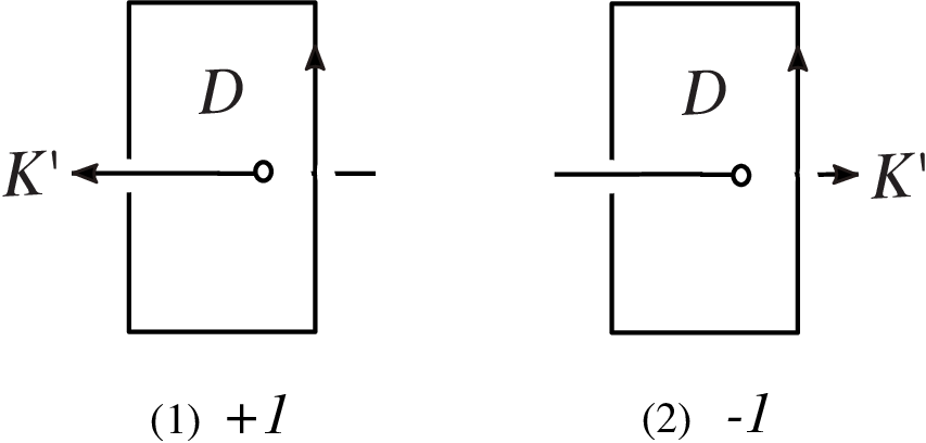
Refer to caption
Figure 8. Sign of the point of intersection: +1+1 in (1) and −1-1 in (2).
Refer to caption
Figure 9. F:=FbF:=F_{b} and E:=E(b,i)E:=E_{(b,i)}. (1) Subcone C(b,i)C_{(b,i)}. (2)(3) Possible shapes of 𝒞∩{x[F]+y[E]|x,y∈ℝ}\mathcal{C}\cap\{x[F]+y[E]\ |\ x,y\in{\mathbb{R}}\}. In case (2), [E]∈𝒞[E]\in\mathcal{C}. In case (3), [E]∉𝒞[E]\notin\mathcal{C}.

Definitions of ii-increasing braids, signs and intersection numbers

Let LL be an oriented link in S3S^{3} with a trivial component KK. We take an oriented disk DD bounded by the longitude of 𝒩⁡(K)\mathcal{N}(K) so that the orientation of DD agrees with the orientation of KK. For each component K′K^{\prime} of L−KL-K such that DD and K′K^{\prime} intersect transversally with D∩K′≠∅D\cap K^{\prime}\neq\emptyset, we assign each point of intersection +1+1 or −1-1 as shown in Figure 8.

Let bb be a braid with πb​(i)=i\pi_{b}(i)=i. We consider an oriented disk D=D(b,i)D=D_{(b,i)} bounded by the longitude ℓi\ell_{i} of 𝒩⁡(cl⁡(b⁡(i)))\mathcal{N}(\mathrm{cl}(b(i))). Such a disk DD is unique up to isotopy on ℰ⁡(cl⁡(b⁡(i)))\mathcal{E}(\mathrm{cl}(b(i))). We say that a braid b∈Bnb\in B_{n} with πb​(i)=i\pi_{b}(i)=i is ii-increasing (resp. ii-decreasing) if there is a disk D=D(b,i)D=D_{(b,i)} as above with the following conditions.

  1. (D1)

    There is at least one component K′K^{\prime} of cl⁡(b−b⁡(i))\mathrm{cl}(b-b(i)) such that D∩K′≠∅D\cap K^{\prime}\neq\emptyset.

  2. (D2)

    Each component of cl⁡(b−b⁡(i))\mathrm{cl}(b-b(i)) and DD intersect with each other transversally, and every point of intersection has the sign +1+1 (resp. −1-1).

We set ϵ⁡(b,i)=1\epsilon(b,i)=1 (resp. ϵ⁡(b,i)=−1\epsilon(b,i)=-1), and call it the sign of the pair (b,i)(b,i). We also call DD the associated disk of the pair (b,i)(b,i). We say that bb is ii-monotonic if bb is ii-increasing or ii-decreasing. Then we set

I⁡(b,i)=D∩cl⁡(b−b⁡(i))I(b,i)=D\cap\mathrm{cl}(b-b(i))

and let u⁡(b,i)≥1u(b,i)\geq 1 be the cardinality of I⁡(b,i)I(b,i). We call u⁡(b,i)u(b,i) the intersection number of the pair (b,i)(b,i). If the pair (b,i)(b,i) is specified, then we simply denote ϵ⁡(b,i)\epsilon(b,i) and u⁡(b,i)u(b,i) by ϵ\epsilon and uu respectively. For example σ12​σ2−1\sigma_{1}^{2}\sigma_{2}^{-1} is 11-increasing with u⁡(σ12​σ2−1,1)=1u(\sigma_{1}^{2}\sigma_{2}^{-1},1)=1.

A braid bb is positive if bb is represented by a word in letters σj\sigma_{j}, but not σj−1\sigma_{j}^{-1}. A braid bb is irreducible if the Nielsen-Thurston type of bb is not reducible.

Lemma 3.1.

Let bb be a positive braid with πb​(i)=i\pi_{b}(i)=i. Then bb is ii-increasing if bb is irreducible.

Proof.

Suppose that a positive braid bb with πb​(i)=i\pi_{b}(i)=i is irreducible. Since bb is positive, there is a disk D=D(b,i)D=D_{(b,i)} with the condition (D​2)(D2). Assume that DD fails in (D​1)(D1). Let ∂Dn\partial D_{n} be the boundary of the disk DnD_{n} containing nn punctures. Consider a neighborhood of ∂Dn∪(Dn∩D)\partial D_{n}\cup(D_{n}\cap D) in DnD_{n} which is an annulus. One of the boundary components of this annulus is an essential simple closed curve in DnD_{n} preserved by Γ⁡(b)∈Mod⁡(Dn)\Gamma(b)\in\mathrm{Mod}(D_{n}). This means that bb is reducible, a contradiction. Thus DD satisfies (D​1)(D1), and bb is ii-increasing. ∎

Orientation of the axis AA

Let bb be ii-monotonic with ϵ⁡(b,i)=ϵ\epsilon(b,i)=\epsilon and u⁡(b,i)=uu(b,i)=u. Consider the braided link br⁡(b)=cl⁡(b)∪A\mathrm{br}(b)=\mathrm{cl}(b)\cup A. The associated disk DD has a unique point of intersection with AA, and the cardinality of I⁡(b,i)∪(D∩A)I(b,i)\cup(D\cap A) is u⁡(b,i)+1u(b,i)+1. To deal with br⁡(b)=cl⁡(b)∪A\mathrm{br}(b)=\mathrm{cl}(b)\cup A as an oriented link, we consider an orientation of cl⁡(b)\mathrm{cl}(b) as we described before, and assign an orientation of AA so that the sign of the intersection between DD and AA coincides with ϵ⁡(b,i)\epsilon(b,i). See Figure 2(2).

Recall that Mb=ℰ⁡(br⁡(b))M_{b}=\mathcal{E}(\mathrm{br}(b)) is the exterior of br⁡(b)\mathrm{br}(b) which is a surface bundle over S1S^{1}. We consider an orientation of the FF-surface FbF_{b} which agrees with the orientation of AA.

EE-surface

We now define an oriented surface E(b,i)E_{(b,i)} of genus 00 embedded in MbM_{b}. Consider small u⁡(b,i)+1u(b,i)+1 disks in the oriented disk D=D(b,i)D=D_{(b,i)} whose centers are points of I⁡(b,i)∪(D∩A)I(b,i)\cup(D\cap A). Then E(b,i)E_{(b,i)} is a sphere with u⁡(b,i)+2u(b,i)+2 boundary components obtained from DD by removing the interiors of those small disks. We choose the orientation of E(b,i)E_{(b,i)} so that it agrees with the orientation of DD. We call E(b,i)E_{(b,i)} the EE-surface for bb. For example, the 11-increasing braid σ12​σ2−1\sigma_{1}^{2}\sigma_{2}^{-1} has the EE-surface E(σ12​σ2−1,1)E_{(\sigma_{1}^{2}\sigma_{2}^{-1},1)} homeomorphic to a 33-holed sphere.

Subcone C(b,i)C_{(b,i)}

Let us consider the 22-dimensional subcone C(b,i)C_{(b,i)} of H2​(Mb,∂Mb,ℝ)H_{2}(M_{b},\partial M_{b};{\mathbb{R}}) spanned by [Fb][F_{b}] and [E(b,i)][E_{(b,i)}] (Figure 9):

C(b,i)={x[Fb]+y[E(b,i)]|x>0,y>0}.C_{(b,i)}=\{x[F_{b}]+y[E_{(b,i)}]\ |\ x>0,\ y>0\}.

Let C(b,i)¯\overline{C_{(b,i)}} denote the closure of C(b,i)C_{(b,i)}. We write (x,y)=x⁡[Fb]+y⁡[E(b,i)](x,y)=x[F_{b}]+y[E_{(b,i)}]. We prove the following theorem in Section 4.

Theorem 3.2.

For a pseudo-Anosov, ii-increasing braid bb with u⁡(b,i)=uu(b,i)=u, let 𝒞\mathcal{C} be the fibered cone containing [Fb][F_{b}]. We have the following.

  1. (1)

    C(b,i)⊂𝒞C_{(b,i)}\subset\mathcal{C}.

  2. (2)

    The fiber F(x,y)F_{(x,y)} for each primitive integral class (x,y)∈C(b,i)(x,y)\in C_{(b,i)} has genus 00.

  3. (3)

    The monodromy ϕ(x,y):F(x,y)→F(x,y)\phi_{(x,y)}:F_{(x,y)}\rightarrow F_{(x,y)} for each primitive integral class (x,y)∈C(b,i)(x,y)\in C_{(b,i)} is conjugate to

    (ω1ψ)⋯(ωu−1ψ)(ωuψ)ψm−1:F(x,y)→F(x,y),(\omega_{1}\psi)\cdots(\omega_{u-1}\psi)(\omega_{u}\psi)\psi^{m-1}:F_{(x,y)}\rightarrow F_{(x,y)},

    where m≥1m\geq 1 depends on (x,y)(x,y), ψ\psi is periodic and each ωj\omega_{j} is reducible. Moreover there are homeomorphisms ω^j:S0→S0\widehat{\omega}_{j}:S_{0}\rightarrow S_{0} for j=1,…,uj=1,\ldots,u on a surface S0S_{0} determined by bb and an embedding h:S0↪F(x,y)h:S_{0}\hookrightarrow F_{(x,y)} such that the subsurface h⁡(S0)h(S_{0}) of F(x,y)F_{(x,y)} is the support of each wjw_{j} and

    wj|h⁡(S0)=h∘ω^j∘h−1.w_{j}|_{h(S_{0})}=h\circ\widehat{\omega}_{j}\circ h^{-1}.

The conclusion of Theorem 3.2 holds for ii-decreasing braids as well. We now claim that Theorem 3.2 implies Theorem B.

Proof of Theorem B.

Suppose that Theorem 3.2 holds. Let b∈Bnb\in B_{n} be a pseudo-Anosov braid such that πb​(i)=i\pi_{b}(i)=i. We consider the braid b​Δ2​k∈Bnb\Delta^{2k}\in B_{n} for k≥1k\geq 1. The full twist Δ2\Delta^{2} is an element in the center Z⁡(Bn)Z(B_{n}) and Δ2=σj​Pj\Delta^{2}=\sigma_{j}P_{j} holds for each 1≤j≤n−11\leq j\leq n-1, where PjP_{j} is positive. Such properties imply that b​Δ2​kb\Delta^{2k} is positive for kk large. We fix such large kk. Since Γ⁡(b)=Γ⁡(b​Δ2​k)\Gamma(b)=\Gamma(b\Delta^{2k}) in Mod⁡(Dn)\mathrm{Mod}(D_{n}), the braid b​Δ2​kb\Delta^{2k} is certainly pseudo-Anosov. Hence it is ii-increasing by Lemma 3.1. One can apply Theorem 3.2 for this braid, and obtains the subcone C(b​Δ2​k,i)C_{(b\Delta^{2k},i)}. Consider the kkth power of the disk twist about the disk DAD_{A} bounded by the longitude of 𝒩⁡(A)\mathcal{N}(A):

TDAk:ℰ⁡(A)→ℰ⁡(A).T_{D_{A}}^{k}:\mathcal{E}(A)\rightarrow\mathcal{E}(A).

Since A∪TDAk​(cl⁡(b))=A∪cl⁡(b​Δ2​k)=br⁡(b​Δ2​k)A\cup T_{D_{A}}^{k}(\mathrm{cl}(b))=A\cup\mathrm{cl}(b\Delta^{2k})=\mathrm{br}(b\Delta^{2k}), we have S3∖br⁡(b)≃S3∖br⁡(b​Δ2​k)S^{3}\setminus\mathrm{br}(b)\simeq S^{3}\setminus\mathrm{br}(b\Delta^{2k}). Let us set

fk:=hDA,k:Mb→Mb​Δ2​k,f_{k}:=h_{D_{A},k}:M_{b}\rightarrow M_{b\Delta^{2k}},

where hDA,kh_{D_{A},k} is the homeomorphism in (2.1). The isomorphism

fk∗:H2​(Mb,∂Mb)→H2​(Mb​Δ2​k,∂Mb​Δ2​k){f_{k}}_{*}:H_{2}(M_{b},\partial M_{b})\rightarrow H_{2}(M_{b\Delta^{2k}},\partial M_{b\Delta^{2k}})

sends [Fb][F_{b}] to [Fb​Δ2​k][F_{b\Delta^{2k}}]. (Here we note that the above kk is suppose to be large, but the homeomorphism fkf_{k} makes sense for all integer kk.) The pullback of the subcone C(b​Δ2​k,i)C_{(b\Delta^{2k},i)} into H2​(Mb,∂Mb)H_{2}(M_{b},\partial M_{b}) is a desired subcone contained in 𝒞\mathcal{C}. ∎

Remark 3.3.

If F(x,y)F_{(x,y)} is a (d+1)(d+1)-holed sphere, then the periodic homeomorphism ψ:F(x,y)→F(x,y)\psi:F_{(x,y)}\rightarrow F_{(x,y)} in Theorem 3.2 is determined by the periodic braid ρ=σ1​σ2​…​σd−2​σd−12∈Bd\rho=\sigma_{1}\sigma_{2}\ldots\sigma_{d-2}\sigma_{d-1}^{2}\in B_{d}. See the proof of Theorem 3.2(3) in Section 4.3.

4. Proof of Theorem 3.2

Refer to caption
Figure 10. (1) A0,…,AnA_{0},\ldots,A_{n}, QiQ_{i}, rir_{i} when n=3n=3, i=1i=1. (2) ∂D=ℓi\partial D=\ell_{i} is a union of four segments. UiU_{i} is an annulus in the figure.

We fix integers n≥3n\geq 3 and 1≤i≤n1\leq i\leq n. Throughout Section 4, we assume that b∈Bnb\in B_{n} is pseudo-Anosov and ii-increasing with u⁡(b,i)=uu(b,i)=u. We now choose an associated disk about the pair (b,i)(b,i) suitably. Let 𝔻{\mathbb{D}} denote the unit disk with the center (0,0)(0,0) in the plane ℝ2{\mathbb{R}}^{2}. Let J=(−1,1)×{0}⊂𝔻J=(-1,1)\times\{0\}\subset{\mathbb{D}} be the interval and let A0=(−2,0)A_{0}=(-2,0) be a point in ℝ2{\mathbb{R}}^{2}. We denote by 𝔻n{\mathbb{D}}_{n}, the disk 𝔻{\mathbb{D}} with equally spaced nn points in JJ. Let us denote these nn points by A1,…,AnA_{1},\ldots,A_{n} from left to right. We take a point Qi≠Ai∈JQ_{i}\neq A_{i}\in J between Ai−1A_{i-1} and AiA_{i} so that the Euclidean distance d⁡(Qi,Ai)d(Q_{i},A_{i}) is sufficiently small (e.g. d⁡(Qi,Ai)<1n+1d(Q_{i},A_{i})<\frac{1}{n+1}). Let rir_{i} denote the closed interval in [−2,1]×{0}[-2,1]\times\{0\} with endpoints A0A_{0} and QiQ_{i}. (Figure 10(1).) We regard bb as a braid contained in the cylinder 𝔻2×[0,1]⊂ℝ3{\mathbb{D}}^{2}\times[0,1]\subset{\mathbb{R}}^{3} and bb is based at nn points A1×{0},…,An×{0}A_{1}\times\{0\},\ldots,A_{n}\times\{0\}. Since πb​(i)=i\pi_{b}(i)=i, one can take a representative of bb such that b⁡(i)b(i) is an interval in the cylinder:

  1. ♢​1\diamondsuit 1.

    b⁡(i)=⋃0≤t≤1Ai×{t}b(i)=\displaystyle\bigcup_{0\leq t\leq 1}A_{i}\times\{t\}.

Furthermore we may assume that ∂D(=ℓi)\partial D(=\ell_{i}) of an associated disk DD of (b,i)(b,i) is a union of the following four segments as a set (Figure 10):

  1. ♢​2\diamondsuit 2.

    (⋃−1≤t≤2A0×{t})∪(ri×{−1})∪(⋃−1≤t≤2Qi×{t})∪(ri×{2})\bigl(\displaystyle\bigcup_{-1\leq t\leq 2}A_{0}\times\{t\}\bigr)\cup\bigl(r_{i}\times\{-1\}\bigr)\cup\bigl(\displaystyle\bigcup_{-1\leq t\leq 2}Q_{i}\times\{t\}\bigr)\cup\bigl(r_{i}\times\{2\}\bigr).

Preserving ♢​1,2\diamondsuit 1,2 we may further assume the following (Figures 10(2), 11(1)):

  1. ♢​3\diamondsuit 3.

    For a regular neighborhood UiU_{i} of ℓi\ell_{i} in DD, we have I⁡(b,i)⊂UiI(b,i)\subset U_{i}.

This is because every point x∈D∩K′x\in D\cap K^{\prime}, where K′K^{\prime} is a component of cl⁡(b−b⁡(i))\mathrm{cl}(b-b(i)), one can slide xx along K′K^{\prime} so that the resulting point on K′K^{\prime} is in UiU_{i}. Said differently, preserving ∂D\partial D pointwise, we can modify a small neighborhood of DD near K′K^{\prime} so that the resulting associated disk satisfies ♢​3\diamondsuit 3.

Under the conditions ♢​1,2,3\diamondsuit 1,2,3 we have the following. For each x∈D∩K′⊂Uix\in D\cap K^{\prime}\subset U_{i}, there is a segment s′⊂K′s^{\prime}\subset K^{\prime} through xx such that s′s^{\prime} passes over b⁡(i)b(i) since bb is ii-increasing. See Figure 11(1). Such a local picture of cl⁡(b)\mathrm{cl}(b) is used in the the next section. Hereafter we assume that associated disks possess conditions ♢​1,2,3\diamondsuit 1,2,3.

4.1. Proof of Theorem 3.2(1)

Let ss be the open segment in H2​(Mb,∂Mb,ℝ)H_{2}(M_{b},\partial M_{b};{\mathbb{R}}) with the endpoints n−1u​[E(b,i)]=(0,n−1u)\tfrac{n-1}{u}[E_{(b,i)}]=(0,\tfrac{n-1}{u}) and [Fb]=(1,0)[F_{b}]=(1,0):

(4.1) s={(x,y)∈C(b,i)|y=−n−1ux+n−1u, 0<x<1}.s=\{(x,y)\in C_{(b,i)}\ |\ y=-\dfrac{n-1}{u}x+\dfrac{n-1}{u},\ 0<x<1\}.

The ray of each point in C(b,i)C_{(b,i)} through the origin intersects with ss. Thus for the proof of (1), it suffices to prove that s⊂𝒞s\subset\mathcal{C}.

Refer to caption
Figure 11. Case: bb is ii-increasing. (1) Associated disk DD with conditions ♢\diamondsuit 1,2,3. (2) br⁡(b1)\mathrm{br}(b_{1}). Circles ∘\circ indicate points of intersection between DD and components of br⁡(b−b⁡(i))\mathrm{br}(b-b(i)). See also Figure 12.
Refer to caption
Figure 12. Braided links for (1) 11-increasing σ12​σ2−1\sigma_{1}^{2}\sigma_{2}^{-1}, (2) 22-increasing (σ12​σ2−1)1(\sigma_{1}^{2}\sigma_{2}^{-1})_{1} and (3) 33-increasing (σ12​σ2−1)2(\sigma_{1}^{2}\sigma_{2}^{-1})_{2}.

We now introduce a sequence of braided links {br⁡(bp)}p=1∞\{\mathrm{br}(b_{p})\}_{p=1}^{\infty} from an ii-increasing braid b∈Bnb\in B_{n} such that Mbp≃MbM_{b_{p}}\simeq M_{b} for each p≥1p\geq 1. (We use the 11-increasing braid σ12​σ2−1∈B3\sigma_{1}^{2}\sigma_{2}^{-1}\in B_{3} to illustrate the idea.) Let DD be an associated disk of the pair (b,i)(b,i). We take a disk twist

TD:ℰ⁡(cl⁡(b⁡(i)))→ℰ⁡(cl⁡(b⁡(i)))T_{D}:\mathcal{E}(\mathrm{cl}(b(i)))\rightarrow\mathcal{E}(\mathrm{cl}(b(i)))

so that the point of intersection D∩AD\cap A becomes the center of the twisting about DD, i.e. TD​(D∩A)=D∩AT_{D}(D\cap A)=D\cap A. We may assume that TD​(A)=AT_{D}(A)=A as a set. Figure 11 illustrates the image of the segment s′s^{\prime} under TDT_{D}. The condition ♢​3\diamondsuit 3 ensures that TDT_{D} equals the identity map outside a neighborhood of UiU_{i} in ℰ⁡(cl⁡(b⁡(i)))\mathcal{E}(\mathrm{cl}(b(i))). Then by ♢​1,2\diamondsuit 1,2, it follows that

TD​(br⁡(b−b⁡(i)))∪cl⁡(b⁡(i))T_{D}(\mathrm{br}(b-b(i)))\cup\mathrm{cl}(b(i))

is a braided link of some (i+u)(i+u)-increasing braid with (n+u)(n+u) strands. We define b1∈Bn+ub_{1}\in B_{n+u} to be such a braid. The trivial knot TD​(A)(=A)T_{D}(A)(=A) becomes a braid axis of b1b_{1}. By definition of the disk twist, we have Mb1≃MbM_{b_{1}}\simeq M_{b}. See Figure 12 for br⁡((σ12​σ2−1)1)\mathrm{br}((\sigma_{1}^{2}\sigma_{2}^{-1})_{1}).

As discussed below, there is some ambiguity in defining b1b_{1}. As we will see, the ambiguity is irrelevant for the study of pseudo-Anosov monodromies defined on fibers of fibrations on the mapping torus. Suppose that both DD and D′D^{\prime} are the associated disks of the pair (b,i)(b,i) with conditions ♢​1,2,3\diamondsuit 1,2,3. We consider the disk twists TDT_{D} and TD′T_{D^{\prime}} with the above condition, i.e. both D∩AD\cap A and D′∩AD^{\prime}\cap A become the center of the twisting about DD and D′D^{\prime} respectively. Observe that the resulting two links obtained from DD and D′D^{\prime} are equivalent:

TD​(br⁡(b−b⁡(i)))∪cl⁡(b⁡(i))∼TD′​(br⁡(b−b⁡(i)))∪cl⁡(b⁡(i)).T_{D}(\mathrm{br}(b-b(i)))\cup\mathrm{cl}(b(i))\sim T_{D^{\prime}}(\mathrm{br}(b-b(i)))\cup\mathrm{cl}(b(i)).

They are braided links, say br⁡(b1)\mathrm{br}(b_{1}) and br⁡(b1′)\mathrm{br}(b^{\prime}_{1}) of some braids b1,b1′∈Bn+ub_{1},b_{1}^{\prime}\in B_{n+u} respectively with the same axis TD​(A)=A=TD′​(A)T_{D}(A)=A=T_{D^{\prime}}(A). This means that a more stronger claim holds:

(br⁡(b1),A)∼(br⁡(b1′),A).(\mathrm{br}(b_{1}),A)\sim(\mathrm{br}(b^{\prime}_{1}),A).

Thus b1b_{1} and b1′b_{1}^{\prime} are conjugate in Bn+uB_{n+u} by Theorem 2.1. In particular both b1b_{1} and b1′b_{1}^{\prime} are pseudo-Anosov (since the initial braid bb is pseudo-Anosov and MbM_{b} is hyperbolic) and they have the same dilatation.

To define bpb_{p} for p≥1p\geq 1, we consider the ppth power

TDp:ℰ⁡(cl⁡(b⁡(i)))→ℰ⁡(cl⁡(b⁡(i)))T_{D}^{p}:\mathcal{E}(\mathrm{cl}(b(i)))\rightarrow\mathcal{E}(\mathrm{cl}(b(i)))

using the above TDT_{D}. As in the case of p=1p=1,

TDp​(br⁡(b−b⁡(i)))∪cl⁡(b⁡(i))T_{D}^{p}(\mathrm{br}(b-b(i)))\cup\mathrm{cl}(b(i))

is a braided link of some (i+p​u)(i+pu)-increasing braid with (n+p​u)(n+pu) strands. We define bp∈Bn+p​ub_{p}\in B_{n+pu} to be such a braid. Then Mbp≃MbM_{b_{p}}\simeq M_{b}. As in the case of p=1p=1, such a braid bpb_{p} is well-defined up to conjugate. We say that bpb_{p} is obtained from bb by the disk twist. Clearly u⁡(bp,i+p​u)=u⁡(b,i)u(b_{p},i+pu)=u(b,i) for p≥1p\geq 1. See Figure 12.

Let us set

gp:=hD,p:Mb→Mbp,g_{p}:=h_{D,p}:M_{b}\rightarrow M_{b_{p}},

where hD,ph_{D,p} is the homeomorphism in (2.1). We consider the isomorphism

gp∗:H2​(Mb,∂Mb)→H2​(Mbp,∂Mbp).{g_{p}}_{*}:H_{2}(M_{b},\partial M_{b})\rightarrow H_{2}(M_{b_{p}},\partial M_{b_{p}}).
Lemma 4.1.

For each integer p≥1p\geq 1, gp∗{g_{p}}_{*} sends (0,1)∈C(b,i)¯(0,1)\in\overline{C_{(b,i)}} to (0,1)∈C(bp,i+p​u)¯(0,1)\in\overline{C_{(b_{p},i+pu)}}, and sends (1,p)∈C(b,i)¯(1,p)\in\overline{C_{(b,i)}} to (1,0)∈C(bp,i+p​u)¯(1,0)\in\overline{C_{(b_{p},i+pu)}}. In particular for integers x,y≥1x,y\geq 1 with y=x​p+ry=xp+r for 0≤r<p0\leq r<p, gp∗{g_{p}}_{*} sends (x,y)∈C(b,i)¯(x,y)\in\overline{C_{(b,i)}} to (x,r)∈C(bp,i+p​u)¯(x,r)\in\overline{C_{(b_{p},i+pu)}}.

Proof.

We consider the oriented sum F(x,y):=x​Fb+y​E(b,i)F_{(x,y)}:=xF_{b}+yE_{(b,i)}. This is an oriented surface embedded in MbM_{b}, and is obtained from the cut and past construction of parallel xx copies of FbF_{b} and parallel yy copies of E(b,i)E_{(b,i)}. The orientation of F(x,y)F_{(x,y)} agrees with those of FbF_{b} and E(b,i)E_{(b,i)}. We have [F(x,y)]=(x,y)∈C(b,i)[F_{(x,y)}]=(x,y)\in C_{(b,i)}. Then gpg_{p} sends E(b,i)E_{(b,i)} to E(bp,i+p​u)E_{(b_{p},i+pu)}, and sends F(1,p)F_{(1,p)} to FbpF_{b_{p}}. Thus gp∗{g_{p}}_{*} sends (0,1)(0,1) to (0,1)(0,1), and sends (1,p)(1,p) to (1,0)(1,0). This completes the proof. ∎

By the proof of Lemma 4.1, g1g_{1} sends F(1,1)=Fb+E(b,i)F_{(1,1)}=F_{b}+E_{(b,i)} to the fiber Fb1F_{b_{1}} of a fibration on MbM_{b} associated with (1,1)∈C(b,i)(1,1)\in C_{(b,i)}. Since the fibers F(1,1)F_{(1,1)} and FbF_{b} are norm-minimizing, E(b,i)E_{(b,i)} is also norm-minimizing.

Proof of Theorem 3.2(1).

We have ‖[Fb]‖=n−1\|[F_{b}]\|=n-1 and ‖[Fbp]‖=n+p​u−1\|[F_{b_{p}}]\|=n+pu-1 since FbF_{b} and FbpF_{b_{p}} are fibers, and ‖[E(b,i)]‖=u\|[E_{(b,i)}]\|=u since E(b,i)E_{(b,i)} is norm-minimizing. By Lemma 4.1, [Fbp]=(1,p)∈C(b,i)[F_{b_{p}}]=(1,p)\in C_{(b,i)}. Consider the rational class

cp:=n−1n+p​u−1​[Fbp]=(n−1n+p​u−1,p⁡(n−1)n+p​u−1).c_{p}:=\dfrac{n-1}{n+pu-1}[F_{b_{p}}]=\Bigl(\dfrac{n-1}{n+pu-1},\dfrac{p(n-1)}{n+pu-1}\Bigr).

Then ‖cp‖=n−1\|c_{p}\|=n-1 for p≥1p\geq 1. The ray of [Fbp][F_{b_{p}}] through the origin is contained in some fibered cone for each p≥1p\geq 1. We easily check that cpc_{p} lies on ss in (4.1). This means that three classes [Fb][F_{b}], cpc_{p} and cp+1c_{p+1} with the same Thurston norm are contained in 𝒞\mathcal{C}. Observe that the small segment s′s^{\prime} in ss connecting [Fb][F_{b}] and cp+1c_{p+1} contains cpc_{p}, and s′⊂𝒞s^{\prime}\subset\mathcal{C} since ∥⋅∥\|\cdot\| is linear on each fibered cone. Moreover cp→(0,n−1u)∈∂s⊂∂𝒞(b,i)c_{p}\to(0,\tfrac{n-1}{u})\in\partial s\subset\partial\mathcal{C}_{(b,i)} as p→∞p\to\infty. Putting all things together, we conclude that s⊂𝒞s\subset\mathcal{C}. This completes the proof. ∎

Remark 4.2.

From the proof of Theorem 3.2(1), one sees the following: If [E(b,i)]∈C(b,i)¯[E_{(b,i)}]\in\overline{C_{(b,i)}} is a fibered class, then [E(b,i)]∈𝒞[E_{(b,i)}]\in\mathcal{C}. Otherwise [E(b,i)]∈∂𝒞[E_{(b,i)}]\in\partial{\mathcal{C}}. See Figure 9(2)(3).

4.2. Proof of Theorem 3.2(2)

We start with a simple observation: Δ2∈Bn\Delta^{2}\in B_{n} is jj-increasing for each 1≤j≤n1\leq j\leq n, and u⁡(Δ2,j)=n−1u(\Delta^{2},j)=n-1 holds. The following lemma is immediate.

Lemma 4.3.

If b∈Bnb\in B_{n} is ii-increasing, then b​Δ2∈Bnb\Delta^{2}\in B_{n} is ii-increasing with u⁡(b​Δ2,i)=u⁡(b,i)+n−1u(b\Delta^{2},i)=u(b,i)+n-1.

We explain the idea of Theorem 3.2(2). Let DD be the associated disk of the pair (b,i)(b,i). We have two types of the disk twist. One is TDAk:ℰ⁡(A)→ℰ⁡(A)T_{D_{A}}^{k}:\mathcal{E}(A)\rightarrow\mathcal{E}(A) which appears in the proof of Theorem B in Section 3 and the other is TDp:ℰ⁡(cl⁡(b⁡(i)))→ℰ⁡(cl⁡(b⁡(i)))T_{D}^{p}:\mathcal{E}(\mathrm{cl}(b(i)))\rightarrow\mathcal{E}(\mathrm{cl}(b(i))). If kk and pp are positive, then we obtain the ii-increasing b​Δ2​kb\Delta^{2k} from the former type TDAkT_{D_{A}}^{k}, and another increasing braid bpb_{p} from the latter type TDpT_{D}^{p}. Since both resulting braids are increasing, we can further apply two types of the disk twist for the resulting braid. This is a key of the proof. Choosing two types of the disk twist alternatively, we get a sequence of increasing and pseudo-Anosov braids (since the initial braid bb is pseudo-Anosov). We shall see that the desired monodromies associated with primitive classes in C(b,i)C_{(b,i)} are given by these braids.

Let p1,…,pjp_{1},\ldots,p_{j} be integers such that p1≥0p_{1}\geq 0 and p2,…,pj≥1p_{2},\ldots,p_{j}\geq 1. Given an ii-increasing braid b∈Bnb\in B_{n} with u⁡(b,i)=uu(b,i)=u, we define an integer i⁡[p1,…,pj]≥1i[p_{1},\ldots,p_{j}]\geq 1 and an i⁡[p1,…,pj]i[p_{1},\ldots,p_{j}]-increasing braid b⁡[p1,…,pj]b[p_{1},\ldots,p_{j}] inductively as follows.

  • •

    If j=1j=1 and p1=0p_{1}=0, then i⁡[0]=ii[0]=i and b⁡[0]=bb[0]=b. If j=1j=1 and p1=p≥1p_{1}=p\geq 1, then i⁡[p]=i+p​ui[p]=i+pu and b⁡[p]=bpb[p]=b_{p}.

  • •

    If j>1j>1 is even, then

    i⁡[p1,…,pj−1,pj]\displaystyle i[p_{1},\ldots,p_{j-1},p_{j}] =\displaystyle= i⁡[p1,…,pj−1],\displaystyle i[p_{1},\ldots,p_{j-1}],
    b⁡[p1,…,pj−1,pj]\displaystyle b[p_{1},\ldots,p_{j-1},p_{j}] =\displaystyle= (b⁡[p1,…,pj−1])​Δ2​pj.\displaystyle\bigl(b[p_{1},\ldots,p_{j-1}]\bigr)\Delta^{2p_{j}}.

    The right-hand side is i⁡[p1,…,pj−1]i[p_{1},\ldots,p_{j-1}]-increasing by Lemma 4.3.

  • •

    If j>1j>1 is odd, then

    i⁡[p1,…,pj−1,pj]\displaystyle i[p_{1},\ldots,p_{j-1},p_{j}] =\displaystyle= i⁡[p1,…,pj−1]+pj​u​(b⁡[p1,…,pj−1],i⁡[p1,…,pj−1]),\displaystyle i[p_{1},\ldots,p_{j-1}]+p_{j}u\bigl(b[p_{1},\ldots,p_{j-1}],i[p_{1},\ldots,p_{j-1}]\bigr),
    b⁡[p1,…,pj−1,pj]\displaystyle b[p_{1},\ldots,p_{j-1},p_{j}] =\displaystyle= (b⁡[p1,…,pj−1])pj.\displaystyle\bigl(b[p_{1},\ldots,p_{j-1}]\bigr)_{p_{j}}.

We say that b⁡[p1,…,pj]b[p_{1},\ldots,p_{j}] has length jj.

Example 4.4.
  1. (1)

    b⁡[p]=bpb[p]=b_{p} by definition.

  2. (2)

    Let β=b​Δ2\beta=b\Delta^{2}. Then b⁡[0,1]=βb[0,1]=\beta and b⁡[0,1,p]=βpb[0,1,p]=\beta_{p}.

  3. (3)

    We have b⁡[0,p]=b​Δ2​pb[0,p]=b\Delta^{2p} and b⁡[0,p,1]=(b​Δ2​p)1b[0,p,1]=(b\Delta^{2p})_{1}, where (b​Δ2​p)1(b\Delta^{2p})_{1} is obtained from ii-increasing b​Δ2​pb\Delta^{2p} by the disk twist.

For each k≥1k\geq 1, let fk:Mb→Mb​Δ2​kf_{k}:M_{b}\rightarrow M_{b\Delta^{2k}} be the homeomorphism which in the proof of Theorem B. Consider the isomorphism fk∗:H2​(Mb,∂Mb)→H2​(Mb​Δ2​k,∂Mb​Δ2​k){f_{k}}_{*}:H_{2}(M_{b},\partial M_{b})\rightarrow H_{2}(M_{b\Delta^{2k}},\partial M_{b\Delta^{2k}}). We have the following property.

Lemma 4.5.

For each integer k≥1k\geq 1, fk∗{f_{k}}_{*} sends (1,0)∈C(b,i)¯(1,0)\in\overline{C_{(b,i)}} to (1,0)∈C(b​Δ2​k,i)¯(1,0)\in\overline{C_{(b\Delta^{2k},i)}}, and sends (k,1)∈C(b,i)¯(k,1)\in\overline{C_{(b,i)}} to (0,1)∈C(b​Δ2​k,i)¯(0,1)\in\overline{C_{(b\Delta^{2k},i)}}. In particular for integers x,y≥1x,y\geq 1 with x=y​k+rx=yk+r for 0≤r<k0\leq r<k, then fk∗{f_{k}}_{*} sends (x,y)∈C(b,i)¯(x,y)\in\overline{C_{(b,i)}} to (r,y)∈C(b​Δ2​k,i)¯(r,y)\in\overline{C_{(b\Delta^{2k},i)}}.

Proof.

The homeomorphism fkf_{k} sends FbF_{b} to Fb​Δ2​kF_{b\Delta^{2k}}, and sends F(k,1)=k​Fb+E(b,i)F_{(k,1)}=kF_{b}+E_{(b,i)} to E(b​Δ2​k,i)E_{(b\Delta^{2k},i)}. This implies that the claim holds. ∎

Proof of Theorem 3.2(2).

Let (x,y)∈C(b,i)(x,y)\in C_{(b,i)} be a primitive integral class. (Hence x,yx,y are positive integers with gcd⁡(x,y)=1\gcd(x,y)=1.) We consider the continued fraction of y/xy/x by the Euclidean algorithm

yx=p1+1p2+1p3+⋯+1pj−1+1pj:=p1+1p2​+​1p3​+⋯+​1pj−1​+​1pj​\frac{y}{x}=p_{1}+\cfrac{1}{p_{2}+\cfrac{1}{p_{3}+\cdots+\cfrac{1}{p_{j-1}+\cfrac{1}{p_{j}}}}}:=p_{1}+\frac{1}{p_{2}}{\genfrac{}{}{0.0pt}{}{}{+}}\frac{1}{p_{3}}{\genfrac{}{}{0.0pt}{}{}{+ \cdots+}}\frac{1}{p_{j-1}}{\genfrac{}{}{0.0pt}{}{}{+}}\frac{1}{p_{j}}{\genfrac{}{}{0.0pt}{}{}{}}

with length jj and pj≥2p_{j}\geq 2 and p1=0p_{1}=0 if 0<y<x0<y<x. There is another expression

yx=p1+1p2​+​1p3​+⋯+​1pj−1​+​1(pj−1)​+​11​\frac{y}{x}=p_{1}+\frac{1}{p_{2}}{\genfrac{}{}{0.0pt}{}{}{+}}\frac{1}{p_{3}}{\genfrac{}{}{0.0pt}{}{}{+ \cdots+}}\frac{1}{p_{j-1}}{\genfrac{}{}{0.0pt}{}{}{+}}\frac{1}{(p_{j}-1)}{\genfrac{}{}{0.0pt}{}{}{+}}\frac{1}{1}{\genfrac{}{}{0.0pt}{}{}{}}

with length j+1j+1. We choose one of the two expressions with odd length ℓ\ell:

yx=p1+1p2​+​1p3​+⋯+​1pℓ−1​+​1pℓ​.\frac{y}{x}=p_{1}+\frac{1}{p_{2}}{\genfrac{}{}{0.0pt}{}{}{+}}\frac{1}{p_{3}}{\genfrac{}{}{0.0pt}{}{}{+ \cdots+}}\frac{1}{p_{\ell-1}}{\genfrac{}{}{0.0pt}{}{}{+}}\frac{1}{p_{\ell}}{\genfrac{}{}{0.0pt}{}{}{}}.

This encodes the fiber F(x,y)F_{(x,y)} and its monodromy ϕ(x,y)\phi_{(x,y)}. In fact Lemmas 4.1, 4.5 ensure that

(gpℓfpℓ−1gpℓ−2⋯fp2gp1)∗:H2(Mb,∂Mb)→H2(Mb⁡[p1,…,pℓ],∂Mb⁡[p1,…,pℓ])(g_{p_{\ell}}f_{p_{\ell-1}}g_{p_{\ell-2}}\cdots f_{p_{2}}g_{p_{1}})_{*}:H_{2}(M_{b},\partial M_{b})\rightarrow H_{2}(M_{b[p_{1},\ldots,p_{\ell}]},\partial M_{b[p_{1},\ldots,p_{\ell}]})

sends (x,y)=[x​Fb+y​E(b,i)](x,y)=[xF_{b}+yE_{(b,i)}] to (1,0)(1,0) which is the integral class of the FF-surface of b⁡[p1,…,pℓ]b[p_{1},\ldots,p_{\ell}]. (gp1=i​d:Mb→Mbg_{p_{1}}=id:M_{b}\rightarrow M_{b} if p1=0p_{1}=0.) Thus F(x,y)F_{(x,y)} has genus 00. Moreover this means that one can take Fb⁡[p1,…,pℓ]F_{b[p_{1},\ldots,p_{\ell}]} as a representative of (x,y)∈C(b,i)(x,y)\in C_{(b,i)} and the monodromy ϕ(x,y):F(x,y)→F(x,y)\phi_{(x,y)}:F_{(x,y)}\rightarrow F_{(x,y)} is determined by b⁡[p1,…,pℓ]b[p_{1},\ldots,p_{\ell}]. This completes the proof. ∎

We denote by b(x,y)b_{(x,y)} the braid b⁡[p1,…,pℓ]b[p_{1},\ldots,p_{\ell}] which determines ϕ(x,y)\phi_{(x,y)}. Here is an example: If (x,y)=(5,14)(x,y)=(5,14), then 145=2+11​+​14​\frac{14}{5}=2+\frac{1}{1}{\genfrac{}{}{0.0pt}{}{}{+}}\frac{1}{4}{\genfrac{}{}{0.0pt}{}{}{}} and ϕ(5,14)\phi_{(5,14)} is determined by b(5,14)=b⁡[2,1,4]b_{(5,14)}=b[2,1,4]. If (x,y)=(14,5)(x,y)=(14,5), then 514=0+12​+​11​+​13​+​11​\frac{5}{14}=0+\frac{1}{2}{\genfrac{}{}{0.0pt}{}{}{+}}\frac{1}{1}{\genfrac{}{}{0.0pt}{}{}{+}}\frac{1}{3}{\genfrac{}{}{0.0pt}{}{}{+}}\frac{1}{1}{\genfrac{}{}{0.0pt}{}{}{}} and ϕ(14,5)\phi_{(14,5)} is determined by b(14,5)=b⁡[0,2,1,3,1]b_{(14,5)}=b[0,2,1,3,1].

4.3. Proof of Theorem 3.2(3)

We begin with the following lemma.

Lemma 4.6 (Standard form).

If b∈Bnb\in B_{n} is ii-increasing with u⁡(b,i)=uu(b,i)=u, then bb is conjugate to an nn-increasing braid b′b^{\prime} of the form

b′=(w1σn−12)⋯(wuσn−12),b^{\prime}=(w_{1}\sigma_{n-1}^{2})\cdots(w_{u}\sigma_{n-1}^{2}),

where each wkw_{k} is a word of σ1±1,…,σn−2±1\sigma_{1}^{\pm 1},\ldots,\sigma_{n-2}^{\pm 1}, but not σn−1±1\sigma_{n-1}^{\pm 1}, possibly wk=∅w_{k}=\emptyset for some kk.

Figure 13(1) shows the form of b′b^{\prime} in Lemma 4.6 in case u=2u=2.

Proof.

We regard bb as a braid in 𝔻×[0,1]{\mathbb{D}}\times[0,1]. By ♢​1\diamondsuit 1, b⁡(i)b(i) is an interval in 𝔻×[0,1]{\mathbb{D}}\times[0,1]. If i=ni=n, then bb is nn-increasing and it is not hard to see that a representative of bb is of the desired form in Lemma 4.6. Suppose that bb is ii-increasing for 1≤i<n1\leq i<n. We set σ=σn−1σn−2⋯σi\sigma=\sigma_{n-1}\sigma_{n-2}\cdots\sigma_{i} if 1≤i<n−11\leq i<n-1 and σ=σn−1\sigma=\sigma_{n-1} if i=n−1i=n-1. We consider the nn-braid b′=σ​b​σ−1b^{\prime}=\sigma b\sigma^{-1} which is nn-increasing with u⁡(b′,n)=uu(b^{\prime},n)=u. We pull b′​(n)b^{\prime}(n) tight in 𝔻×[0,1]{\mathbb{D}}\times[0,1] and make it straight. Then a representative of b′b^{\prime} is of the desired form. ∎

Refer to caption
Figure 13. The figure illustrates how an initial braid bb generates {bp}\{b_{p}\}. (1) b=w1​σ32​w2​σ32=(ν1​ρ)​(ν2​ρ)∈B4b=w_{1}\sigma_{3}^{2}w_{2}\sigma_{3}^{2}=(\nu_{1}\rho)(\nu_{2}\rho)\in B_{4}, where νj=wj​(σ1​σ2)−1\nu_{j}=w_{j}(\sigma_{1}\sigma_{2})^{-1}. (2) b1=(ν1​ρ)​(ν2​ρ)∈B6b_{1}=(\nu_{1}\rho)(\nu_{2}\rho)\in B_{6}. (3) b2=(ν1​ρ)​(ν2​ρ)∈B8b_{2}=(\nu_{1}\rho)(\nu_{2}\rho)\in B_{8}.
Proof of Theorem 3.2(3).

Since each ii-increasing braid is conjugate to an nn-increasing braid of a standard form in Lemma 4.6, we may assume that b∈Bnb\in B_{n} is an nn-increasing braid of the form b=(w1σn−12)⋯(wuσn−12)b=(w_{1}\sigma_{n-1}^{2})\cdots(w_{u}\sigma_{n-1}^{2}). Since ρ∈Bn\rho\in B_{n} is the periodic braid such that ρ=σ1σ2⋯σn−2σn−12\rho=\sigma_{1}\sigma_{2}\cdots\sigma_{n-2}\sigma_{n-1}^{2} we have σn−12=(σ1⋯σn−2)−1ρ\sigma_{n-1}^{2}=(\sigma_{1}\cdots\sigma_{n-2})^{-1}\rho. Then bb is expressed as follows.

b=(ν1ρ)⋯(νuρ),b=(\nu_{1}\rho)\cdots(\nu_{u}\rho),

where νi=wi(σ1⋯σn−2)−1\nu_{i}=w_{i}(\sigma_{1}\cdots\sigma_{n-2})^{-1} is written by a word of σ1±1,⋯,σn−2±1\sigma_{1}^{\pm 1},\cdots,\sigma_{n-2}^{\pm 1}, but not σn−1±1\sigma_{n-1}^{\pm 1}. Each νj\nu_{j} in bb is a reducible braid and ρ\rho in bb is the periodic braid. Let ωj:Fb→Fb\omega_{j}:F_{b}\rightarrow F_{b} denote a reducible representative whose mapping class is determined by νj\nu_{j}, and let ψ:Fb→Fb\psi:F_{b}\rightarrow F_{b} denote a periodic representative whose mapping class determined by ρ\rho. The monodromy ϕb\phi_{b} defined on FbF_{b} is written by ϕb=(ω1ψ)⋯(ωuψ)\phi_{b}=(\omega_{1}\psi)\cdots(\omega_{u}\psi).

Recall that 𝔻n−1{\mathbb{D}}_{n-1} is the disk 𝔻{\mathbb{D}} with marked points A1,⋯,An−1A_{1},\cdots,A_{n-1}. Let S0S_{0} be an nn-holed sphere obtained from 𝔻n−1{\mathbb{D}}_{n-1} by removing the interiors of small (n−1)(n-1) disks with centers A1,⋯,An−1A_{1},\cdots,A_{n-1}. Each νj\nu_{j} as an (n−1)(n-1)-braid determines a homeomorphism ω^j:S0→S0\widehat{\omega}_{j}:S_{0}\rightarrow S_{0}. We may assume that ω^j\widehat{\omega}_{j} fixes one of the boundary components corresponding to ∂𝔻\partial{\mathbb{D}} pointwise. It is clear that we have an embedding h:S0↪Fbh:S_{0}\hookrightarrow F_{b} such that each ωj\omega_{j} in ϕb\phi_{b} is reducible supported on the subsurface h⁡(S0)h(S_{0}) and the restriction of ωj\omega_{j} to h⁡(S0)h(S_{0}) is given by h∘ω^j∘h−1h\circ\widehat{\omega}_{j}\circ h^{-1}.

By the proof of Theorem 3.2(2), ϕ(x,y):F(x,y)→F(x,y)\phi_{(x,y)}:F_{(x,y)}\rightarrow F_{(x,y)} associated with each primitive class (x,y)∈C(b,i)(x,y)\in C_{(b,i)} is determined by the braid of the form b⁡[p1,…,pℓ]b[p_{1},\ldots,p_{\ell}]. We now prove by the induction on length ℓ\ell that

b[p1,…,pℓ]=(ν1ρ)⋯(νu−1ρ)(νuρ)ρm−1=(ν1ρ)⋯(νu−1ρ)(νuρm)b[p_{1},\ldots,p_{\ell}]=(\nu_{1}\rho)\cdots(\nu_{u-1}\rho)(\nu_{u}\rho)\rho^{m-1}=(\nu_{1}\rho)\cdots(\nu_{u-1}\rho)(\nu_{u}\rho^{m})

for some m≥1m\geq 1 depending on (x,y)(x,y). Here each νj\nu_{j} in b⁡[p1,…,pℓ]b[p_{1},\ldots,p_{\ell}] is a reducible braid which is an extension of νj\nu_{j} in bb and ρ\rho is the periodic braid with the degree of b⁡[p1,…,pj]b[p_{1},\ldots,p_{j}]. If this holds, then ϕ(x,y)\phi_{(x,y)} has a desired property as in Theorem 3.2(3). Suppose that ℓ=1\ell=1. If p1=0p_{1}=0, then b⁡[0]=bb[0]=b and we are done. If p1≥1p_{1}\geq 1, then b⁡[p1]=bp1b[p_{1}]=b_{p_{1}}. Using the above expression of bb we observe that bp1b_{p_{1}} is written by

bp1=(ν1ρ)⋯(νuρ)∈Bn+p1​ub_{p_{1}}=(\nu_{1}\rho)\cdots(\nu_{u}\rho)\in B_{n+p_{1}u}

(see Figure 13). We are done.

For ℓ≥2\ell\geq 2, suppose that b[p1,…,pℓ−1]=(ν1ρd)⋯(νu−1ρd)(νuρdm)b[p_{1},\ldots,p_{\ell-1}]=(\nu_{1}\rho_{d})\cdots(\nu_{u-1}\rho_{d})(\nu_{u}\rho_{d}^{m}) for some mm, where dd is the degree of b⁡[p1,…,pℓ−1]b[p_{1},\ldots,p_{\ell-1}]. Consider b⁡[p1,…,pℓ]b[p_{1},\ldots,p_{\ell}] with length ℓ\ell. If ℓ\ell is even, then by induction hypothesis

b[p1,…,pℓ]=(b[p1,…,pℓ−1])Δd2​pℓ=(ν1ρd)⋯(νu−1ρd)(νuρdm)Δd2​pℓ.b[p_{1},\ldots,p_{\ell}]=\bigl(b[p_{1},\ldots,p_{\ell-1}]\bigr)\Delta_{d}^{2p_{\ell}}=(\nu_{1}\rho_{d})\cdots(\nu_{u-1}\rho_{d})(\nu_{u}\rho_{d}^{m})\Delta_{d}^{2p_{\ell}}.

Since Δd2=ρdd−1\Delta_{d}^{2}=\rho_{d}^{d-1} we have (νu​ρdm)​Δd2​pℓ=νu​ρdm+pℓ​(d−1)(\nu_{u}\rho_{d}^{m})\Delta_{d}^{2p_{\ell}}=\nu_{u}\rho_{d}^{m+p_{\ell}(d-1)}. Thus b⁡[p1,…,pℓ]b[p_{1},\ldots,p_{\ell}] has a desired expression and we are done. If ℓ\ell is odd, then by induction hypothesis again

b[p1,…,pℓ]=(b[p1,…,pℓ−1])pℓ=((ν1ρd)⋯(νu−1ρd)(νuρdm))pℓ.b[p_{1},\ldots,p_{\ell}]=\bigr(b[p_{1},\ldots,p_{\ell-1}]\bigl)_{p_{\ell}}=\bigl((\nu_{1}\rho_{d})\cdots(\nu_{u-1}\rho_{d})(\nu_{u}\rho_{d}^{m})\bigr)_{p_{\ell}}.

As in the case of ℓ=1\ell=1, the braid in the right-hand side is expressed as

((ν1ρd)⋯(νu−1ρd)(νuρdm))pℓ=(ν1ρ†)⋯(νu−1ρ†)(νuρ†m),\bigl((\nu_{1}\rho_{d})\cdots(\nu_{u-1}\rho_{d})(\nu_{u}\rho_{d}^{m})\bigr)_{p_{\ell}}=(\nu_{1}\rho_{{\dagger}})\cdots(\nu_{u-1}\rho_{{\dagger}})(\nu_{u}\rho_{{\dagger}}^{m}),

where †{\dagger} is the degree of b⁡[p1,…,pℓ]b[p_{1},\ldots,p_{\ell}]. This completes the proof. ∎

5. Sequences of pseudo-Anosov braids with small normalized entropies

In this section we prove Theorem A. We begin with an observation. Let Ω⊂{a∈𝒞|‖a‖=1}\Omega\subset\{a\in\mathcal{C}\ |\ \|a\|=1\} be a compact set in H2​(Mb,∂Mb,ℝ)H_{2}(M_{b},\partial M_{b};{\mathbb{R}}) and let 𝒞Ω⊂𝒞\mathcal{C}_{\Omega}\subset\mathcal{C} denote the cone over Ω\Omega through the origin. By Theroem 2.3(2) there is a constant P=P⁡(Ω)>0P=P(\Omega)>0 depending on Ω\Omega such that Ent⁡(a)<P\mathrm{Ent}(a)<P for any a∈CΩa\in C_{\Omega}. This observation provides us many sequences of pseudo-Anosov braids with small normalized entropies from a single pseudo-Anosov braid bb.

Theorem 5.1.

Suppose that bb is a pseudo-Anosov braid whose permutation has a fixed point. We fix any 0<ℓ<∞0<\ell<\infty. Let {(xp,yp)}\{(x_{p},y_{p})\} be a sequence of primitive integral classes in C(b,i)C_{(b,i)} such that yp/xp<ℓy_{p}/x_{p}<\ell and ‖(xp,yp)‖≍p\|(x_{p},y_{p})\|\asymp p. Then the sequence of pseudo-Anosov braids {b(xp,yp)}\{b_{(x_{p},y_{p})}\} has a small normalized entropy.

Proof.

If {(xp,yp)}\{(x_{p},y_{p})\} is the sequence under the assumption, then we have d⁡(b(xp,yp))≍‖(xp,yp)‖≍pd(b_{(x_{p},y_{p})})\asymp\|(x_{p},y_{p})\|\asymp p. Since (1,0)∈C(b,i)⊂𝒞(1,0)\in C_{(b,i)}\subset\mathcal{C} and the slope of yp/xpy_{p}/x_{p} is bounded by ℓ\ell from above, the set of projective classes (xp,yp)(x_{p},y_{p}) is contained in some compact set in {a∈𝒞|‖a‖=1}\{a\in\mathcal{C}\ |\ \|a\|=1\} (Figure 9). Thus there is a constant P=P⁡(ℓ)>1P=P(\ell)>1 such that Ent⁡(b(xp,yp))<P\mathrm{Ent}(b_{(x_{p},y_{p})})<P for any pp. This completes the proof. ∎

Let us discuss three sequences coming from Example 4.4. They are {bp}\{b_{p}\}, {βp}\{\beta_{p}\} and {(b​Δ2​p)1}\{(b\Delta^{2p})_{1}\} varying pp. It is not hard to see that d⁡(bp)d(b_{p}), d⁡(βp)d(\beta_{p}), d⁡((b​Δ2​p)1)≍pd((b\Delta^{2p})_{1})\asymp p.

Theorem 5.2.

For an ii-increasing and pseudo-Anosov b∈Bnb\in B_{n}, we have the following on the sequences of pseudo-Anosov braids.

  1. (1)

    {bp}\{b_{p}\} has a small normalized entropy if and only if [E(b,i)][E_{(b,i)}] is a fibered class.

  2. (2)

    For β=b​Δ2∈Bn\beta=b\Delta^{2}\in B_{n}, {βp}\{\beta_{p}\} has a small normalized entropy and Ent⁡(βp)→Ent⁡((1,1))\mathrm{Ent}(\beta_{p})\to\mathrm{Ent}((1,1)) as p→∞p\to\infty.

  3. (3)

    {(b​Δ2​p)1}\{(b\Delta^{2p})_{1}\} has a small normalized entropy and Ent⁡((b​Δ2​p)1)→Ent⁡(b)\mathrm{Ent}((b\Delta^{2p})_{1})\to\mathrm{Ent}(b) as p→∞p\to\infty.

Proof of Theorem 5.2.

For a=(x,y)∈C(b,i)¯a=(x,y)\in\overline{C_{(b,i)}}, let a¯=(x,y)¯\underline{a}=\underline{(x,y)} denote its projective class. We have [Fbp]¯=(1,p)¯→[E(b,i)]¯=(0,1)¯\underline{[F_{b_{p}}]}=\underline{(1,p)}\to\underline{[E_{(b,i)}]}=\underline{(0,1)} as p→∞p\to\infty. If [E(b,i)][E_{(b,i)}] is a fibered class, then [E(b,i)]∈𝒞[E_{(b,i)}]\in\mathcal{C} by Remark 4.2 and Ent⁡(bp)→Ent⁡([E(b,i)])\mathrm{Ent}(b_{p})\to\mathrm{Ent}([E_{(b,i)}]) as p→∞p\to\infty by Theorem 2.3(2). If [E(b,i)][E_{(b,i)}] is a non-fibered class, then [E(b,i)]∈∂𝒞[E_{(b,i)}]\in\partial\mathcal{C} by Remark 4.2, and Ent⁡(bp)→∞\mathrm{Ent}(b_{p})\to\infty as p→∞p\to\infty by Theorem 2.3(3). We finish the proof of (1). We turn to (2). Since [Fβp]=(p+1,p)∈C(b,i)[F_{\beta_{p}}]=(p+1,p)\in C_{(b,i)}, its projective class goes to (1,1)¯\underline{(1,1)} as p→∞p\to\infty. Since (1,1)∈C(b,i)⊂𝒞(1,1)\in C_{(b,i)}\subset\mathcal{C} by Theorem 3.2(1), Ent⁡(βp)→Ent⁡((1,1))\mathrm{Ent}(\beta_{p})\to\mathrm{Ent}((1,1)) as p→∞p\to\infty by Theorem 2.3(2). This completes the proof of (2). Finally we prove (3). The fibered class of FF-surface of (b​Δ2​p)1(b\Delta^{2p})_{1} is given by (p+1,1)∈C(b,i)(p+1,1)\in C_{(b,i)}. Its projective class goes to [Fb]¯=(1,0)¯\underline{[F_{b}]}=\underline{(1,0)} as p→∞p\to\infty. Thus Ent⁡((b​Δ2​p)1)→Ent⁡(b)\mathrm{Ent}((b\Delta^{2p})_{1})\to\mathrm{Ent}(b) as p→∞p\to\infty. This completes the proof. ∎

We use Theorem 5.2(1)(2) in Section 8. For an application using (3), see [19].

Proof of Theorem A.

Suppose that b∈Bnb\in B_{n} is pseudo-Anosov with πb​(i)=i\pi_{b}(i)=i. Let β⁡(k)\beta(k) denote b​Δ2​k∈Bnb\Delta^{2k}\in B_{n} for k≥1k\geq 1. Clearly β⁡(k)\beta(k) is pseudo-Anosov with the same dilatation as bb (for any kk) and β⁡(k)\beta(k) is positive for kk large. We fix such large kk. By Lemma 3.1 β⁡(k)\beta(k) is ii-increasing. If we let zp=(β⁡(k)​Δ2​p)1z_{p}=(\beta(k)\Delta^{2p})_{1}, then Mzp≃Mβ⁡(k)≃MbM_{z_{p}}\simeq M_{\beta(k)}\simeq M_{b} holds for p≥1p\geq 1. By Theorem 5.2(3), {zp}\{z_{p}\} has a small normalized entropy and Ent⁡(zp)→Ent⁡(β⁡(k))=Ent⁡(b)\mathrm{Ent}(z_{p})\to\mathrm{Ent}(\beta(k))=\mathrm{Ent}(b) as p→∞p\to\infty. ∎

Let bp∙b_{p}^{\bullet} denote the braid obtained from (i+p​u)(i+pu)-increasing bpb_{p} by removing the strand of the index i+p​ui+pu. Taking its spherical element we have S⁡(bp∙)S(b_{p}^{\bullet}). A mild generalization of the sequence {bp}\{b_{p}\} is the ones {bp∙}\{b_{p}^{\bullet}\} and {S⁡(bp∙)}\{S(b_{p}^{\bullet})\} varing pp. Although bp∙b_{p}^{\bullet}, S⁡(bp∙)S(b_{p}^{\bullet}) may not be pseudo-Anosov, they are frequently pseudo-Anosov. To be more precise, we need to consider the number of prongs of singularities in the stable foliation ℱbp\mathcal{F}_{b_{p}} for bpb_{p} as we explained in Section 2.3. This is the motivation of the study in Section 6

6. Stable foliation for the monodromy

Refer to caption
Figure 14. Case: bb is ii-increasing. (1) Meridian and longitude basis. (2) Two boundary slopes ∂(b,A)F(1,1)\partial_{(b,A)}F_{(1,1)} (in green) on 𝒯(b,A)\mathcal{T}_{(b,A)} and ∂(b,i)F(1,1)\partial_{(b,i)}F_{(1,1)} (in red) on 𝒯(b,i)\mathcal{T}_{(b,i)} when (x,y)=(1,1)(x,y)=(1,1).

Let bb be pseudo-Anosov and ii-monotonic with the sign ϵ⁡(b,i)=ϵ\epsilon(b,i)=\epsilon. For any primitive integral class (x,y)∈C(b,i)(x,y)\in C_{(b,i)}, the oriented sum F(x,y)=x​Fb+y​E(b,i)F_{(x,y)}=xF_{b}+yE_{(b,i)} is connected. Let 𝒯(b,A)\mathcal{T}_{(b,A)} and 𝒯(b,i)\mathcal{T}_{(b,i)} denote the tori ∂𝒩⁡(A)\partial\mathcal{N}(A) and ∂𝒩⁡(cl⁡(b⁡(i)))\partial\mathcal{N}(\mathrm{cl}(b(i))) respectively. Let us set

∂(b,A)F(x,y)=∂F(x,y)∩𝒯(b,A)​and​∂(b,i)F(x,y)=∂F(x,y)∩𝒯(b,i),\partial_{(b,A)}F_{(x,y)}=\partial F_{(x,y)}\cap\mathcal{T}_{(b,A)}\hskip 8.53581pt\mbox{and}\hskip 8.53581pt\partial_{(b,i)}F_{(x,y)}=\partial F_{(x,y)}\cap\mathcal{T}_{(b,i)},

each of which is a single simple closed curve on the torus (since gcd⁡(x,y)=1\gcd(x,y)=1). Recall that we chose the orientation of the axis for the ii-monotonic bb in Section 3. We use the meridian and longitude basis {mA,ℓA}\{m_{A},\ell_{A}\} for 𝒯(b,A)\mathcal{T}_{(b,A)} to represent a homology class of a disjoint union of simple closed curves on 𝒯(b,A)\mathcal{T}_{(b,A)}. We also use the meridian and the longitude basis {mi,ℓi}\{m_{i},\ell_{i}\} for 𝒯(b,i)\mathcal{T}_{(b,i)}. Observe that the homology classes [∂(b,A)F(x,y)][\partial_{(b,A)}F_{(x,y)}] and [∂(b,i)F(x,y)][\partial_{(b,i)}F_{(x,y)}] are given by the pairs of integers

(6.1) [∂(b,A)F(x,y)]=(−ϵ​y,x)​and​[∂(b,i)F(x,y)]=(−ϵ​x,y).[\partial_{(b,A)}F_{(x,y)}]=(-\epsilon y,x)\hskip 8.53581pt\mbox{and}\hskip 8.53581pt[\partial_{(b,i)}F_{(x,y)}]=(-\epsilon x,y).

They are called boundary slopes of F(x,y)F_{(x,y)}. See Figure 14.

Let ϕb:Fb→Fb\phi_{b}:F_{b}\rightarrow F_{b} be the pseudo-Anosov monodromy of a fiber FbF_{b} of the fibration on Mb→S1M_{b}\rightarrow S^{1}. The stable foliation ℱb\mathcal{F}_{b} of ϕb\phi_{b} has singularities on each boundary component of FbF_{b}. Now we consider the suspension flow ϕbt\phi_{b}^{t} (t∈ℝt\in{\mathbb{R}}) on the mapping torus MbM_{b}. We obtain a disjoint union of simple closed curves cA=c(b,A)c_{A}=c_{(b,A)} on 𝒯(b,A)\mathcal{T}_{(b,A)} (possibly a single simple closed curve) which is a union of closed orbits for singularities in ∂(b,A)Fb\partial_{(b,A)}F_{b} under the flow. Similarly we have a disjoint union of simple closed curves ci=c(b,i)c_{i}=c_{(b,i)} on 𝒯(b,i)\mathcal{T}_{(b,i)} (possibly a single simple closed curve again) which is a union of closed orbits for singularities in ∂(b,i)Fb\partial_{(b,i)}F_{b}. (Figure 17 depicts these closed curves for some pseudo-Anosov 33-braid.) A useful tool is train track maps which encode those data ϕb\phi_{b}, ℱb\mathcal{F}_{b}. They also enable us to compute homology classes [cA][c_{A}] and [ci][c_{i}].

The following lemma is a consequence of Theorem 2.4(2) by Fried.

Lemma 6.1.

Let ϕ(x,y):F(x,y)→F(x,y)\phi_{(x,y)}:F_{(x,y)}\rightarrow F_{(x,y)} be the monodromy of a fibration on Mb→S1M_{b}\rightarrow S^{1} associated with a primitive integral class (x,y)∈C(b,i)(x,y)\in C_{(b,i)}. Then the stable foliation ℱ(x,y)\mathcal{F}_{(x,y)} for ϕ(x,y)\phi_{(x,y)} is 𝔦⁡([cA],[∂(b,A)F(x,y)])\mathfrak{i}([c_{A}],[\partial_{(b,A)}F_{(x,y)}])-pronged at ∂(b,A)F(x,y)\partial_{(b,A)}F_{(x,y)}, and is 𝔦⁡([ci],[∂(b,i)F(x,y)])\mathfrak{i}([c_{i}],[\partial_{(b,i)}F_{(x,y)}])-pronged at ∂(b,i)F(x,y)\partial_{(b,i)}F_{(x,y)}, where 𝔦⁡(⋅,⋅)\mathfrak{i}(\cdot,\cdot) means the geometric intersection number between homology classes of closed curves.

Remark 6.2.

Every closed orbit of the suspension flow ϕbt\phi_{b}^{t} on the mapping torus MbM_{b} travels around S1S^{1} direction at least once. This implies that [cA][c_{A}] has a non-zero first coordinate of the meridian and longitude basis for 𝒯(b,A)\mathcal{T}_{(b,A)}, i.e., we have [cA]=(k,ℓ)∈ℤ2[c_{A}]=(k,\ell)\in{\mathbb{Z}}^{2} with k≠0k\neq 0, since the meridian for 𝒯(b,A)\mathcal{T}_{(b,A)} corresponds to the flow direction. Similarly, [ci][c_{i}] has a non-zero second coordinate of the meridian and longitude basis for 𝒯(b,i)\mathcal{T}_{(b,i)}, that is we have [ci]=(k′,ℓ′)∈ℤ2[c_{i}]=(k^{\prime},\ell^{\prime})\in{\mathbb{Z}}^{2} with ℓ′≠0\ell^{\prime}\neq 0, since the longitude for 𝒯(b,i)\mathcal{T}_{(b,i)} corresponds to the flow direction in this case.

Recall that given a braid b∈Bnb\in B_{n}, we denote by S⁡(b)∈S​BnS(b)\in SB_{n}, the spherical nn-braid with the same word as bb. For an ii-increasing braid bb of pseudo-Anosov type, consider the braid (b​Δ2​p)1=b⁡[0,p,1](b\Delta^{2p})_{1}=b[0,p,1] in Example 4.4(3). This is an i⁡[0,p,1]i[0,p,1]-increasing braid. Then we have its spherical braid S⁡((b​Δ2​p)1)S((b\Delta^{2p})_{1}). We now define other braids obtained from (b​Δ2​p)1(b\Delta^{2p})_{1}. Let (b​Δ2​p)1∙(b\Delta^{2p})_{1}^{\bullet} denote the braid obtained from (b​Δ2​p)1(b\Delta^{2p})_{1} by removing the strand of the index i⁡[0,p,1]i[0,p,1]. Let S⁡((b​Δ2​p)1)S((b\Delta^{2p})_{1}) and S⁡((b​Δ2​p)1∙)S((b\Delta^{2p})_{1}^{\bullet}) be the spherical braids corresponding to (b​Δ2​p)1(b\Delta^{2p})_{1} and (b​Δ2​p)1∙(b\Delta^{2p})_{1}^{\bullet} respectively. Then we have the following result.

Lemma 6.3.

Suppose that bb is an ii-increasing braid of pseudo-Anosov type. For pp large, the braid (b​Δ2​p)1∙(b\Delta^{2p})_{1}^{\bullet} and the spherical braids S⁡((b​Δ2​p)1)S((b\Delta^{2p})_{1}), S⁡((b​Δ2​p)1∙)S((b\Delta^{2p})_{1}^{\bullet}) are all pseudo-Anosov with the same dilatation as (b​Δ2​p)1(b\Delta^{2p})_{1}.

Before proving Lemma 6.3, we recall a formula of the geometric intersection number 𝔦⁡([c],[c′])\mathfrak{i}([c],[c^{\prime}]) between two homology classes of simple closed curves cc, c′c^{\prime} on a torus. Let (p,q)(p,q) and (p′,q′)(p^{\prime},q^{\prime}) be primitive elements of ℤ2{\mathbb{Z}}^{2} which represent [c][c] and [c′][c^{\prime}] respectively. Then

𝔦⁡([c],[c′])=|p​q′−p′​q|.\mathfrak{i}([c],[c^{\prime}])=|pq^{\prime}-p^{\prime}q|.
Proof of Lemma 6.3.

The fibered class of FF-surface of (b​Δ2​p)1(b\Delta^{2p})_{1} is (p+1,1)∈C(b,i)(p+1,1)\in C_{(b,i)}. We have [∂(b,A)F(p+1,1)]=(−1,p+1)[\partial_{(b,A)}F_{(p+1,1)}]=(-1,p+1) and [∂(b,i)F(p+1,1)]=(−(p+1),1)[\partial_{(b,i)}F_{(p+1,1)}]=(-(p+1),1), see (6.1). By Remark 6.2, one can write [cA]=(k,ℓ)[c_{A}]=(k,\ell) with k≠0k\neq 0 and [ci]=(k′,ℓ′)[c_{i}]=(k^{\prime},\ell^{\prime}) with ℓ′≠0\ell^{\prime}\neq 0. Then 𝔦⁡([cA],[∂(b,A)F(p+1,1)])=|k⁡(p+1)+ℓ|\mathfrak{i}([c_{A}],[\partial_{(b,A)}F_{(p+1,1)}])=|k(p+1)+\ell| and 𝔦⁡([ci],[∂(b,i)F(p+1,1)])=|k′+ℓ′​(p+1)|\mathfrak{i}([c_{i}],[\partial_{(b,i)}F_{(p+1,1)}])=|k^{\prime}+\ell^{\prime}(p+1)|. Since k≠0k\neq 0 and ℓ′≠0\ell^{\prime}\neq 0, these intersection numbers are increasing with respective to pp and they are clearly greater than 11 when pp is large. Then Lemma 6.1 says that when pp is large, the stable foliation ℱ(p+1,1)\mathcal{F}_{(p+1,1)} for the monodromy ϕ(p+1,1)\phi_{(p+1,1)} is not 11-pronged at each component of ∂(b,A)F(p+1,1)∪∂(b,i)F(p+1,1)\partial_{(b,A)}F_{(p+1,1)}\cup\partial_{(b,i)}F_{(p+1,1)}. By the discussion in Section 2.4, we are done. ∎

7. Properties of FF-surfaces and EE-surfaces

Refer to caption
Figure 15. Demonstration of Lemma 7.1 when bb is nn-increasing with u⁡(b,n)=2u(b,n)=2. (1) br⁡(β)\mathrm{br}(\beta) of β=w1​σn−12​w2​σn−12​Δ2\beta=w_{1}\sigma_{n-1}^{2}w_{2}\sigma_{n-1}^{2}\Delta^{2}. (5)(6) br⁡(γ)\mathrm{br}(\gamma) of γ=κ0​κ1​κ2​κ3​Δn−12\gamma=\kappa_{0}\kappa_{1}\kappa_{2}\kappa_{3}\Delta_{n-1}^{2}.

The aim of this section is to study properties of EE-, FF-surfaces and to present the technique used in the last section.

Lemma 7.1.

For an ii-increasing braid b∈Bnb\in B_{n} with u⁡(b,i)=uu(b,i)=u, we set β=b​Δ2∈Bn\beta=b\Delta^{2}\in B_{n}. Then there is an nn-increasing braid γ∈Bn+u\gamma\in B_{n+u} such that

(br⁡(β),cl⁡(β⁡(i)),Aβ)∼(br⁡(γ),Aγ,cl⁡(γ⁡(n))).(\mathrm{br}(\beta),\mathrm{cl}(\beta(i)),A_{\beta})\sim(\mathrm{br}({\gamma}),A_{\gamma},\mathrm{cl}(\gamma(n))).

In particular Mb≃Mβ≃MγM_{b}\simeq M_{\beta}\simeq M_{\gamma} and E(β,i)=FγE_{(\beta,i)}=F_{\gamma}, Fβ=E(γ,n)F_{\beta}=E_{(\gamma,n)} up to isotopy in MβM_{\beta}. Moreover if bb is pseudo-Anosov, then γ\gamma is also pseudo-Anosov.

A similar claim holds for ii-decreasing braids.

Proof.

By Lemma 4.6 we may assume that b∈Bnb\in B_{n} is an nn-increasing braid of a standard form b=(w1σn−12)⋯(wuσn−12)b=(w_{1}\sigma_{n-1}^{2})\cdots(w_{u}\sigma_{n-1}^{2}) containing uu subwords σn−12\sigma_{n-1}^{2}. Using the identity

Δ2=Δn−12σn−1⋯σ2σ1σ1σ2⋯σn−1∈Bn,\Delta^{2}=\Delta_{n-1}^{2}\sigma_{n-1}\cdots\sigma_{2}\sigma_{1}\sigma_{1}\sigma_{2}\cdots\sigma_{n-1}\in B_{n},

we have (Figure 15(1))

br(β)=br(bΔ2)=br(w1σn−12⋯wuσn−12Δn−12σn−1⋯σ2σ1σ1σ2⋯σn−1).\mathrm{br}(\beta)=\mathrm{br}(b\Delta^{2})=\mathrm{br}(w_{1}\sigma_{n-1}^{2}\cdots w_{u}\sigma_{n-1}^{2}\Delta_{n-1}^{2}\sigma_{n-1}\cdots\sigma_{2}\sigma_{1}\sigma_{1}\sigma_{2}\cdots\sigma_{n-1}).

We first deform br⁡(β)\mathrm{br}(\beta) into a link as in Figure 15(3). The same figure(1)(2)(3) tells us the process to get the desired link in (3). Then we perform the local moves in the shaded regions containing uu subwords σn−12\sigma_{n-1}^{2} in bb so that the link in question is a union of the closure of some nn-increasing braid γ∈Bn+u\gamma\in B_{n+u} and its braided axis, namely a braided link, see Figure 15(3)(4)(5). As a result,

(br⁡(β),cl⁡(β⁡(n)),Aβ)∼(br⁡(γ),Aγ,cl⁡(γ⁡(n))).(\mathrm{br}(\beta),\mathrm{cl}(\beta(n)),A_{\beta})\sim(\mathrm{br}({\gamma}),A_{\gamma},\mathrm{cl}(\gamma(n))).

This expression says that Mβ≃MγM_{\beta}\simeq M_{\gamma} and the EE-, FF-surfaces for β\beta are equal to the FF-, EE-surfaces for γ\gamma. Since Mb≃MβM_{b}\simeq M_{\beta} we are done. ∎

Here we introduce a simple representative of γ∈Bn+u\gamma\in B_{n+u} in Lemma 7.1. By the deformation as in (5)(6) of Figure 15, we can take the following representative of γ\gamma.

γ\displaystyle\gamma =\displaystyle= κ0κ1⋯κu+1Δn−12,where\displaystyle\kappa_{0}\kappa_{1}\cdots\kappa_{u+1}\Delta_{n-1}^{2},\hskip 5.69054pt\mbox{where}
κ0\displaystyle\kappa_{0} =\displaystyle= σn−1σn−2⋯σ1σ1σ2⋯σn+u−1,\displaystyle\sigma_{n-1}\sigma_{n-2}\cdots\sigma_{1}\sigma_{1}\sigma_{2}\cdots\sigma_{n+u-1},
κj\displaystyle\kappa_{j} =\displaystyle= wjσn−1σn⋯σn+u−j−1σn+u−j−2−1⋯σn−1−1if 1≤j≤u−1,\displaystyle w_{j}\sigma_{n-1}\sigma_{n}\cdots\sigma_{n+u-j-1}\sigma_{n+u-j-2}^{-1}\cdots\sigma_{n-1}^{-1}\hskip 14.22636pt\mbox{if}\ 1\leq j\leq u-1,
κu\displaystyle\kappa_{u} =\displaystyle= wu​σn−1,\displaystyle w_{u}\sigma_{n-1},
κu+1\displaystyle\kappa_{u+1} =\displaystyle= σn−1if​u=1,\displaystyle\sigma_{n}^{-1}\hskip 99.58464pt\mbox{if}\ u=1,
κu+1\displaystyle\kappa_{u+1} =\displaystyle= σn+u−1−1σn+u−2−1⋯σn−1ifu≥2.\displaystyle\sigma_{n+u-1}^{-1}\sigma_{n+u-2}^{-1}\cdots\sigma_{n}^{-1}\hskip 14.22636pt\mbox{if}\ u\geq 2.

For example if (n,u)=(3,2)(n,u)=(3,2), then

(7.1) γ=κ0​κ1​κ2​κ3​Δ22=σ2​σ12​σ2​σ3​σ4​w1​σ2​σ3​σ2−1​w2​σ2​σ4−1​σ3−1​σ12.\gamma=\kappa_{0}\kappa_{1}\kappa_{2}\kappa_{3}\Delta_{2}^{2}=\sigma_{2}\sigma_{1}^{2}\sigma_{2}\sigma_{3}\sigma_{4}w_{1}\sigma_{2}\sigma_{3}\sigma_{2}^{-1}w_{2}\sigma_{2}\sigma_{4}^{-1}\sigma_{3}^{-1}\sigma_{1}^{2}.

If (n,u)=(3,3)(n,u)=(3,3), then γ=κ0​κ1​κ2​κ3​κ4​Δ22\gamma=\kappa_{0}\kappa_{1}\kappa_{2}\kappa_{3}\kappa_{4}\Delta_{2}^{2}, that is

(7.2) γ=σ2​σ12​σ2​σ3​σ4​σ5​w1​σ2​σ3​σ4​σ3−1​σ2−1​w2​σ2​σ3​σ2−1​w3​σ2​σ5−1​σ4−1​σ3−1​σ12.\gamma=\sigma_{2}\sigma_{1}^{2}\sigma_{2}\sigma_{3}\sigma_{4}\sigma_{5}w_{1}\sigma_{2}\sigma_{3}\sigma_{4}\sigma_{3}^{-1}\sigma_{2}^{-1}w_{2}\sigma_{2}\sigma_{3}\sigma_{2}^{-1}w_{3}\sigma_{2}\sigma_{5}^{-1}\sigma_{4}^{-1}\sigma_{3}^{-1}\sigma_{1}^{2}.

Lemma 7.1 is used in the following situation. Suppose that α∈Bn+u\alpha\in B_{n+u} is a jj-increasing braid and our task is to prove that α\alpha is pseudo-Anosov and its EE-surface E(α,j)E_{(\alpha,j)} is a fiber of a fibration on Mα→S1M_{\alpha}\rightarrow S^{1}. (The conditions are needed to apply Theorem 5.2(1) for α\alpha.) To do this, we need to find an ii-increasing and pseudo-Anosov braid b∈Bnb\in B_{n} with u=u⁡(b,i)u=u(b,i) and need to check the resulting nn-increasing braid γ∈Bn+u\gamma\in B_{n+u} in Lemma 7.1 satisfies the property

(br⁡(γ),Aγ,cl⁡(γ⁡(n)))∼(br⁡(α),Aα,cl⁡(α⁡(j))),(\mathrm{br}(\gamma),A_{\gamma},\mathrm{cl}(\gamma(n)))\sim(\mathrm{br}(\alpha),A_{\alpha},\mathrm{cl}(\alpha(j))),

i.e. γ\gamma is conjugate to α\alpha preserving the corresponding strand. If this equivalence holds, then by Lemma 7.1 together with the above equivalence ∼\sim, our task is done. As a result {αp}\{\alpha_{p}\} has a small normalized entropy by Theorem 5.2(1).

8. Application

In the last section we prove Theorems C, D and E. We first recall a study of pseudo-Anosov 33-braids [14, 24]. Let ww be a word in σ1−1\sigma_{1}^{-1} and σ2\sigma_{2}. If both σ1−1\sigma_{1}^{-1} and σ2\sigma_{2} occur at least once in ww, then we say that ww is a pA word. It is known that the 33-braid represented by a pA word is pseudo-Anosov. Conversely a 33-braid bb is pseudo-Anosov, then there is a pA word ww such that the braid represented by ww is conjugate to bb up to a power of the full twist.

The stable foliation ℱb\mathcal{F}_{b} is 11-pronged at each boundary component of FbF_{b} for each pseudo-Anosov 33-braid bb. Figure 17(3) exhibits a train track automaton. A train track map for the 33-braid represented by a pA word ww is obtained from the closed loop corresponding to ww in the automaton. For more details, see Ham-Song [13].

8.1. Palindromic/Skew-palindromic braids

We define an anti-homomorphism

r​e​v:Bn\displaystyle rev:B_{n} →\displaystyle\rightarrow Bn\displaystyle B_{n}
σi1μ1σi2μ2⋯σikμk\displaystyle\sigma_{i_{1}}^{\mu_{1}}\sigma_{i_{2}}^{\mu_{2}}\cdots\sigma_{i_{k}}^{\mu_{k}} ↦\displaystyle\mapsto σikμk⋯σi2μ2σi1μ1,μj=±1.\displaystyle\sigma_{i_{k}}^{\mu_{k}}\cdots\sigma_{i_{2}}^{\mu_{2}}\sigma_{i_{1}}^{\mu_{1}},\hskip 8.53581pt\mu_{j}=\pm 1.

A braid b∈Bnb\in B_{n} is palindromic if r​e​v​(b)=brev(b)=b. Clearly b⋅r​e​v​(b)b\cdot rev(b) is palindromic for any b∈Bnb\in B_{n}. Let us consider another anti-homomorphism

s​k​e​w:Bn\displaystyle skew:B_{n} →\displaystyle\rightarrow Bn\displaystyle B_{n}
σi1μ1σi2μ2⋯σikμk\displaystyle\sigma_{i_{1}}^{\mu_{1}}\sigma_{i_{2}}^{\mu_{2}}\cdots\sigma_{i_{k}}^{\mu_{k}} ↦\displaystyle\mapsto σn−ikμk⋯σn−i2μ2σn−i1μ1,μj=±1.\displaystyle\sigma_{n-i_{k}}^{\mu_{k}}\cdots\sigma_{n-i_{2}}^{\mu_{2}}\sigma_{n-i_{1}}^{\mu_{1}},\hskip 8.53581pt\mu_{j}=\pm 1.

A braid b∈Bnb\in B_{n} is skew-palindromic if s​k​e​w​(b)=bskew(b)=b. Clearly b⋅s​k​e​w​(b)b\cdot skew(b) is skew-palindromic for any b∈Bnb\in B_{n}.

We now prove Theroems C and D which indicate the asymptotic behaviors of minimal entropies among these subsets are quite distinct.

Proof of Theorem C.

For the surjective homomorphism π:Bn→𝒮n\pi:B_{n}\rightarrow\mathcal{S}_{n} we write πj=π⁡(σj)\pi_{j}=\pi(\sigma_{j}). Suppose that an nn-braid b=σi1μ1σi2μ2⋯σikμkb=\sigma_{i_{1}}^{\mu_{1}}\sigma_{i_{2}}^{\mu_{2}}\cdots\sigma_{i_{k}}^{\mu_{k}} is palindromic. Since r​e​v​(b)=brev(b)=b we have

(πr​e​v​(b)=)πik⋯πi2πi1=πi1πi2⋯πik(=πb).(\pi_{rev(b)}=)\pi_{i_{k}}\cdots\pi_{i_{2}}\pi_{i_{1}}=\pi_{i_{1}}\pi_{i_{2}}\cdots\pi_{i_{k}}(=\pi_{b}).

Multiply the both side by πi1πi2⋯πik\pi_{i_{1}}\pi_{i_{2}}\cdots\pi_{i_{k}} from the left:

(πi1πi2⋯πik)⋅(πik⋯πi2πi1)=(πi1πi2⋯πik)⋅(πi1πi2⋯πik)=πb2.(\pi_{i_{1}}\pi_{i_{2}}\cdots\pi_{i_{k}})\cdot(\pi_{i_{k}}\cdots\pi_{i_{2}}\pi_{i_{1}})=(\pi_{i_{1}}\pi_{i_{2}}\cdots\pi_{i_{k}})\cdot(\pi_{i_{1}}\pi_{i_{2}}\cdots\pi_{i_{k}})=\pi_{b}^{2}.

Since πj2=i​d\pi_{j}^{2}=id the left-hand side equals i​did. Hence i​d=πb2id=\pi_{b}^{2} which means that the square b2b^{2} is pure. A theorem by Song [28] states that for a pseudo-Anosov pure element b′∈Bnb^{\prime}\in B_{n}, its dilatation has a uniform lower bound 2+5≤λ⁡(b′)2+\sqrt{5}\leq\lambda(b^{\prime}). In particular if b′=b2b^{\prime}=b^{2}, then 2+5≤λ⁡(b2)=(λ⁡(b))22+\sqrt{5}\leq\lambda(b^{2})=(\lambda(b))^{2}. This completes the proof. ∎

Refer to caption
Figure 16. (1) br⁡(ξ)\mathrm{br}(\xi). (2) Skew-palindromic ξp∙∈B4+2​p\xi_{p}^{\bullet}\in B_{4+2p}.
Refer to caption
Figure 17. (1) br⁡(b)\mathrm{br}(b) for b=σ1−1​σ22​σ1−1​σ22b=\sigma_{1}^{-1}\sigma_{2}^{2}\sigma_{1}^{-1}\sigma_{2}^{2}. (2) cA⊂𝒯(b,A)c_{A}\subset\mathcal{T}_{(b,A)} and c3⊂𝒯(b,3)c_{3}\subset\mathcal{T}_{(b,3)}. (3) Train track automaton.
Proof of Theorem D.

We separate the proof into two cases, depending on the parity of the braid degree. We first prove log⁡δ⁡(P​A2​n)≍1/n\log\delta(PA_{2n})\asymp 1/n. Let us take ξ=σ1​σ22​σ32​σ4∈B5\xi=\sigma_{1}\sigma_{2}^{2}\sigma_{3}^{2}\sigma_{4}\in B_{5} (Figure 16). The braid ξ\xi is 33-increasing with u⁡(ξ,3)=2u(\xi,3)=2. We consider the disk twist about D(ξ,3)D_{(\xi,3)}. We obtain the braid ξp\xi_{p} which is (3+2​p)(3+2p)-increasing for each p≥1p\geq 1. Observe that ξp∙\xi_{p}^{\bullet} is a skew-palindromic braid with even degree for each p≥1p\geq 1:

ξp∙=(σ1⋯σ1+2​p)(σ3⋯σ3+2​p)∈B4+2​p.\xi_{p}^{\bullet}=(\sigma_{1}\cdots\sigma_{1+2p})(\sigma_{3}\cdots\sigma_{3+2p})\in B_{4+2p}.

(For the definition of ξp∙\xi_{p}^{\bullet}, see Section 5.) By the lower bound of dilatations by Penner, it is enough to prove that the sequence {ξp∙}\{\xi_{p}^{\bullet}\} has a small normalized entropy. We prove this in the following two steps. In Step 1 we prove that {ξp}\{\xi_{p}\} has a small normalized entropy. In Step 2 we prove that the stable foliation ℱξp\mathcal{F}_{\xi_{p}} is not 11-pronged at ∂(ξp,3+2​p)Fξp\partial_{(\xi_{p},3+2p)}F_{\xi_{p}} for p≥1p\geq 1. This tells us that ξp∙\xi_{p}^{\bullet} is pseudo-Anosov with the same dilatation as ξp\xi_{p}. By Step 1 it follows that {ξp∙}\{\xi_{p}^{\bullet}\} has a small normalized entropy.

Step 1. The sequence {ξp}\{\xi_{p}\} has a small normalized entropy.

By Theorem 5.2(1) it suffices to prove that ξ\xi is pseudo-Anosov and [E(ξ,3)][E_{(\xi,3)}] is a fibered class. Consider a pseudo-Anosov braid b=σ1−1​σ22​σ1−1​σ22∈B3b=\sigma_{1}^{-1}\sigma_{2}^{2}\sigma_{1}^{-1}\sigma_{2}^{2}\in B_{3}. It is 33-increasing with u⁡(b,3)=2u(b,3)=2. For β=b​Δ2\beta=b\Delta^{2} we have Mb≃MβM_{b}\simeq M_{\beta}. By Lemma 7.1 (br⁡(β),cl⁡(β⁡(3)),Aβ)∼(br⁡(γ),Aγ,cl⁡(γ⁡(3)))(\mathrm{br}(\beta),\mathrm{cl}(\beta(3)),A_{\beta})\sim(\mathrm{br}(\gamma),A_{\gamma},\mathrm{cl}(\gamma(3))), where γ∈B5\gamma\in B_{5} is the braid in (7.1) substituting σ1−1\sigma_{1}^{-1} for w1w_{1} and σ1−1\sigma_{1}^{-1} for w2w_{2}. It is not hard to check that11 1 There is a solution for the conjugacy problem on BnB_{n} [6]. The software Braiding [12] can be used to determine whether two braids are conjugate. γ\gamma is conjugate to ξ\xi in B5B_{5} and their permutations have a common fixed point 33. Hence

(8.1) (br⁡(β),cl⁡(β⁡(3)),Aβ)∼(br⁡(ξ),Aξ,cl⁡(ξ⁡(3))).(\mathrm{br}(\beta),\mathrm{cl}(\beta(3)),A_{\beta})\sim(\mathrm{br}(\xi),A_{\xi},\mathrm{cl}(\xi(3))).

In particular E(ξ,3)=FβE_{(\xi,3)}=F_{\beta} which means that E(ξ,3)E_{(\xi,3)} is a fiber of a fibration on the hyperbolic mapping torus Mb≃MξM_{b}\simeq M_{\xi} over S1S^{1}. Thus ξ\xi is pseudo-Anosov.

Step 2. ℱξp\mathcal{F}_{\xi_{p}} is (p+1)(p+1)-pronged at ∂(ξp,3+2​p)Fξp\partial_{(\xi_{p},3+2p)}F_{\xi_{p}} for p≥1p\geq 1.

We read the singularity data of ℱξp\mathcal{F}_{\xi_{p}} from the monodromy ϕβ:Fβ→Fβ\phi_{\beta}:F_{\beta}\rightarrow F_{\beta} of the fibration on Mβ→S1M_{\beta}\rightarrow S^{1}. First consider the suspension flow ϕbt\phi_{b}^{t} on the mapping torus MbM_{b}. Since ℱb\mathcal{F}_{b} is 11-pronged at each component of FbF_{b}, we have simple closed curves cA⊂𝒯(b,A)c_{A}\subset\mathcal{T}_{(b,A)} and c3⊂𝒯(b,3)c_{3}\subset\mathcal{T}_{(b,3)} such that [cA]=(1,0)[c_{A}]=(1,0), [c3]=(2,1)∈ℤ2[c_{3}]=(2,1)\in{\mathbb{Z}}^{2} (Figure 17(1)(2)).

Next we turn to β=b​Δ2∈B3\beta=b\Delta^{2}\in B_{3} and the suspension flow ϕβt\phi_{\beta}^{t} on Mβ≃MbM_{\beta}\simeq M_{b}. We have simple closed curves c(β,A)⊂𝒯(β,A)c_{(\beta,A)}\subset\mathcal{T}_{(\beta,A)} and c(β,3)⊂𝒯(β,3)c_{(\beta,3)}\subset\mathcal{T}_{(\beta,3)}. Since β\beta is the product of bb and Δ2\Delta^{2}, we get [c(β,A)]=(1,0)+(0,1)=(1,1)[c_{(\beta,A)}]=(1,0)+(0,1)=(1,1). The first term (1,0)(1,0) comes from [cA][c_{A}] and the second one (0,1)(0,1) comes from Δ2\Delta^{2}. Similarly we have [c(β,3)]=(2,1)+(1,0)=(3,1)[c_{(\beta,3)}]=(2,1)+(1,0)=(3,1). By (8.1) we have Fβ=E(ξ,3)F_{\beta}=E_{(\xi,3)} and E(β,3)=FξE_{(\beta,3)}=F_{\xi}. We also have 𝒯(β,A)=𝒯(ξ,3)\mathcal{T}_{(\beta,A)}=\mathcal{T}_{(\xi,3)} and 𝒯(β,3)=𝒯(ξ,A)\mathcal{T}_{(\beta,3)}=\mathcal{T}_{(\xi,A)}. Since

p⁡[Fβ]+[E(β,3)]=[Fξ]+p⁡[E(ξ,3)]=[Fξ+p​E(ξ,3)]=(1,p)∈C(ξ,3),p[F_{\beta}]+[E_{(\beta,3)}]=[F_{\xi}]+p[E_{(\xi,3)}]=[F_{\xi}+pE_{(\xi,3)}]=(1,p)\in C_{(\xi,3)},

the stable foliation ℱ(1,p)\mathcal{F}_{(1,p)} associated with an integral class (1,p)∈C(ξ,3)(1,p)\in C_{(\xi,3)} is the stable foliation associated with (p,1)∈C(β,3)(p,1)\in C_{(\beta,3)}. By (6.1) for (x,y)=(p,1)(x,y)=(p,1)

[∂(β,A)(Fξ+p​E(ξ,3))]=(−1,p),[∂(β,3)(Fξ+p​E(ξ,3))]=(−p,1)∈ℤ2.[\partial_{(\beta,A)}(F_{\xi}+pE_{(\xi,3)})]=(-1,p),\hskip 8.53581pt[\partial_{(\beta,3)}(F_{\xi}+pE_{(\xi,3)})]=(-p,1)\in{\mathbb{Z}}^{2}.

From 𝔦⁡([c(β,A)],[∂(β,A)(Fξ+p​E(ξ,3))])=p+1\mathfrak{i}([c_{(\beta,A)}],[\partial_{(\beta,A)}(F_{\xi}+pE_{(\xi,3)})])=p+1 and 𝔦⁡([c(β,3)],[∂(β,3)(Fξ+p​E(ξ,3))])=p+3\mathfrak{i}([c_{(\beta,3)}],[\partial_{(\beta,3)}(F_{\xi}+pE_{(\xi,3)})])=p+3 together with Lemma 6.1, one sees that ℱ(1,p)\mathcal{F}_{(1,p)} associated with (1,p)∈C(ξ,3)(1,p)\in C_{(\xi,3)} is (p+1)(p+1)-pronged at ∂(β,A)F(1,p)(=∂(ξ,3)F(1,p))\partial_{(\beta,A)}F_{(1,p)}(=\partial_{(\xi,3)}F_{(1,p)}), and is (p+3)(p+3)-pronged at ∂(β,3)F(1,p)(=∂(ξ,A)F(1,p))\partial_{(\beta,3)}F_{(1,p)}(=\partial_{(\xi,A)}F_{(1,p)}).

Since gp:Mξ→Mξpg_{p}:M_{\xi}\rightarrow M_{\xi_{p}} sends F(1,p)F_{(1,p)} to FξpF_{\xi_{p}} the stable foliation ℱ(1,p)\mathcal{F}_{(1,p)} associated with (1,p)∈C(ξ,3)(1,p)\in C_{(\xi,3)} is identified with ℱξp\mathcal{F}_{\xi_{p}} via gpg_{p}. The boundary components ∂(ξ,A)F(1,p)\partial_{(\xi,A)}F_{(1,p)} and ∂(ξ,3)F(1,p)\partial_{(\xi,3)}F_{(1,p)} correspond to ∂(ξp,A)Fξp\partial_{(\xi_{p},A)}F_{\xi_{p}} and ∂(ξp,3+2​p)Fξp\partial_{(\xi_{p},3+2p)}F_{\xi_{p}} respectively via gpg_{p}. Thus ℱξp\mathcal{F}_{\xi_{p}} is (p+1)(p+1)-pronged at ∂(ξp,3+2​p)Fξp\partial_{(\xi_{p},3+2p)}F_{\xi_{p}}. This completes the proof of Step 2.

Next we prove log⁡δ⁡(P​A2​n+1)≍1/n\log\delta(PA_{2n+1})\asymp 1/n following the above arguments in Steps 1,2. Take an initial braid

η=σ1​σ2​σ3​σ4​σ5​σ3​σ4​σ3​σ4​σ5​σ6​σ7∈B8.\eta=\sigma_{1}\sigma_{2}\sigma_{3}\sigma_{4}\sigma_{5}\sigma_{3}\sigma_{4}\sigma_{3}\sigma_{4}\sigma_{5}\sigma_{6}\sigma_{7}\in B_{8}.

It is 44-increasing with u⁡(η,4)=2u(\eta,4)=2. Consider ηp∈B8+2​p\eta_{p}\in B_{8+2p} obtained from η\eta by the disk twist. Then ηp∙\eta_{p}^{\bullet} is a skew-palindromic braid with odd degree for each p≥1p\geq 1:

ηp∙=(σ1σ2⋯σ4+2​p)(σ3σ4⋯σ6+2​p)∈B7+2​p.\eta_{p}^{\bullet}=(\sigma_{1}\sigma_{2}\cdots\sigma_{4+2p})(\sigma_{3}\sigma_{4}\cdots\sigma_{6+2p})\in B_{7+2p}.

For our purpose it suffices to prove that {ηp∙}\{\eta_{p}^{\bullet}\} has a small normalized entropy. Following Step 1 we first prove that η\eta is pseudo-Anosov and [E(η,4)][E_{(\eta,4)}] is a fibered class. Consider a pseudo-Anosov braid b=σ−1​σ26​Δ2∈B3b=\sigma^{-1}\sigma_{2}^{6}\Delta^{2}\in B_{3} which is 33-increasing with u⁡(b,3)=5u(b,3)=5. For β=b​Δ2\beta=b\Delta^{2} Lemma 7.1 tells us that (br⁡(β),cl⁡(β⁡(3)),Aβ)∼(br⁡(γ),Aγ,cl⁡(γ⁡(3)))(\mathrm{br}(\beta),\mathrm{cl}(\beta(3)),A_{\beta})\sim(\mathrm{br}(\gamma),A_{\gamma},\mathrm{cl}(\gamma(3))), where γ=κ0κ1⋯κ6Δ22∈B8\gamma=\kappa_{0}\kappa_{1}\cdots\kappa_{6}\Delta_{2}^{2}\in B_{8}. One sees that γ\gamma is conjugate to η\eta in B8B_{8}. Since the permutation πη\pi_{\eta} has a unique fixed point it follows that (br⁡(β),cl⁡(β⁡(3)),Aβ)∼(br⁡(η),Aη,cl⁡(η⁡(4)))(\mathrm{br}(\beta),\mathrm{cl}(\beta(3)),A_{\beta})\sim(\mathrm{br}(\eta),A_{\eta},\mathrm{cl}(\eta(4))). This expression says that E(η,4)=FβE_{(\eta,4)}=F_{\beta} is a fiber of a fibration on the hyperbolic Mb≃MηM_{b}\simeq M_{\eta} over S1S^{1}. Hence η\eta is pseudo-Anosov. We conclude that {ηp}\{\eta_{p}\} has a small normalized entropy.

Following Step 2 one sees that ℱηp\mathcal{F}_{\eta_{p}} is (p+2)(p+2)-pronged at ∂(ηp,4+2​p)Fηp\partial_{(\eta_{p},4+2p)}F_{\eta_{p}} for p≥1p\geq 1. Thus ηp∙\eta_{p}^{\bullet} is pseudo-Anosov with the same dilatation as ηp\eta_{p}. This completes the proof. ∎

8.2. Spin mapping class groups

Refer to caption
Figure 18. Simple closed curve CjC_{j} on Σg\Sigma_{g}.

In this section we prove Theorem E. We first recall a connection between ℋ⁡(Σg)\mathcal{H}(\Sigma_{g}) and Mod⁡(Σ0,2​g+2)\mathrm{Mod}(\Sigma_{0,2g+2}). Let tj∈Mod⁡(Σg)t_{j}\in\mathrm{Mod}(\Sigma_{g}) for 1≤j≤2​g+11\leq j\leq 2g+1 be the right-handed Dehn twist about the simple closed curve CjC_{j} as in Figure 18. Birman-Hilden [3] proved that ℋ⁡(Σg)\mathcal{H}(\Sigma_{g}) is generated by t1,t2,…,t2​g+1t_{1},t_{2},\ldots,t_{2g+1}. In fact they prove that

Q:ℋ⁡(Σg)\displaystyle Q:\mathcal{H}(\Sigma_{g}) →\displaystyle\rightarrow Mod⁡(Σ0,2​g+2)\displaystyle\mathrm{Mod}(\Sigma_{0,2g+2})
tj\displaystyle t_{j} ↦\displaystyle\mapsto 𝔱j\displaystyle\mathfrak{t}_{j}

sending tjt_{j} to the right-handed half twist 𝔱j\mathfrak{t}_{j} (see Section 2.3) is well-defined and it is a surjective homomorphism whose kernel is generated by the involution ι=[ℐ]\iota=[\mathcal{I}] as in Figure 5. Using the relation between Mod⁡(Σ0,2​g+2)\mathrm{Mod}(\Sigma_{0,2g+2}) and S​B2​g+2SB_{2g+2} we have

ℋ⁡(Σg)/⟨ι⟩≃Mod⁡(Σ0,2​g+2)≃S​B2​g+2/⟨Δ2⟩.\mathcal{H}(\Sigma_{g})/\langle\iota\rangle\simeq\mathrm{Mod}(\Sigma_{0,2g+2})\simeq SB_{2g+2}/\langle\Delta^{2}\rangle.

It is well-known that ϕ∈ℋ⁡(Σg)\phi\in\mathcal{H}(\Sigma_{g}) is pseudo-Anosov if and only if Q⁡(ϕ)Q(\phi) is pseudo-Anosov and in this case λ⁡(ϕ)=λ⁡(Q⁡(ϕ))\lambda(\phi)=\lambda(Q(\phi)) holds. The following lemma is useful to find elements of the odd/even spin mapping class groups.

Lemma 8.1 (Theorem 6.1 in [18] for (1), Theorem 3.1 in [17] for (2)).

Suppose that g≥3g\geq 3.

  1. (1)

    t2,t3,tj+1​tj​tj+1−1,tk2∈Modg​[𝔮1]t_{2},\ t_{3},\ t_{j+1}t_{j}t_{j+1}^{-1},\ t_{k}^{2}\in\mathrm{Mod}_{g}[\mathfrak{q}_{1}] for 4≤j≤2​g4\leq j\leq 2g and 1≤k≤2​g+11\leq k\leq 2g+1.

  2. (2)

    tj+1​tj​tj+1−1,tk2∈Modg​[𝔮0]t_{j+1}t_{j}t_{j+1}^{-1},\ t_{k}^{2}\in\mathrm{Mod}_{g}[\mathfrak{q}_{0}] for 1≤j≤2​g1\leq j\leq 2g and 1≤k≤2​g+11\leq k\leq 2g+1.

By the above result of Birman-Hilden, all mapping classes in Lemma 8.1 are elements of ℋ⁡(Σg)\mathcal{H}(\Sigma_{g}). Using the braid relations: ti​tj=tj​tit_{i}t_{j}=t_{j}t_{i} if |i−j|≥2|i-j|\geq 2 and tj​tj+1​tj=tj+1​tj​tj+1t_{j}t_{j+1}t_{j}=t_{j+1}t_{j}t_{j+1} for 1≤j≤2​g1\leq j\leq 2g, we have

tj​tj+1​tj−1=tj+1−1​tj​tj+1=tj+1−2​(tj+1​tj​tj+1−1)​tj+12.t_{j}t_{j+1}t_{j}^{-1}=t_{j+1}^{-1}t_{j}t_{j+1}=t_{j+1}^{-2}(t_{j+1}t_{j}t_{j+1}^{-1})t_{j+1}^{2}.

Thus Lemma 8.1 tells us that tj​tj+1​tj−1∈Modg​[𝔮1]t_{j}t_{j+1}t_{j}^{-1}\in\mathrm{Mod}_{g}[\mathfrak{q}_{1}] for 4≤j≤2​g4\leq j\leq 2g and tj​tj+1​tj−1∈Modg​[𝔮0]t_{j}t_{j+1}t_{j}^{-1}\in\mathrm{Mod}_{g}[\mathfrak{q}_{0}] for 1≤j≤2​g1\leq j\leq 2g.

Refer to caption
Figure 19. (1) o∈B6o\in B_{6}. (2) op∙∈B5+2​po_{p}^{\bullet}\in B_{5+2p}. (3) s​h​(op∙)∈B6+2​psh(o_{p}^{\bullet})\in B_{6+2p}.

The following spin mapping classes are used in the proof of Theorem E.

Lemma 8.2.

Let p≥1p\geq 1 be an integer.

  1. (1)

    t2t3(t4t5⋯t5+2​p)2t5+2​p∈Modg[𝔮1]t_{2}t_{3}(t_{4}t_{5}\cdots t_{5+2p})^{2}t_{5+2p}\in\mathrm{Mod}_{g}[\mathfrak{q}_{1}] for any g≥p+2g\geq p+2.

  2. (2)

    (t2t3⋯t5+2​p)2t5+2​p3∈Modg[𝔮0](t_{2}t_{3}\cdots t_{5+2p})^{2}t_{5+2p}^{3}\in\mathrm{Mod}_{g}[\mathfrak{q}_{0}] for any g≥p+2g\geq p+2.

Proof.

We prove the lemma by the induction on pp. We first prove (1). When p=1p=1

t2​t3​(t4​t5​t6​t7)2​t7=t2⋅t3⋅t4​t5​t4−1⋅t42⋅t6​t7​t6−1⋅t6​t5​t6−1⋅t62⋅t72t_{2}t_{3}(t_{4}t_{5}t_{6}t_{7})^{2}t_{7}=t_{2}\cdot t_{3}\cdot t_{4}t_{5}t_{4}^{-1}\cdot t_{4}^{2}\cdot t_{6}t_{7}t_{6}^{-1}\cdot t_{6}t_{5}t_{6}^{-1}\cdot t_{6}^{2}\cdot t_{7}^{2}

which is an element of Modg​[𝔮1]\mathrm{Mod}_{g}[\mathfrak{q}_{1}] for g≥3g\geq 3 by Lemma 8.1(1).

Assume that t2t3(t4t5⋯t5+2​(p−1))2t5+2​(p−1)∈Modg[𝔮1]t_{2}t_{3}(t_{4}t_{5}\cdots t_{5+2(p-1)})^{2}t_{5+2(p-1)}\in\mathrm{Mod}_{g}[\mathfrak{q}_{1}] for g≥p−1+2g\geq p-1+2. By the braid relations one verifies that

t2t3(t4t5⋯t4+2​(p−1)t5+2​(p−1)t4+2​pt5+2​p)2t5+2​p\displaystyle t_{2}t_{3}(t_{4}t_{5}\cdots t_{4+2(p-1)}t_{5+2(p-1)}t_{4+2p}t_{5+2p})^{2}t_{5+2p}
=\displaystyle= t2t3(t4t5⋯t5+2​(p−1))2t5+2​(p−1)⋅t5+2​(p−1)−2⋅t4+2​pt5+2​pt5+2​(p−1)t4+2​p⋅t5+2​p2.\displaystyle t_{2}t_{3}(t_{4}t_{5}\cdots t_{5+2(p-1)})^{2}t_{5+2(p-1)}\cdot t_{5+2(p-1)}^{-2}\cdot t_{4+2p}t_{5+2p}t_{5+2(p-1)}t_{4+2p}\cdot t_{5+2p}^{2}.

Note that tj​tj+1​tj−1​tj=(tj​tj+1​tj−1)​(tj​tj−1​tj−1)​tj2t_{j}t_{j+1}t_{j-1}t_{j}=(t_{j}t_{j+1}t_{j}^{-1})(t_{j}t_{j-1}t_{j}^{-1})t_{j}^{2}. Then the assumption together with Lemma 8.1(1) implies that t2t3(t4t5⋯t5+2​p)2t5+2​p∈Modg[𝔮1]t_{2}t_{3}(t_{4}t_{5}\cdots t_{5+2p})^{2}t_{5+2p}\in\mathrm{Mod}_{g}[\mathfrak{q}_{1}] for g≥p+2g\geq p+2.

Let us turn to (2). When p=1p=1

(t2​t3​t4​t5​t6​t7)2​t73=t2​t3​t2−1⋅t22⋅t4​t3​t4−1⋅t4​t5​t4−1⋅t42⋅t6​t7​t6−1⋅t6​t5​t6−1⋅t62⋅t72⋅t72(t_{2}t_{3}t_{4}t_{5}t_{6}t_{7})^{2}t_{7}^{3}=t_{2}t_{3}t_{2}^{-1}\cdot t_{2}^{2}\cdot t_{4}t_{3}t_{4}^{-1}\cdot t_{4}t_{5}t_{4}^{-1}\cdot t_{4}^{2}\cdot t_{6}t_{7}t_{6}^{-1}\cdot t_{6}t_{5}t_{6}^{-1}\cdot t_{6}^{2}\cdot t_{7}^{2}\cdot t_{7}^{2}

which is an element of Modg​[𝔮0]\mathrm{Mod}_{g}[\mathfrak{q}_{0}] for g≥3g\geq 3.

Assume that (t2t3⋯t5+2​(p−1))2t5+2​(p−1)3∈Modg[𝔮0](t_{2}t_{3}\cdots t_{5+2(p-1)})^{2}t_{5+2(p-1)}^{3}\in\mathrm{Mod}_{g}[\mathfrak{q}_{0}] for any g≥p−1+2g\geq p-1+2. By the braid relations again, we have

(t2t3⋯t4+2​(p−1)t5+2​(p−1)t4+2​pt5+2​p)2t5+2​p3\displaystyle(t_{2}t_{3}\cdots t_{4+2(p-1)}t_{5+2(p-1)}t_{4+2p}t_{5+2p})^{2}t_{5+2p}^{3}
=\displaystyle= (t2t3⋯t5+2​(p−1))2t5+2​(p−1)3⋅t5+2​(p−1)−4⋅t4+2​pt5+2​pt5+2​(p−1)t4+2​p⋅t5+2​p4.\displaystyle(t_{2}t_{3}\cdots t_{5+2(p-1)})^{2}t_{5+2(p-1)}^{3}\cdot t_{5+2(p-1)}^{-4}\cdot t_{4+2p}t_{5+2p}t_{5+2(p-1)}t_{4+2p}\cdot t_{5+2p}^{4}.

By the assumption together with Lemma 8.1(2) we have (t2t3⋯t5+2​p)2t5+2​p3∈Modg[𝔮0](t_{2}t_{3}\cdots t_{5+2p})^{2}t_{5+2p}^{3}\in\mathrm{Mod}_{g}[\mathfrak{q}_{0}] for g≥p+2g\geq p+2. This completes the proof. ∎

The shift map s​h:Bn→Bn+1sh:B_{n}\rightarrow B_{n+1} is an injective homomorphism sending σj\sigma_{j} to σj+1\sigma_{j+1} for 1≤j≤n−11\leq j\leq n-1. Suppose that b∈Bnb\in B_{n} is pseudo-Anosov. Then S⁡(s​h​(b))∈S​Bn+1S(sh(b))\in SB_{n+1} is pseudo-Anosov with the same dilatation as bb since Γ^​(S​(s​h​(b)))\widehat{\Gamma}(S(sh(b))) is conjugate to fb=𝔠⁡(Γ⁡(b))f_{b}=\mathfrak{c}(\Gamma(b)) in Mod⁡(Σ0,n+1)\mathrm{Mod}(\Sigma_{0,n+1}). (See Section 2.3 for definitions Γ\Gamma, Γ^\widehat{\Gamma}.) We finally prove Theorem E.

Proof of Theorem E(1).

Consider o=σ1​σ2​σ3​σ4​σ5​σ32​σ4​σ5​σ3​σ5∈B6o=\sigma_{1}\sigma_{2}\sigma_{3}\sigma_{4}\sigma_{5}\sigma_{3}^{2}\sigma_{4}\sigma_{5}\sigma_{3}\sigma_{5}\in B_{6} which is 44-increasing with u⁡(o,4)=2u(o,4)=2 (Figure 19). The braid opo_{p} is obtained from oo by disk twist for each p≥1p\geq 1. Then

op∙\displaystyle o_{p}^{\bullet} =\displaystyle= σ1σ2(σ3σ4⋯σ4+2​p)2σ4+2​p∈B5+2​p,\displaystyle\sigma_{1}\sigma_{2}(\sigma_{3}\sigma_{4}\cdots\sigma_{4+2p})^{2}\sigma_{4+2p}\in B_{5+2p},
S⁡(s​h​(op∙))\displaystyle S(sh(o_{p}^{\bullet})) =\displaystyle= σ2σ3(σ4σ5⋯σ5+2​p)2σ5+2​p∈SB6+2​p.\displaystyle\sigma_{2}\sigma_{3}(\sigma_{4}\sigma_{5}\cdots\sigma_{5+2p})^{2}\sigma_{5+2p}\in SB_{6+2p}.

By Lemma 8.2(1) t2t3(t4t5⋯t5+2​p)2t5+2​p∈Modp+2[𝔮1]t_{2}t_{3}(t_{4}t_{5}\cdots t_{5+2p})^{2}t_{5+2p}\in\mathrm{Mod}_{p+2}[\mathfrak{q}_{1}] for p≥1p\geq 1, and it is pseudo-Anosov if S⁡(s​h​(op∙))S(sh(o_{p}^{\bullet})) is pseudo-Anosov. In this case they have the same dilatation. Thus by the relation between op∙o_{p}^{\bullet} and S⁡(s​h​(op∙))S(sh(o_{p}^{\bullet})) it is enough to prove that {op∙}\{o_{p}^{\bullet}\} has a small normalized entropy. We first claim that {op}\{o_{p}\} has a small normalized entropy. By Theorem 5.2(1) it suffices to prove that oo is a pseudo-Anosov and [E(o,4)][E_{(o,4)}] is a fibered class. Consider a 33-braid b=σ12​σ22⋅σ22⋅σ22b=\sigma_{1}^{2}\sigma_{2}^{2}\cdot\sigma_{2}^{2}\cdot\sigma_{2}^{2} which is 33-increasing with u⁡(b,3)=3u(b,3)=3. Let β\beta denote b​Δ2b\Delta^{2}. By Lemma 7.1 (br⁡(β),cl⁡(β⁡(3)),Aβ)∼(br⁡(γ),Aγ,cl⁡(γ⁡(3)))(\mathrm{br}(\beta),\mathrm{cl}(\beta(3)),A_{\beta})\sim(\mathrm{br}(\gamma),A_{\gamma},\mathrm{cl}(\gamma(3))), where γ∈B6\gamma\in B_{6} is the braid in (7.2) substituting σ12\sigma_{1}^{2}, ∅\emptyset, ∅\emptyset for w1w_{1}, w2w_{2}, w3w_{3} respectively. In this case γ\gamma is conjugate to oo in B6B_{6}. Since the permutation πo\pi_{o} has a unique fixed point 44, it follows that (br⁡(β),cl⁡(β⁡(3)),Aβ)∼(br⁡(o),Ao,cl⁡(o⁡(4)))(\mathrm{br}(\beta),\mathrm{cl}(\beta(3)),A_{\beta})\sim(\mathrm{br}(o),A_{o},\mathrm{cl}(o(4))). This tells us that Mβ≃MoM_{\beta}\simeq M_{o} and [E(o,4)]=[Fβ][E_{(o,4)}]=[F_{\beta}] is a fibered class. On the other hand β\beta is conjugate to σ14​σ2−2​Δ4\sigma_{1}^{4}\sigma_{2}^{-2}\Delta^{4} in B3B_{3} which means that β\beta is pseudo-Anosov. Thus Mβ≃MoM_{\beta}\simeq M_{o} is hyperbolic and oo is pseudo-Anosov.

Next we prove that op∙o_{p}^{\bullet} is pseudo-Anosov with the same dilatation as opo_{p} for p≥1p\geq 1. By the same argument as in the proof of Theorem D one sees that ℱop\mathcal{F}_{o_{p}} is (p+2)(p+2)-pronged at ∂(op,4+2​p)Fop\partial_{(o_{p},4+2p)}F_{o_{p}}. Thus op∙o_{p}^{\bullet} has the desired property for p≥1p\geq 1. We finish the proof of (1).

We turn to (2). Let us consider v=(σ1​σ2​σ3​σ4​σ5)2​σ1​σ2​σ53∈B6v=(\sigma_{1}\sigma_{2}\sigma_{3}\sigma_{4}\sigma_{5})^{2}\sigma_{1}\sigma_{2}\sigma_{5}^{3}\in B_{6} which is 33-increasing with u⁡(v,3)=2u(v,3)=2. Let vp∈B6+2​pv_{p}\in B_{6+2p} be the braid obtained from vv by the disk twist. Then vpv_{p} is (3+2​p)(3+2p)-increasing and

vp∙\displaystyle v_{p}^{\bullet} =\displaystyle= (σ1σ2⋯σ4+2​p)2σ4+2​p3∈B5+2​p,\displaystyle(\sigma_{1}\sigma_{2}\cdots\sigma_{4+2p})^{2}\sigma_{4+2p}^{3}\in B_{5+2p},
S⁡(s​h​(vp∙))\displaystyle S(sh(v_{p}^{\bullet})) =\displaystyle= (σ2σ3⋯σ5+2​p)2σ5+2​p3∈SB6+2​p.\displaystyle(\sigma_{2}\sigma_{3}\cdots\sigma_{5+2p})^{2}\sigma_{5+2p}^{3}\in SB_{6+2p}.

By Lemma 8.2(2) it is enough to prove that {vp∙}\{v_{p}^{\bullet}\} has a small normalized entropy. To do this we first prove that {vp}\{v_{p}\} has a small normalized entropy. Consider a pseudo-Anosov 33-braid

b=σ12​σ2−2​Δ4=σ13​σ22​σ1​Δ2=σ13​σ22⋅σ12​σ22⋅σ1​σ22b=\sigma_{1}^{2}\sigma_{2}^{-2}\Delta^{4}=\sigma_{1}^{3}\sigma_{2}^{2}\sigma_{1}\Delta^{2}=\sigma_{1}^{3}\sigma_{2}^{2}\cdot\sigma_{1}^{2}\sigma_{2}^{2}\cdot\sigma_{1}\sigma_{2}^{2}

which is 33-increasing with u⁡(b,3)=3u(b,3)=3. Lemma 7.1 tells us that for β=b​Δ2\beta=b\Delta^{2} we have (br⁡(β),cl⁡(β⁡(3)),Aβ)∼(br⁡(γ),Aγ,cl⁡(γ⁡(3)))(\mathrm{br}(\beta),\mathrm{cl}(\beta(3)),A_{\beta})\sim(\mathrm{br}(\gamma),A_{\gamma},\mathrm{cl}(\gamma(3))), where γ∈B6\gamma\in B_{6} is the braid in (7.2) substituting σ13\sigma_{1}^{3} for w1w_{1}, σ12\sigma_{1}^{2} for w2w_{2} and σ1\sigma_{1} for w3w_{3}. One sees that γ\gamma is conjugate to vv in B6B_{6}. Thus (br⁡(β),cl⁡(β⁡(3)),Aβ)∼(br⁡(v),Av,cl⁡(v⁡(3)))(\mathrm{br}(\beta),\mathrm{cl}(\beta(3)),A_{\beta})\sim(\mathrm{br}(v),A_{v},\mathrm{cl}(v(3))). This implies that [E(v,3)]=[Fβ][E_{(v,3)}]=[F_{\beta}] is a fibered class of the hyperbolic Mβ≃MvM_{\beta}\simeq M_{v}, and hence vv is pseudo-Anosov. By Theorem 5.2(1), {vp}\{v_{p}\} has a small normalized entropy.

One sees that ℱvp\mathcal{F}_{v_{p}} is (p+3)(p+3)-pronged at ∂(vp,3+2​p)Fvp\partial_{(v_{p},3+2p)}F_{v_{p}}. Thus vp∙v_{p}^{\bullet} is pseudo-Anosov with the same dilatation as vpv_{p} for p≥1p\geq 1. This completes the proof. ∎

References

  • [1] P. Arnoux and J-P. Yoccoz, Construction de difféomorphismes pseudo-Anosov, C. R. Acad. Sci. Paris Sér. I Math. 292 (1981), no. 1, 75–78.
  • [2] A. J.  Berrick, V.  Gebhardt and L.  Paris, Finite index subgroups of mapping class groups, Proc. London Math. Soc. (3) 108 (2014), no. 3, 575–599.
  • [3] J. Birman and H. Hilden, On mapping class groups of closed surfaces as covering spaces, Advances in the theory of Riemann surfaces, Annals of Math Studies 66, Princeton University Press (1971), 81–115.
  • [4] P. Dehornoy, Small dilatation homeomorphisms as monodromies of Lorenz knots, Institut Mittag-Leffler Preprints Series: IML Workshop on Growth and Mahler Measures in Geometry and Topology (2013), 1–9.
  • [5] R. H. Dye, On the Arf invariant, J. Algebra 53 (1978), no. 1, 36–39.
  • [6] E. A. Elrifai and H. R. Morton, Algorithms for positive braids, Quart. J. Math. Oxford Ser. 45 (1994), no. 2, 479–497.
  • [7] B.  Farb, C.  J.  Leininger and D.  Margalit, The lower central series and pseudo-Anosov dilatations, American Journal of Mathematics 130 (2008), no. 3, 799–827.
  • [8] B. Farb, C. J.  Leininger and D. Margalit, Small dilatation pseudo-Anosov homeomorphisms and 3-manifolds, Adv. Math. 228 (2011), no. 3, 1466–1502.
  • [9] B. Farb and D. Margalit. A primer on mapping class groups, vol. 49, Princeton Mathematical Series, Princeton University Press, Princeton, NJ, 2012.
  • [10] D. Fried, Fibrations over S1S^{1} with pseudo-Anosov monodromy, Exposé 14 in ‘Travaux de Thurston sur les surfaces’ by A. Fathi, F. Laudenbach and V. Poenaru, Astérisque, 66-67, Société Mathématique de France, Paris (1979), 251–266.
  • [11] D. Fried, Flow equivalence, hyperbolic systems and a new zeta function for flows, Comment. Math. Helv. 57 (1982), no. 2, 237–259.
  • [12] J.  González-Meneses, Braiding is available at http://personal.us.es/meneses/software.php
  • [13] J. Y. Ham and W. T. Song, The minimum dilatation of pseudo-Anosov 55-braids, Experiment. Math. 16 (2007), no. 2, 167–179.
  • [14] M. Handel, The forcing partial order on the three times punctured disk, Ergodic Theory Dynam. Systems 17 (1997), no. 3, 593–610.
  • [15] E. Hironaka, Penner sequences and asymptotics of minimum dilatations for subfamilies of the mapping class group, Topology Proc. 44 (2014), 315–324.
  • [16] E. Hironaka and E. Kin, A family of pseudo-Anosov braids with small dilatation Algebr. Geom. Topol. 6 (2006), 699–738.
  • [17] S. Hirose, On diffeomorphisms over surfaces trivially embedded in the 4-sphere, Algebr. Geom. Topol. 2 (2002), 791–824.
  • [18] S.  Hirose, Surfaces in the complex projective plane and their mapping class groups, Algebr. Geom. Topol. 5 (2005), 577–613.
  • [19] S. Hirose and E. Kin, The asymptotic behavior of the minimal pseudo-Anosov dilatations in the hyperelliptic handlebody groups, Q. J. Math. 68 (2017), no. 3, 1035–1069.
  • [20] E. Kin, Dynamics of the monodromies of the fibrations on the magic 33-manifold, New York J. Math. 21 (2015), 547-599.
  • [21] S. Kojima and G. McShane, Normalized entropy versus volume for pseudo-Anosovs, Geom. Topol. 2 (2018), no. 4, 2403–2426.
  • [22] E. Kin and M. Takasawa, Pseudo-Anosov braids with small entropy and the magic 33-manifold, Comm. Anal. Geom. 19 (2011), no. 4, 705–758.
  • [23] D. Margalit, Problems, questions, and conjectures about mapping class groups, preprint, (2018). arXiv:1806.08773
  • [24] T. Matsuoka, Braids of periodic points and a 22-dimensional analogue of Sharkovskii’s ordering, Dynamical Systems and Nonlinear Oscillations. Ed. G. Ikegami. World Scientific Press (1986) 58–72.
  • [25] C. T. McMullen, Polynomial invariants for fibered 33-manifolds and Teichmüller geodesics for foliations, Ann. Sci. École Norm. Sup. (4) 33 (2000), no. 4, (519–560)
  • [26] H. R. Morton, Infinitely many fibred knots having the same Alexander polynomial, Topology 17 (1978), no. 1, 101–104.
  • [27] R. C. Penner, Bounds on least dilatations, Proc. Amer. Math. Soc. 113 (1991), no. 2, 443–450.
  • [28] W. T. Song, Upper and lower bounds for the minimal positive entropy of pure braids. Bull. London Math. Soc. 37 (2005), no. 2, 224–229.
  • [29] W. P. Thurston, A norm for the homology of 33-manifolds, Mem. Amer. Math. Soc. 59 (1986), no. 339, 99–130.
  • [30] W. P. Thurston, On the geometry and dynamics of diffeomorphisms of surfaces, Bull. Amer. Math. Soc. (N.S.) 19 (1988), no. 2, 417–431.
  • [31] W. P. Thurston, Hyperbolic structures on 3-manifolds II: Surface groups and 3-manifolds which fiber over the circle, preprint, arXiv:math/9801045
  • [32] C. Y. Tsai, The asymptotic behavior of least pseudo-Anosov dilatations, Geom. Topol. 13 (2009), no. 4, 2253–2278.
  • [33] A. D. Valdivia, Sequences of pseudo-Anosov mapping classes and their asymptotic behavior, New York J. Math. 18 (2012), 609–620.