Deep convolutional encoder-decoder networks for uncertainty quantification of dynamic multiphase flow in heterogeneous media
Abstract
Surrogate strategies are used widely for uncertainty quantification of groundwater models in order to improve computational efficiency. However, their application to dynamic multiphase flow problems is hindered by the curse of dimensionality, the saturation discontinuity due to capillarity effects, and the time-dependence of the multi-output responses. In this paper, we propose a deep convolutional encoder-decoder neural network methodology to tackle these issues. The surrogate modeling task is transformed to an image-to-image regression strategy. This approach extracts high-level coarse features from the high-dimensional input permeability images using an encoder, and then refines the coarse features to provide the output pressure/saturation images through a decoder. A training strategy combining a regression loss and a segmentation loss is proposed in order to better approximate the discontinuous saturation field. To characterize the high-dimensional time-dependent outputs of the dynamic system, time is treated as an additional input to the network that is trained using pairs of input realizations and of the corresponding system outputs at a limited number of time instances. The proposed method is evaluated using a geological carbon storage process-based multiphase flow model with a -dimensional stochastic permeability field. With a relatively small number of training data, the surrogate model is capable of accurately characterizing the spatio-temporal evolution of the pressure and discontinuous CO2 saturation fields and can be used efficiently to compute the statistics of the system responses.
Keywords: Multiphase flow, geological carbon storage, uncertainty quantification, deep neural networks, high-dimensionality, response discontinuity, image-to-image regression.
Water Resources Research
nzabaras@gmail.com shixq@nju.edu.cn
A surrogate model for uncertainty quantification of dynamic multiphase flows is developed using deep convolutional encoder-decoder networks.
A two-stage network training strategy is proposed to improve the approximation of saturation discontinuity.
The method can accurately predict the time-dependent output fields of a multiphase flow model with a 2500-D input permeability field.
1 Introduction
Multiphase flow models are important tools in understanding the subsurface fluid flow processes involved in enhanced oil recovery, non-aqueous phase liquid pollution, and geological carbon storage (GCS). The model predictions (e.g., pressure and saturation) inherently involve some degree of uncertainty, which can result from the heterogeneity of the subsurface media property (e.g., permeability). The heterogeneous nature of the media, together with our incomplete knowledge about their properties, necessitate modeling of these systems with stochastic partial differential equations (PDEs) with random input parameters (Liao et al., 2017; Lu et al., 2016). The random inputs to the stochastic PDEs hence lead to uncertain model predictions. Quantifying the influence of uncertainties associated with media properties on the model outputs is an indispensable task for facilitating science-informed decision making (Kitanidis, 2015; Lu et al., 2016). The Monte Carlo (MC) method is commonly used to address such uncertainty quantification (UQ) problems (Ballio and Guadagnini, 2004). However, the large number of realizations (i.e., simulation runs) needed to obtain accurate statistics makes such approaches computationally impractical for computationally demanding multiphase flow models.
Computationally efficient surrogate methods have achieved an increased popularity over the past decade (Asher et al., 2015; Razavi et al., 2012). A surrogate model that is trained with a small number of model runs can provide an accurate and efficient approximation to the model input-output relationship. It can then be used as a full-replacement of the actual model when performing UQ tasks. Many surrogate methods based on the polynomial chaos expansion (Xiu and Karniadakis, 2002), Gaussian processes (Rasmussen and Williams, 2006), and neural networks (Hornik et al., 1989) have been applied widely to address UQ tasks in groundwater models with random inputs and have shown an impressive approximation accuracy and computational efficiency in comparison to MC methods (Chan and Elsheikh, 2018; Crevilléén-García et al., 2017; Li et al., 2009; Liao and Zhang, 2013; Liao and Zhang, 2014; Liao and Zhang, 2016; Liao et al., 2017; Meng and Li, 2017; Müller et al., 2011; Tian et al., 2017).
In this paper, we are concerned with transient multiphase flow problems in highly-heterogeneous subsurface media. For this kind of problems, three major challenges arise associated with the development of surrogate models.
First, most existing surrogate methods fail to work when the input dimensionality increases (Lin and Tartakovsky, 2009; Ma and Zabaras, 2009; Ma and Zabaras, 2010; Liao et al., 2017; Tian et al., 2017). The high-dimensionality may result from the random heterogeneous media property (e.g. permeability), where often the input dimensionality is equal to the number of spatial grid points (pixels) used to define the property. One approach to alleviate the curse of dimensionality is to employ dimensionality reduction techniques, such as the Karhunen-Loève expansion (Zhang and Lu, 2004), variational auto-encoders (Laloy et al., 2017), and generative adversarial networks (Chan and Elsheikh, 2017; Laloy et al., 2018). These methods produce a low-dimensional latent representation of the random field. One then constructs a surrogate model from this latent space to the model outputs (Laloy et al., 2013; Li et al., 2009; Liao and Zhang, 2013; Liao and Zhang, 2014; Liao and Zhang, 2016; Liao et al., 2017; Lin and Tartakovsky, 2009; Meng and Li, 2017; Müller et al., 2011). However, since realistic subsurface media properties are highly-heterogeneous, their reduced representation remains high-dimensional (). One can use adaptivity to further reduce the computational cost, in which the training samples for surrogate construction are adaptively selected, e.g., based on the importance of dimensions (Ganapathysubramanian and Zabaras, 2007; Liao et al., 2017) or local response nonlinearity (Ma and Zabaras, 2009; Mo et al., 2017; Zhang et al., 2013). Such adaptive strategies can somewhat reduce the number of training samples, but the improvement is relatively limited for surrogate construction in problems of high-input dimensionality.
Second, for multiphase flow problems, the saturation profile is discontinuous in the spatial domain due to capillarity effects. This discontinuity leads to one in the stochastic space as well making it extremely challenging to accurately approximate due to the fact that most surrogate models are continuous and often differentiable (Asher et al., 2015; Mo et al., 2017; Xiu and Hesthaven, 2005; Liao and Zhang, 2013; Liao and Zhang, 2014; Liao and Zhang, 2016; Liao et al., 2017; Lin and Tartakovsky, 2009). A variety of approaches are proposed to handle discontinuities. For instance, Ma and Zabaras (2009); Ma and Zabaras (2010) presented an adaptive hierarchical sparse grid method to locally refine discontinuous regions under the guidance of the hierarchical surplus. Liao and Zhang (2013); Liao and Zhang (2014); Liao and Zhang (2016) proposed a series of transformed probabilistic collocation methods which approximate some alternative to the saturation variables having smooth relationship with the inputs. Liao et al. (2017) proposed a two-stage adaptive stochastic collocation method in which the pressure and velocity were first generated by surrogate models and then substituted into the PDE to solve for the saturation. These methods even when they capture well the discontinuity remain prompt to the aforementioned curse of dimensionality.
Third, for dynamic problems, the surrogate model should be able to predict efficiently the model outputs at arbitrary time instances. Constructing such a surrogate model is challenging. One common solution is to approximate the outputs at only one or several specific time instances (Li et al., 2009; Lin and Tartakovsky, 2009; Liao and Zhang, 2013; Liao and Zhang, 2014; Liao and Zhang, 2016; Liao et al., 2017, e.g.,). Such methods will not be appropriate in capturing the time-dependence of the model response fields.
In summary, the three aforementioned challenges together make it difficult to address UQ tasks for dynamic multiphase flow models using traditional surrogate methods and call for innovative solutions.
Deep neural networks (DNNs) have achieved an increased popularity in many communities such as computer vision (Badrinarayanan et al., 2017; He et al., 2016), dimensionality reduction (Chan and Elsheikh, 2017; Laloy et al., 2017; Laloy et al., 2018), and surrogate modeling (Tripathy and Bilionis, 2018; Zhu and Zabaras, 2018) due to their robustness and generalization property. The basic idea of DNNs for surrogate modeling is that one can approximate underlying functions through a hierarchy of hidden layers of increasing complexity. Deep neural networks tackle the curse of dimensionality though a series of inherent nonlinear projections of the input into exploitable low-dimensional latent spaces. They also scale well with the dimensionality due to the minibatch approach used when training the network (Goodfellow et al., 2016).
Two successful applications of DNNs in UQ of elliptic stochastic PDEs with high-dimensional random inputs were reported recently (Zhu and Zabaras, 2018; Tripathy and Bilionis, 2018). In Tripathy and Bilionis (2018), the DNNs were used to approximate some scalar quantity of interest and were capable of making predictions given input fields at arbitrary correlation lengths. Zhu and Zabaras (2018) transformed the surrogate modeling task to an image-to-image regression task by using a convolutional encoder-decoder network. The encoder is used to extract coarse features from the high-dimensional input field which are subsequently used by the decoder to reconstruct the output fields. The high-dimensional input and output fields were treated as images and a dense fully convolutional network architecture was used to alleviate the ‘big data’ requirement of deep learning. Both the encoder and decoder were composed of fully convolutional neural networks (CNNs), which are well suited for image processing as they explicitly consider the spatial structure of the data (Goodfellow et al., 2016; Gu et al., 2018; Laloy et al., 2017; Laloy et al., 2018). This method showed promising computational efficiency in UQ for problems with up to input dimensions (Zhu and Zabaras, 2018).
In this paper, we extend the dense fully convolutional encoder-decoder network architecture presented in Zhu and Zabaras (2018) to propose a deep convolutional encoder-decoder network method to efficiently address the UQ problem for dynamic multiphase flow models with high-dimensional inputs and outputs. We adopt an image-to-image regression strategy. The employed network architecture substantially strengthens the information propagation through the network, providing an efficient way to obtain an accurate surrogate to our dynamic system. To accurately characterize the discontinuous saturation front, we introduce a two-stage network training strategy combining a regression loss with a segmentation loss. The intuition behind introducing the segmentation loss is inspired by the fact that for a sharp saturation front, it is easy to classify if a spatial grid point has a non-zero saturation. A binary ( or ) image is added as an extra output of the system capturing this information. The segmentation loss is mostly caused by the mismatch in regions around the saturation front. We will show that this strategy can significantly improve the approximation of the discontinuous saturation front especially when the training data is limited. To address the dynamic nature of the problem, time will be treated as an extra network input. We will demonstrate that our model, trained with outputs at only a limited number of time instances, is capable of accurately and efficiently predicting the high-dimensional output fields at arbitrary time instances. The overall integrated methodology is applied to a highly nonlinear multiphase flow model in geological carbon storage. The developed algorithm is non-intrusive and can be employed to a wide range of stochastic problems.
The rest of the paper is organized as follows. In section 2, we introduce a multiphase flow model as relates to geological carbon storage and define the UQ problem of interest for a high-dimensional input. In section 3, we present our proposed deep learning method. In section 4, we evaluate the performance of the model in uncertainty quantification tasks. Finally, in section 5, a summary is provided together with a discussion on potential extensions.
2 Problem Formulation
Our focus is the development of a surrogate model for dynamic multiphase problems that we can use to efficiently propagate the uncertainty associated with heterogeneous media properties (e.g., permeability and porosity) to system responses. We consider multiphase (CO2 as gas and water as liquid) flow and multi-component (H2O, NaCl, and CO2) transport equations as the GCS model of interest. GCS is a promising strategy to reduce the emission of CO2 into the atmosphere by injecting it into deep saline aquifers for permanent storage (Benson and Orr, 2008). The injection of supercritical CO2 into a deep geological formation leads to pressure buildup and CO2 plume evolution. Characterizing the pressure distribution and the CO2 plume migration over time is crucial for predicting the fate of injected CO2 and for risk assessment of GCS projects (Birkholzer et al., 2015; Celia et al., 2015; Cihan et al., 2013; Li et al., 2017). For example, the increase of pressure due to CO2 injection may break the integrity of the caprock, leading to the escape of injected CO2 and contamination of upper groundwater aquifers.
2.1 Governing Equations
In GCS modeling, for each component , we have a mass conversation equation (Pruess et al., 1999)
| (1) |
where is the mass accumulation term, F is the sum of mass flux over phases, and denotes sinks and sources. The total mass of component is obtained by summing over phases
| (2) |
where is the porosity, is the saturation of phase , is the density of phase , and is the mass fraction of component present in phase . In the GCS model, we do not consider the modular diffusion and hydrodynamic dispersion, thus mass transport only occurs by advection. Similarly, the advective mass flux is a sum over phases,
| (3) |
and individual phase fluxes are given by a multiphase version of Darcy’s flow equation:
| (4) |
Here, is the absolute permeability, is the relative permeability for phase , is the viscosity, and
| (5) |
is the fluid pressure in phase , which is the sum of the pressure of a reference phase (usually taken to be the gas phase), and the capillary pressure (). g is the gravitational acceleration vector.
2.2 Uncertainty Quantification
When the coefficients of the PDE in equation (1) are treated as random fields, the solution is no longer deterministic and the underlying equation becomes a stochastic PDE. Consequently, it is indispensable to characterize the effect of parametric uncertainty on the solution by means of, e.g., estimating statistical moments of the output responses. More specifically, let denote the solution of equation (1), i.e., , at spatial location , where is the location index set, and at the time instant with one realization of the random input fields . In practice, the numerical simulation is performed over a set of spatial grid locations (e.g. grid blocks in finite differences approximations) in the physical domain. In this case, the random field x is discretized over the grid points, which results in a high-dimensional vector, denoted as x, where . The corresponding response y is solved over , thus can be represented as a vector , where are the time instances considered.
The objective of the classical UQ problem is the estimation of the first two statistical moments (mean and variance) of the output , i.e., the mean,
| (6) |
and the variance,
| (7) |
where is the sample space and is the probability distribution of the random input field. We are also interested in the probability density function (PDF) of . The MC methods are commonly used to obtain the numerical approximations of the moments and PDF. Unfortunately, the MC method is computationally intensive because of its slow convergence rate. In order to accelerate the convergence of MC simulation (i.e., using fewer model runs), we propose the development of a deep convolutional encoder-decoder neural network surrogate that replaces the GCS model when performing MC simulation.
3 Methods
3.1 Deep Convolutional Neural Networks
Neural networks approximate the input-output relationship through a hierarchy of layers which are combinations of a set of neurons, as represented by
| (8) |
where is the output of the neuron, is a nonlinear activation function, and are a weight vector of the same dimension as x and a scalar bias, respectively. Popular choices for include the rectified linear unit (ReLU), sigmoid function or the hyperbolic tangent function (Goodfellow et al., 2016). In this work, the bias is not considered, thus .
In neural networks, the neurons are organized in layers. A deep neural network is simply a neural network with multiple intermediate (hidden) layers. The output of the layer of the network is given by:
| (9) |
where denotes the activation function of the layer, is the weight matrix, is the number of neurons in the layer, and is the number of layers of the neural network. Here, is taken as the input x.
Fully connected neural networks may lead to an extremely large number of network parameters. Convolutional neural networks are commonly used to greatly reduce the parameters being learnt (Goodfellow et al., 2016; Gu et al., 2018) since they lead to sparse connectivity and parameter sharing. They are particularly suited for image processing because they exploit the spatially-local correlation of the data by enforcing a local connectivity pattern between neurons of adjacent layers (Goodfellow et al., 2016; Gu et al., 2018; Laloy et al., 2017; Laloy et al., 2018). A convolutional layer is composed of a series of convolution kernels which are used to compute the feature maps that are essentially matrices. Specifically, when the input is a 2-D image, a convolutional layer, h, is obtained by employing a series of filters , where is referred to as kernel size, to evolve an input pixel to obtain the feature value at location as
| (10) |
This results in a convolutional layer h consisting of feature maps, i.e., . Two other important parameters for the convolutional layer are the stride, , and zero padding, , which determine the distance between two successive moves of the filter and the padding of the borders of the input image with zeros for size preservation, respectively. For square inputs, square kernel size (i.e., ), same strides and zero padding along both axes, the output feature map size can be calculated by (Dumoulin and Visin, 2016)
| (11) |
where is the input feature map size and denotes the floor function.
3.2 Deep Convolutional Endoder-Decoder Network for Image-to-Image Regression
We employ a dense fully convolutional encoder-decoder architecture to formulate the deep convolutional encoder-decoder network method. The adopted network architecture has shown a promising performance in efficiently handling the mapping between high-dimensional inputs and outputs of a steady-state Darcy flow model (Zhu and Zabaras, 2018). The surrogate modeling task is transformed into an image-to-image regression problem by employing an encoder-decoder network structure based on fully convolutional neural networks. In the following subsections, the image-to-image regression strategy and a state-of-art architecture based on ‘dense blocks’ are briefly reviewed for completeness of the presentation. For more details, the interested reader can refer to Zhu and Zabaras (2018).
3.2.1 Surrogate Modeling as Image-to-Image Regression
In section 2.2, we described the model input-output relationship as a mapping of the form:
| (12) |
where and , is the number of grid blocks, and denote the dimension of the input and output at one grid block, respectively. Assume that the PDEs defined in equation (1) are solved over 2-D regular grids of size , where and denote the number of grid blocks in the two axes of the spatial domain (height and width), and . We can reorganize the input and output as image-like data, i.e., and output . Therefore, the surrogate modeling problem is transformed to an image-to-image regression problem, with the regression function as
| (13) |
It is straightforward to generalize to the 3-D spatial domain by adding an extra depth axis to the images, i.e., and . The image regression problem here becomes a pixel-wise prediction task, i.e., predicting the outputs at each grid block. This is solved by employing a convolutional encoder-decoder neural network architecture which shows a good performance in pixel-wise segmentation (Badrinarayanan et al., 2017) and prediction (Zhu and Zabaras, 2018).
3.2.2 Dense Convolutional Encoder-Decoder Networks
The intuition behind the encoder-decoder architecture for the regression between two high-dimensional images is to go though a coarse-refine process, i.e., to extract high-level coarse features from the input images using an encoder, and then refine the coarse features to output images through a decoder. Since normal deep neural networks are data-intensive, a densely connected convolutional neural network architecture called dense block (Huang et al., 2017) is employed in the encoder-decoder architecture to enhance information (features) propagation through the network and reduce network parameters, thus to construct accurate surrogate models with limited training data.
In the dense block, the outputs of each layer are connected with all successor layers. More specifically, the output of the layer receives all the feature maps from the previous layers as input:
| (14) |
where denote the concatenated output features from layers to . The dense block contains two design parameters determining its structure, namely the number of the layers within the block and the growth rate , which is the number of output features of each single layer. Figure 1 shows the conceptual diagram of a dense block with and . It contains three different consecutive operations: batch normalization (BN) (Ioffe and Szegedy, 2015), followed by ReLU (Goodfellow et al., 2016) and convolution (Conv) (Al-Rfou et al., 2016).

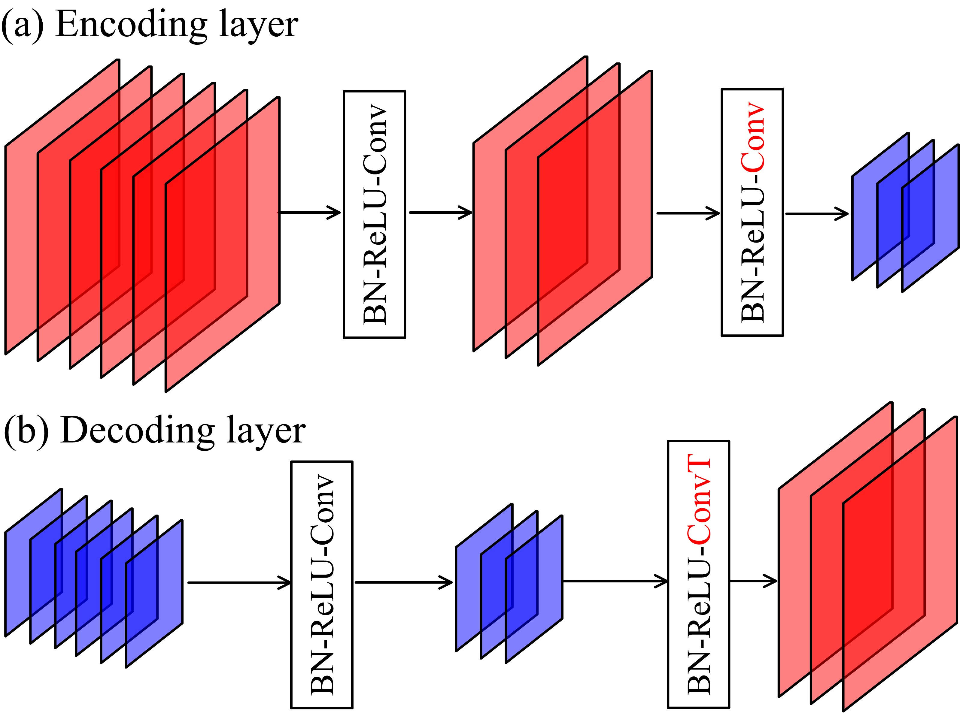
The output feature maps of a dense block are then fed into a transition layer. The transition layer, which is referred to as encoding layer in the encoder and as decoding layer in the decoder, is placed between two adjacent dense blocks to avoid feature maps explosion and to change the size of feature maps during the coarse-refine process. It halves the size of feature maps in the encoder (i.e., downsampling), while doubles the size in the decoder (i.e., upsampling). Both the encoding and decoding layers reduce the number of feature maps. An illustration of the encoding and decoding layers is given in Figure 2.
The network integrated architecture employed is depicted in Figure 3. The network is fully convolutional without any fully connected layers. Such architectures show better performance in pixel-wise classification compared to convolutional neural networks containing fully connected layers (Long et al., 2015). In the encoding path, the input image is fed into the first convolution layer. The extracted feature maps are then passed through an alternating cascade of dense blocks and encoding layers. The last encoding layer outputs high-level coarse feature maps, as shown with red boxes, which are subsequently fed into the decoder. The decoder is composed of an alternation of dense blocks and decoding layers, with the last decoding layer leading to the output images.

3.3 Deep Convolutional Encoder-Decoder Network for Approximating Time-Dependent Outputs
For dynamic systems, it is important to develop a surrogate that allows prediction of responses at arbitrary time instances. It is certainly computationally inefficient to construct independently surrogate models for outputs at all time instances of interest. A computationally attractive alternative is to treat the time as an input to the surrogate model and train the surrogate model with the outputs at only a limited number of time instances. Then the surrogate can potentially make predictions at time instances different from those used in the training data.
The surrogate for dynamic systems is
where is the model prediction at the input and time , and denotes all the network parameters. The training data is organized as , where denotes the simulation output, and is a re-index for . Also, and denote the total number of model runs and time instances when simulation data is stored in each run, respectively.
The time instance is broadcast as an extra feature map and concatenated with the latent feature maps (as shown with red boxes in Figure 3) extracted from the input since they independently impact the output .
3.4 Two-Stage Network Training Combining Regression and Segmentation Losses
Training the surrogate amounts to optimize the network parameters using training data with respect to certain loss function. The mean squared error (MSE) loss for the regression problem is defined as
| (15) |
where
| (16) |
Even though deep neural networks have a robust capacity to model complex output responses, accurately approximating the discontinuous saturation front in our multi-phase flow system remains a challenge. We address this problem by augmenting the original regression task with image segmentation for the output saturation field, which separates the area with saturation greater than zero from the area with zero saturation. The training data for segmentation is obtained by binarizing the saturation field. More specifically, we define the following indicator function pixel-wise:
| (17) |
where is the saturation. Given a saturation field, we can obtain a corresponding binary image with the response value at each pixel being or . Figure 4 shows an example of the saturation field and the corresponding binary image obtained by applying equation (17). The discontinuous saturation front in Figure 4a is clearly reflected by the boundary between and in Figure 4b.

The binary saturation field is treated as an extra output field of the forward model. Now the surrogate output becomes
| (18) |
The segmentation output is expected to capture the saturation front very well and thus carries this statistical strength to the original regression task that we are interested in.
We use the standard binary cross entropy (BCE) loss for this two-class segmentation task with training data
| (19) |
where
| (20) |
with being the number of pixels in the binary image.
In network training, the stochastic gradient descent (SGD) algorithm is used as the optimizer for parameter learning (Goodfellow et al., 2016). Let denote the loss function. In our model, the network is trained in a two-stage manner for each epoch:
(1) Train the network using the regularized MSE loss, i.e.,
| (21) |
where is the regularization coefficient, also called weight decay.
(2) Using the optimized parameter values in Step () as the starting point, optimize the network parameters based on a combination of the MSE and BCE losses, i.e.,
| (22) |
where is a weight balancing the two losses.
In the first stage, the network is trained aiming to accurately approximate the output fields as a traditional network will do in regression tasks. The second stage aims to refine the approximation around the discontinuous saturation front. As mentioned above, the segmentation loss is attributed to the mismatch in the regions around the discontinuous front, thus minimization of this loss can promote a further improvement in the approximation accuracy in those regions.
The SGD algorithms require computing the gradient of the loss with respect to . Taking the MSE loss as an example, we can write:
| (23) |
The computational cost of this operation may be very high when is large. In SGD, a minibatch strategy is used to reduce the computational burden, in which only a minibatch of samples uniformly drawn from the training set () are used (Goodfellow et al., 2016). Then the estimate of the gradient is given as
| (24) |
The SGD then follows the estimated gradient downhill:
| (25) |
where is the learning rate. Various SGD algorithms are available. The widely used Adam algorithm (Kingma and Ba, 2014) is adopted in this work.
The two-stage training strategy is summarized in Algorithm 1. Briefly speaking, in each epoch, all minibatches of the training sample set are utilized to optimize the network parameters. For each minibatch, the network parameters are updated twice: firstly updated using the gradient of (i.e., lines and in Algorithm 1); and then updated using the gradient of (i.e., lines and in Algorithm 1). The obtained values are then used as the starting point when using the next minibatch to update the parameters. In section 4, we will compare the performance of the network trained using the two-stage training strategy (i.e., Algorithm 1) with the network based solely on the traditional MSE loss (i.e., the stage one in Algorithm 1). This study will illustrate the effectiveness of the proposed two-stage training strategy in handling discontinuous outputs.
4 Numerical Experiments
4.1 Experiment Setting
4.1.1 GCS Multiphase Flow Model
To demonstrate the effectiveness and efficiency of our approach, we apply Algorithm 1 to a synthetic study of a geological carbon storage simulation. The synthetic model simulates the migration of CO2 within a 2-D domain. As shown in Figure 5, the m500 m aquifer domain lies in the plane with a grid size of m and a thickness of m. The initial pressure is assumed to be MPa with a constant temperature of ∘C and a salinity of by weight. The upper and lower boundaries are assumed to be with no-flux. The CO2 is injected into the 2-D aquifer at a constant rate of kg/s through injection wells located on the left boundary, while the right boundary is assumed to be fixed-state with a constant hydraulic pressure. The forward simulation is performed using TOUGH2/ECO2N (Pruess, 2005; Pruess et al., 1999) and the hydrogeologic properties used are summarized in Table 1. The van Genuchten-Mualem relative permeability function (Corey et al., 1954; Mualem, 1976; van Genuchten, 1980) and van Genuchten capillary pressure function (van Genuchten, 1980) are used. One single simulation with a simulation time of days takes about minutes on a Xeon E5-2660 GHz CPU.

| CO2 injection rate | kg/s |
| Reference permeability, | |
| Porosity (constant) | |
| Initial pressure | MPa |
| Temperature (isothermal) | ∘C |
| Salinity | |
| Relative permeability | |
| Irreducible water saturation | |
| Irreducible gas saturation | |
| Pore size distribution index | |
| Capillary pressure | |
| Irreducible water saturation | |
| Pore size distribution index | |
| Air entry pressure | Pa |
The objective of this benchmark problem is to quantify the uncertainty of the evolution of the pressure buildup and CO2 saturation in the cells over time. It is assumed that the uncertainty is only caused by the random heterogeneous permeability field (i.e., ). The application of the model to problems with multiple types of random input fields (i.e., ) is straightforward without requiring any modifications of the network structure. The pressure response in this example is always larger than the initial pressure, i.e., Pa, which is too large compared to the CO2 saturation. This may lead to an unstable neural network approximation, thus we rescale the pressure values as follows
| (26) |
In TOUGH2, the permeability heterogeneity is specified by assigning a permeability modifier to each cell , i.e.,
| (27) |
here is the reference permeability. The log-permeability field is assumed to be a Gaussian random field, thus the permeability modifier
| (28) |
Here, is the constant mean and an exponentiated quadratic covariance function is used, i.e.,
| (29) |
where s and s′ are two arbitrary locations in the domain, and and m are the variance and correlation length, respectively. Note that if this random field is parameterized using the Karhunen-Loève expansion (Zhang and Lu, 2004), expansion terms will be needed to preserve of the field variance. In the numerical examples, we directly treat the permeability at each spatial grid as an uncertain variable without using any dimensionality reduction methods, leading to an input dimension of (thus all pixel values of the permeability field are taken as uncorrelated).
One random realization of the permeability field is shown in Figure 5 and snapshots of the corresponding simulated pressure and CO2 saturation at time instances (, , and days) after CO2 injection are respectively shown in the first rows of Figure 8. It is observed that the pressure evolves relatively smoothly as it is generally insensitive to small-scale variability of the permeability (Kitanidis, 2015). In contrast, the permeability heterogeneity shows a significant influence on the migration of CO2. The saturation displays a complicated spatial variability (strongly nonlinear) and a sharp (discontinuous) front moving at varying speed. This strong nonlinearity and front discontinuity make the development of a surrogate model quite a challenging task.
4.1.2 Neural Network Design and Performance Evaluation Metrics
For the design of the network architecture, we follow the guidelines provided in Zhu and Zabaras (2018) and employ the most promising configuration which is illustrated in Figure 6 with more details on the parameter settings listed in Table 2. The number of initial feature maps after the first convolution layer is . The time enters the network as an extra feature map of the latent space after the last encoding layer. The network contains three dense blocks with , , and internal layers, and a constant growth rate . The convolution kernels are fixed to be for the first convolution layer, where the value for each parameter is denoted by the number to the right of the corresponding symbol, in the convolutional layers within the dense block, and for the first and second convolution layers, respectively, in both of the encoding and decoding layers, and for the transposed convolution layer in the last decoding layer.
We are interested in the spatiotemporal evolution of the pressure and saturation fields between and days after CO2 injection. Thus we collect the output pressure and CO2 saturation at time instances (, and days) to train the network. There are feature maps (i.e., the pressure field and the saturation field together with its corresponding binary representation image) in the output of the last layer (i.e., ). The sigmoid function is employed as the activation of the output layer to embed the prior knowledge that the saturation and rescaled pressure take values between and . The initial learning rate , weight decay , batch size , and binary segmentation loss weight . We also use a learning rate scheduler which drops times on plateau of the root mean squared error. The network is trained for epochs.

| Layers | Resolution | |
|---|---|---|
| Input | 1 | |
| Convolution | 48 | |
| Dense Block 1 | 144 | |
| Encoding Layer | 72 | |
| Dense Block 2 | 289 | |
| Decoding Layer 1 | 144 | |
| Dense Block 3 | 240 | |
| Decoding Layer 2 | 3 |
To evaluate the quality of the trained surrogate model, we consider two commonly used metrics, i.e., the coefficient of determination () and root mean squared error (RMSE). The metric is defined as
| (30) |
where is the number of samples, and are the TOUGH2 and deep network predicted outputs, respectively, and . The RMSE metric is written as
| (31) |
The metric is a normalized error enabling the comparison between different datasets, with the score closer to corresponding to better surrogate quality, while RMSE is a metric commonly used for monitoring the convergence of both the training and test errors during the training process.
4.2 Results
In this section, we assess the performance of our model in approximating the time-dependent multi-output of the geological carbon storage multiphase flow system in the case of high-dimensionality and response discontinuity. The approximation accuracy of the model is evaluated using randomly selected permeability test samples. To evaluate the significance of using the MSE-BCE loss in training our model, we also compare our results with those obtained from a network with the same architecture and training data but using only the MSE loss. Such a network has only two output images (the pressure and CO2 saturation fields). To distinguish between this network and our proposed network, we refer to them as the network with MSE loss and the network with MSE-BCE loss, respectively. The results obtained in uncertainty quantification tasks using our deep network based model are compared to those computed with vanilla MC.
4.2.1 Approximation Accuracy Assessment
To illustrate the convergence of the approximation error with respect to the training sample size, we generate four training sample sets with , , , and model evaluations. Figure 7a plots the RMSE decay with the number of epochs during the training process. The model is trained on a NVIDIA GeForce GTX Ti X GPU which requires about seconds for training epochs when the training sample size varies from to . Each sample includes system responses at time instances as discussed in section 4.1.2. It is observed that the RMSE starts to stabilize after epochs in all cases. The score for the test dataset for each surrogate with different training dataset sizes is shown in Figure 7b. The figure shows that with only training samples the model achieves a relatively high value of for a problem with stochastic input dimensions and in the presence of response discontinuity. When increasing the samples size to , the model achieves a value of .
Figure 7b clearly demonstrates that the model using the MSE-BCE loss achieves a higher value for a given dataset size than the network trained with the MSE loss. With training samples, the network with MSE loss only achieves a value of , much lower than that of the MSE-BCE loss based network (). As more training samples are available, the difference between the scores of the networks for the two loss functions decreases. The results indicate that the MSE-BCE loss training strategy substantially improves the model’s performance in approximating the multiphase flow GCS model especially when the training sample size is small.

The performance of our model in accurately approximating the multiphase flow model is further illustrated in Figures 8 and 9, which depict a comparison of the pressure and CO2 saturation fields at , and days predicted by TOUGH2 and our network model using and training samples, respectively. These predictions refer to the permeability realization shown in Figure 5 that is randomly selected from the test set. In both cases, the model as expected achieves higher approximation accuracy for the relatively smooth pressure field than for the strongly nonlinear and discontinuous saturation field. Even when using only training samples, the model is capable of capturing the nonlinear pressure field. It also reproduces the front discontinuity at all three time instances although with a higher approximation error. These are well-recognized challenges for other surrogate models (Liao and Zhang, 2013; Liao and Zhang, 2014; Xiu and Hesthaven, 2005). The relatively large approximation error of the model when using training samples is mainly caused by the large error in the approximation of the saturation front. When increasing the training sample size to , as shown in Figure 9, the model provides better characterization of the local nonlinear features as well as of the position of the saturation front.


Note that our model was trained with output data at time instances including and days but not days. It is clear that visually there is no significant difference between the approximation errors at time instances when training data were provided and other interpolated time instances in particular days. The model capability to accurately predict the time evolution of the output fields is further illustrated in Figure 10 which depicts the predicted pressure and CO2 saturation fields at time instances ranging every days from to days. We can see that the model provides good approximation at all time instances. The prediction errors at the time instances when training data were provided ( days) are similar to those in the remaining predictions at time instances. Thus by treating the time as an input and training with output data at only a limited number of time instances, the model is capable of approximating the time-dependent multi-output of the dynamic system efficiently.

Figure 11 shows the predictions of the MSE loss based model with training samples for the same output fields shown in Figure 8. Comparing with Figure 8, it can be seen that visually there is no significant difference in the pressure and saturation fields approximation errors between the two models except near the saturation front. However, it is observed that the MSE-BCE loss based model provides better characterizations for the saturation front positions than the MSE loss based model. This is demonstrated in Figure 12 which compares the binary images obtained from binarizing the saturation fields in Figures 8 and 11 using equation (17). The pixels with value reflect the distribution of CO2 plume and the edges between pixels with values and correspond to the positions of the saturation front. It is observed that the model with the MSE-BCE loss function provides more accurate prediction for the positions of the saturation front. For surrogate modeling of the saturation field, underestimating (overestimating) the position of the discontinuous saturation front will lead to an underestimation (overestimation) of the saturation in the regions between the predicted and actual fronts, resulting in large approximation errors.


Figure 13 shows the predictions of the MSE-BCE loss function deep network model trained with four different datasets for the binary image at days shown in the upper right of Figure 12. For the four cases, the approximations for the binary image are rather accurate except near the saturation front. The BCE loss is mostly induced by the approximation errors in regions around the saturation front and considering it in addition to the standard MSE loss promotes a more accurate approximation of the discontinuous front.

In the above experiments, the BCE loss weight was chosen as . This weight decides the influence of the BCE loss on the hybrid loss in equation (22). It is understandable that a lager will promote a better approximation of the discontinuous saturation front. However, our objective in surrogate modeling of multiphase flow models is not only to accurately characterize the discontinuous saturation front, but more importantly to provide globally accurate approximation for the entire output fields. The value of should be chosen carefully. To investigate the influence of on the performance of our method, we test five different values of ranging from to . The corresponding results are shown in Figure 14, which depicts the scores and RMSEs of networks with different values evaluated on test samples. It is observed that among the five surrogates the one with performs best, and that the performance decreases when increasing or reducing the weight. We further analyze the decay of the values of the MSE loss and weighted BCE loss during the training process. As shown in Figure 15, the network with has similar MSE and weighted BEC loss values during the training process, thus putting similar weights on global regression of the output fields and approximation of the saturation front. In contrast, the networks with and focus more on global regression (larger MSE loss than weighted BCE loss) and local refinement (larger weighted BCE loss than MSE loss), respectively. According to these results, a value is recommended that equally weighs the MSE and BCE losses.


Recall that we use a dense fully convolutional encoder-decoder network architecture in our method to transform the surrogate modeling task to an image-to-image regression problem. The above results indicate that, first of all, the method shares the good property of CNNs in image processing, making it robust in handling high-dimensional input and output fields (images). Secondly, the use of deep neural networks provides high flexibility and robust capability for surrogate modeling of strongly nonlinear and discontinuous responses. In addition, it was shown that treating time as an additional input to the network, the model can efficiently provide prediction of time-dependent outputs of dynamic systems at any time instance. Finally, the densely connected convolutional network architecture (i.e., dense block) was shown to substantially enhance the exploitation of local information of data and improve the feature flow through the network, which has also been illustrated in Huang et al. (2017) and Zhu and Zabaras (2018). As a result, the developed model was able to provide relatively good approximation with limited training samples effectively resolving the three challenges associated with surrogate modeling of multi-phase flow models discussed in section 1.

4.2.2 Uncertainty modeling
In this section, we test our model’s effectiveness and efficiency in addressing UQ tasks for the GCS model. The MSE-BCE loss based network model is trained with samples. Uncertainty quantification is performed using MC approximations. Monte Carlo sampling is conducted on the cheap-to-evaluate surrogate instead of the computationally intensive GCS model. This means that the deep network is used as a full replacement of the GCS model and thus no extra model evaluations are required. The computational cost is mainly from the evaluation of the training samples needed for the surrogate construction. We randomly generate MC realizations by direct GCS model runs to compute the reference statistics. We use the deep network and TOUGH2 to predict the system response for the same input realizations when performing UQ. In this way, the possible inaccuracy in the UQ solution will only be caused by the approximation error of the surrogate model.

Figures 16 and 17 illustrate the mean and variance of the pressure and CO2 saturation fields at , and days, respectively. As CO2 is injected from the left boundary with an equal injection rate for all cells, the isolines of mean fields are approximately parallel to the -axis (Figure 16) and as expected much smoother than those corresponding to a single permeability realization. However, the variance of the CO2 saturation around the front is relatively large with large gradients because of the presence of the discontinuity. It can be seen that both the mean and variance fields predicted by the model including those at time instances (e.g., days) where no training data were provided are very close to the reference solutions.

Next, we look at the PDFs of the pressure and CO2 saturation. Figures 18 and 19 show the PDFs of pressure and CO2 saturation at times instances at locations ( m, m) and ( m, m), respectively. We also plot the estimated PDFs from MC sampling using the same number (i.e., ) of model executions as we used in the network training. This would allow us to compare the accuracy of these two estimators that have the same cost in terms of needed data versus the reference MC solution obtained with samples. We observe that, for the pressure, the PDFs obtained from the surrogate model at all time instances are almost identical to the reference solution. In addition, the bimodal nature of the PDFs of CO2 saturation is successfully captured. The slight mismatch is mainly caused by the error in predicting the location of the discontinuity front. Again, the accuracy of the PDFs at the time instance where no training data were provided (e.g., days) is visually the same to that at the training time instances (i.e., and days). Note that to obtain an almost identical result to the reference solution, the deep network-based MC simulation only uses model runs for surrogate construction. On the other hand, with the same model runs, the traditional MC obtains the estimated PDFs that show a large approximation error (the blue dot dash lines) especially for the bimodal PDFs of saturation.

The model’s performance in capturing the bimodal PDFs of saturation is further illustrated in Figures 20 and 21, which depict the PDFs of CO2 saturation at four locations along the -axis at the time instances and days, respectively. It is observed that the model accurately reproduces the bimodal PDFs at both time instances. By treating the time as an additional input and training the network with the outputs at a limited number of time instances, the model can make predictions at arbitrary time instances, enabling the characterization of dynamic systems. The results indicate that the proposed method can efficiently provide accurate solutions of UQ for the dynamic multiphase flow GCS model in the case of high-dimensionality and response discontinuity.


5 Conclusions
Surrogate methods are used widely to alleviate the large computational burden associated with uncertainty quantification. However, there are situations that hinder their application to transient multi-phase flow problems due to the high-dimensionality and response discontinuity. In this study, a new deep convolutional neural network approach is proposed for such dynamic problems using an encoder-decoder network architecture that transformed the surrogate modeling problem to an image-to-image regression problem. The encoder is used to extract the underlying features from the high-dimensional input images (fields) which are subsequently used by the decoder to reconstruct the output images (responses). In order to address the need for big data in training deep learning models, a dense fully convolutional neural network (CNN) structure is employed. It is well-suitable for image processing since it substantially strengthens the information flow through the network. The deep network structure based on CNNs implicitly reduces the input dimensionality through a series of inherent nonlinear projections of the input into high-level coarse feature maps while providing a robust capability to handle complex output responses.
In addition, a training strategy combining a regression loss and a segmentation loss is introduced in order to better approximate the discontinuous saturation field. The segmentation loss is mostly induced by the mismatch in regions around the discontinuous saturation front, thus facilitating a better approximation of the discontinuity. To address the dynamic nature of the problem, time is treated as an extra input to the network that is trained using model outputs at a limited number of time instances.
The performance of the method developed is demonstrated using a geological carbon storage process-based multiphase flow model with uncertain input parameters. The results indicate that the image-to-image regression strategy is robust in handling problems with high-dimensional input and output fields with discontinuous response. The method successfully reproduces the saturation discontinuity and provides accurate approximations of the pressure and saturation fields. Moreover, it is able to characterize the time-dependent multi-output of the dynamic system at arbitrary time instances. The application of the method in addressing uncertainty quantification tasks for the GCS model showed that the deep network based surrogate model can achieve comparably accurate results to those obtained with traditional Monte Carlo sampling but at a much higher efficiency requiring significantly fewer GCS model runs.
It is worth noting that the ability of the deep network approach to model the dynamic behavior of complex systems is not only useful for uncertainty quantification problems but also holds promise for experimental design tasks or for the solution of inverse problems (Zhang et al., 2015; Zhang et al., 2016, e.g.,). The model presented can be extended to multiple input fields (e.g. permeability and porosity) without any modifications of the network architecture. Its potential use as a surrogate model for many complex systems beyond groundwater multi-phase flows remains to be explored.
Acknowledgements.
S.M. acknowledges the China Scholarship Council for financially supporting his study at the Center for Informatics and Computational Science (CICS) at the University of Notre Dame. N.Z. and Y.Z. acknowledge support from the University of Notre Dame and CICS. The work of S.M., X.S. and J.W. was supported by the National Natural Science Foundation of China (No. U and ). The Python codes and data used will be made available at https://github.com/cics-nd/dcedn-gcs upon publication of this manuscript. The data used can be reproduced using TOUGH2 (http://esd1.lbl.gov/research/projects/tough/) and the needed scripts are available upon request from the corresponding authors.References
- Al-Rfou et al. (2016) Al-Rfou, R., G. Alain, A. Almahairi, C. Angermueller, D. Bahdanau, N. Ballas, F. Bastien, J. Bayer, A. Belikov, A. Belopolsky, et al. (2016), Theano: A python framework for fast computation of mathematical expressions, arXiv preprint arXiv:1605.02688, 472, 473.
- Asher et al. (2015) Asher, M. J., B. F. W. Croke, A. J. Jakeman, and L. J. M. Peeters (2015), A review of surrogate models and their application to groundwater modeling, Water Resources Research, 51(8), 5957–5973, 10.1002/2015WR016967.
- Badrinarayanan et al. (2017) Badrinarayanan, V., A. Kendall, and R. Cipolla (2017), Segnet: A deep convolutional encoder-decoder architecture for image segmentation, IEEE transactions on pattern analysis and machine intelligence, 39(12), 2481–2495.
- Ballio and Guadagnini (2004) Ballio, F., and A. Guadagnini (2004), Convergence assessment of numerical monte carlo simulations in groundwater hydrology, Water Resources Research, 40(4), n/a–n/a, 10.1029/2003WR002876, w04603.
- Benson and Orr (2008) Benson, S. M., and F. M. Orr (2008), Carbon dioxide capture and storage, MRS Bulletin, 33(4), 303–305, 10.1557/mrs2008.63.
- Birkholzer et al. (2015) Birkholzer, J. T., C. M. Oldenburg, and Q. Zhou (2015), Co2 migration and pressure evolution in deep saline aquifers, International Journal of Greenhouse Gas Control, 40, 203 – 220, https://doi.org/10.1016/j.ijggc.2015.03.022, special Issue commemorating the 10th year anniversary of the publication of the Intergovernmental Panel on Climate Change Special Report on CO2 Capture and Storage.
- Celia et al. (2015) Celia, M. A., S. Bachu, J. M. Nordbotten, and K. W. Bandilla (2015), Status of co2 storage in deep saline aquifers with emphasis on modeling approaches and practical simulations, Water Resources Research, 51(9), 6846–6892, 10.1002/2015WR017609.
- Chan and Elsheikh (2017) Chan, S., and A. H. Elsheikh (2017), Parametrization and generation of geological models with generative adversarial networks, arXiv preprint arXiv:1708.01810.
- Chan and Elsheikh (2018) Chan, S., and A. H. Elsheikh (2018), A machine learning approach for efficient uncertainty quantification using multiscale methods, Journal of Computational Physics, 354, 493 – 511, https://doi.org/10.1016/j.jcp.2017.10.034.
- Cihan et al. (2013) Cihan, A., J. T. Birkholzer, and Q. Zhou (2013), Pressure buildup and brine migration during co2 storage in multilayered aquifers, Groundwater, 51(2), 252–267, 10.1111/j.1745-6584.2012.00972.x.
- Corey et al. (1954) Corey, A. T., et al. (1954), The interrelation between gas and oil relative permeabilities, Producers monthly, 19(1), 38–41.
- Crevilléén-García et al. (2017) Crevilléén-García, D., R. Wilkinson, A. Shah, and H. Power (2017), Gaussian process modelling for uncertainty quantification in convectively-enhanced dissolution processes in porous media, Advances in Water Resources, 99, 1 – 14, https://doi.org/10.1016/j.advwatres.2016.11.006.
- Dumoulin and Visin (2016) Dumoulin, V., and F. Visin (2016), A guide to convolution arithmetic for deep learning, arXiv preprint arXiv:1603.07285.
- Ganapathysubramanian and Zabaras (2007) Ganapathysubramanian, B., and N. Zabaras (2007), Sparse grid collocation schemes for stochastic natural convection problems, Journal of Computational Physics, 225(1), 652 – 685, https://doi.org/10.1016/j.jcp.2006.12.014.
- Goodfellow et al. (2016) Goodfellow, I., Y. Bengio, and A. Courville (2016), Deep Learning, MIT Press.
- Gu et al. (2018) Gu, J., Z. Wang, J. Kuen, L. Ma, A. Shahroudy, B. Shuai, T. Liu, X. Wang, G. Wang, J. Cai, and T. Chen (2018), Recent advances in convolutional neural networks, Pattern Recognition, 77, 354 – 377, https://doi.org/10.1016/j.patcog.2017.10.013.
- He et al. (2016) He, K., X. Zhang, S. Ren, and J. Sun (2016), Deep residual learning for image recognition, in Proceedings of the IEEE conference on computer vision and pattern recognition, pp. 770–778.
- Hornik et al. (1989) Hornik, K., M. Stinchcombe, and H. White (1989), Multilayer feedforward networks are universal approximators, Neural Networks, 2(5), 359 – 366, https://doi.org/10.1016/0893-6080(89)90020-8.
- Huang et al. (2017) Huang, G., Z. Liu, K. Q. Weinberger, and L. van der Maaten (2017), Densely connected convolutional networks, in Proceedings of the IEEE conference on computer vision and pattern recognition, vol. 1, p. 3.
- Ioffe and Szegedy (2015) Ioffe, S., and C. Szegedy (2015), Batch normalization: Accelerating deep network training by reducing internal covariate shift, arXiv preprint arXiv:1502.03167.
- Kingma and Ba (2014) Kingma, D. P., and J. Ba (2014), Adam: A method for stochastic optimization, CoRR, abs/1412.6980.
- Kitanidis (2015) Kitanidis, P. K. (2015), Persistent questions of heterogeneity, uncertainty, and scale in subsurface flow and transport, Water Resources Research, 51(8), 5888–5904, 10.1002/2015WR017639.
- Laloy et al. (2013) Laloy, E., B. Rogiers, J. A. Vrugt, D. Mallants, and D. Jacques (2013), Efficient posterior exploration of a high-dimensional groundwater model from two-stage markov chain monte carlo simulation and polynomial chaos expansion, Water Resources Research, 49(5), 2664–2682, 10.1002/wrcr.20226.
- Laloy et al. (2017) Laloy, E., R. Hérault, J. Lee, D. Jacques, and N. Linde (2017), Inversion using a new low-dimensional representation of complex binary geological media based on a deep neural network, Advances in Water Resources, 110, 387 – 405, https://doi.org/10.1016/j.advwatres.2017.09.029.
- Laloy et al. (2018) Laloy, E., R. Hérault, D. Jacques, and N. Linde (2018), Training-image based geostatistical inversion using a spatial generative adversarial neural network, Water Resources Research, pp. n/a–n/a, 10.1002/2017WR022148.
- Li and Zhang (2007) Li, H., and D. Zhang (2007), Probabilistic collocation method for flow in porous media: Comparisons with other stochastic methods, Water Resources Research, 43(9), n/a–n/a, 10.1029/2006WR005673, w09409.
- Li et al. (2009) Li, W., Z. Lu, and D. Zhang (2009), Stochastic analysis of unsaturated flow with probabilistic collocation method, Water Resources Research, 45(8), n/a–n/a, 10.1029/2008WR007530, w08425.
- Li et al. (2017) Li, Y. J., A. Kokkinaki, E. F. Darve, and P. K. Kitanidis (2017), Smoothing-based compressed state kalman filter for joint state-parameter estimation: Applications in reservoir characterization and co2 storage monitoring, Water Resources Research, 53(8), 7190–7207, 10.1002/2016WR020168.
- Liao and Zhang (2013) Liao, Q., and D. Zhang (2013), Probabilistic collocation method for strongly nonlinear problems: 1. transform by location, Water Resources Research, 49(12), 7911–7928, 10.1002/2013WR014055.
- Liao and Zhang (2014) Liao, Q., and D. Zhang (2014), Probabilistic collocation method for strongly nonlinear problems: 2. transform by displacement, Water Resources Research, 50(11), 8736–8759, 10.1002/2014WR016238.
- Liao and Zhang (2016) Liao, Q., and D. Zhang (2016), Probabilistic collocation method for strongly nonlinear problems: 3. transform by time, Water Resources Research, 52(3), 2366–2375, 10.1002/2015WR017724.
- Liao et al. (2017) Liao, Q., D. Zhang, and H. Tchelepi (2017), A two-stage adaptive stochastic collocation method on nested sparse grids for multiphase flow in randomly heterogeneous porous media, Journal of Computational Physics, 330, 828 – 845, https://doi.org/10.1016/j.jcp.2016.10.061.
- Lin and Tartakovsky (2009) Lin, G., and A. Tartakovsky (2009), An efficient, high-order probabilistic collocation method on sparse grids for three-dimensional flow and solute transport in randomly heterogeneous porous media, Advances in Water Resources, 32(5), 712 – 722, https://doi.org/10.1016/j.advwatres.2008.09.003.
- Long et al. (2015) Long, J., E. Shelhamer, and T. Darrell (2015), Fully convolutional networks for semantic segmentation, in Proceedings of the IEEE conference on computer vision and pattern recognition, pp. 3431–3440.
- Lu et al. (2016) Lu, D., G. Zhang, C. Webster, and C. Barbier (2016), An improved multilevel monte carlo method for estimating probability distribution functions in stochastic oil reservoir simulations, Water Resources Research, 52(12), 9642–9660, 10.1002/2016WR019475.
- Lu et al. (2018) Lu, D., D. Ricciuto, and K. Evans (2018), An efficient bayesian data-worth analysis using a multilevel monte carlo method, Advances in Water Resources, 113, 223–235, https://doi.org/10.1016/j.advwatres.2018.01.024.
- Ma and Zabaras (2009) Ma, X., and N. Zabaras (2009), An adaptive hierarchical sparse grid collocation algorithm for the solution of stochastic differential equations, Journal of Computational Physics, 228(8), 3084 – 3113, https://doi.org/10.1016/j.jcp.2009.01.006.
- Ma and Zabaras (2010) Ma, X., and N. Zabaras (2010), An adaptive high-dimensional stochastic model representation technique for the solution of stochastic partial differential equations, Journal of Computational Physics, 229(10), 3884 – 3915, https://doi.org/10.1016/j.jcp.2010.01.033.
- Meng and Li (2017) Meng, J., and H. Li (2017), An efficient stochastic approach for flow in porous media via sparse polynomial chaos expansion constructed by feature selection, Advances in Water Resources, 105, 13 – 28, https://doi.org/10.1016/j.advwatres.2017.04.019.
- Mo et al. (2017) Mo, S., D. Lu, X. Shi, G. Zhang, M. Ye, J. Wu, and J. Wu (2017), A taylor expansion-based adaptive design strategy for global surrogate modeling with applications in groundwater modeling, Water Resources Research, 53(12), 10,802–10,823, 10.1002/2017WR021622.
- Mualem (1976) Mualem, Y. (1976), A new model for predicting the hydraulic conductivity of unsaturated porous media, Water Resources Research, 12(3), 513–522, 10.1029/WR012i003p00513.
- Müller et al. (2011) Müller, F., P. Jenny, and D. W. Meyer (2011), Probabilistic collocation and lagrangian sampling for advective tracer transport in randomly heterogeneous porous media, Advances in Water Resources, 34(12), 1527 – 1538, https://doi.org/10.1016/j.advwatres.2011.09.005.
- Pruess (2005) Pruess, K. (2005), ECO2N: A TOUGH2 fluid property module for mixtures of water, NaCl, and CO2, Lawrence Berkeley National Laboratory Berkeley, Berkeley, CA, USA.
- Pruess et al. (1999) Pruess, K., C. Oldenburg, and G. Moridis (1999), Tough2 user’s guide version 2, Tech. rep., Lawrence Berkeley National Laboratory, Berkeley, CA, USA.
- Rasmussen and Williams (2006) Rasmussen, C. E., and C. K. I. Williams (2006), Gaussian Processes for Machine Learning, MIT Press.
- Razavi et al. (2012) Razavi, S., B. A. Tolson, and D. H. Burn (2012), Review of surrogate modeling in water resources, Water Resources Research, 48(7), n/a–n/a, 10.1029/2011WR011527, w07401.
- Tian et al. (2017) Tian, L., R. Wilkinson, Z. Yang, H. Power, F. Fagerlund, and A. Niemi (2017), Gaussian process emulators for quantifying uncertainty in co2 spreading predictions in heterogeneous media, Computers & Geosciences, 105, 113 – 119, https://doi.org/10.1016/j.cageo.2017.04.006.
- Tripathy and Bilionis (2018) Tripathy, R., and I. Bilionis (2018), Deep uq: Learning deep neural network surrogate models for high dimensional uncertainty quantification, arXiv preprint arXiv:1802.00850.
- van Genuchten (1980) van Genuchten, M. T. (1980), A closed-form equation for predicting the hydraulic conductivity of unsaturated soils 1, Soil science society of America journal, 44(5), 892–898.
- Xiu and Hesthaven (2005) Xiu, D., and J. S. Hesthaven (2005), High-order collocation methods for differential equations with random inputs, SIAM Journal on Scientific Computing, 27(3), 1118–1139, 10.1137/040615201.
- Xiu and Karniadakis (2002) Xiu, D., and G. E. Karniadakis (2002), The wiener–askey polynomial chaos for stochastic differential equations, SIAM Journal on Scientific Computing, 24(2), 619–644, 10.1137/S1064827501387826.
- Zhang and Lu (2004) Zhang, D., and Z. Lu (2004), An efficient, high-order perturbation approach for flow in random porous media via karhunen-loève and polynomial expansions, Journal of Computational Physics, 194(2), 773 – 794, https://doi.org/10.1016/j.jcp.2003.09.015.
- Zhang et al. (2013) Zhang, G., D. Lu, M. Ye, M. Gunzburger, and C. Webster (2013), An adaptive sparse-grid high-order stochastic collocation method for bayesian inference in groundwater reactive transport modeling, Water Resources Research, 49(10), 6871–6892, 10.1002/wrcr.20467.
- Zhang et al. (2015) Zhang, J., L. Zeng, C. Chen, D. Chen, and L. Wu (2015), Efficient bayesian experimental design for contaminant source identification, Water Resources Research, 51(1), 576–598, 10.1002/2014WR015740.
- Zhang et al. (2016) Zhang, J., W. Li, L. Zeng, and L. Wu (2016), An adaptive gaussian process-based method for efficient bayesian experimental design in groundwater contaminant source identification problems, Water Resources Research, 52(8), 5971–5984, 10.1002/2016WR018598.
- Zhu and Zabaras (2018) Zhu, Y., and N. Zabaras (2018), Bayesian deep convolutional encoder-decoder networks for surrogate modeling and uncertainty quantification, Journal of Computational Physics, 366, 415–447, https://doi.org/10.1016/j.jcp.2018.04.018.