Waveform to Single Sinusoid Regression to Estimate the F0 Contour from Noisy Speech Using Recurrent Deep Neural Networks
Abstract
The fundamental frequency () represents pitch in speech that determines prosodic characteristics of speech and is needed in various tasks for speech analysis and synthesis. Despite decades of research on this topic, estimation at low signal-to-noise ratios (SNRs) in unexpected noise conditions remains difficult. This work proposes a new approach to noise robust estimation using a recurrent neural network (RNN) trained in a supervised manner. Recent studies employ deep neural networks (DNNs) for tracking as a frame-by-frame classification task into quantised frequency states but we propose waveform-to-sinusoid regression instead to achieve both noise robustness and accurate estimation with increased frequency resolution.
Experimental results with PTDB-TUG corpus contaminated by additive noise (NOISEX-92) demonstrate that the proposed method improves gross pitch error (GPE) rate and fine pitch error (FPE) by more than 35 % at SNRs between -10 dB and +10 dB compared with well-known noise robust tracker, PEFAC. Furthermore, the proposed method also outperforms state-of-the-art DNN-based approaches by more than 15 % in terms of both FPE and GPE rate over the preceding SNR range.
Akihiro Kato, Tomi Kinnunen
University of Eastern Finland
akihiro.kato@uef.fi, tomi.kinnunen@uef.fi
Index Terms: estimation, pitch estimation, prosody analysis, voice activity detection, recurrent neural networks
1 Introduction
Fundamental frequency () is the lowest frequency in a quasi-periodic signal. It represents pitch in speech that determines prosodic characteristics of speech. Therefore, is one of the key features of speech and estimation is vital for many applications, e.g. voice conversion [1], speaker and language identification [2, 3], prosody analysis [4], speech coding [5], speech synthesis [6] and speech enhancement [7, 8].
Over the past decades, various approaches to estimation have been proposed. Specifically, robust algorithm for pitch tracking (RAPT) [9] and YIN [10] that track from time-domain signals have been widely used in many applications showing high accuracy [11]. These methods, however, do not attain satisfactory performance under noisy conditions [12]. Thus, several more noise robust methods have been proposed. For instance, pitch estimation filter with amplitude compression (PEFAC) [13] tends to outperform both RAPT and YIN in terms of noise robustness. It analyses noisy signals in the log-frequency domain with a matched filter and normalisation with the universal long-term average speech spectrum. Nonetheless, it remains challenging to obtain satisfactory estimates of at low signal-to-noise ratios (SNRs) such as 0 dB and below.
In addition to such real-time digital signal processing (DSP) methods, various machine learning approaches using Gaussian mixture models (GMMs) and hidden Markov models (HMMs) [14, 15], for example, have been developed for noise robust estimation. Furthermore, recent research has successfully applied deep neural networks (DNNs) and their variants, e.g. convolutional neural networks (CNNs) and recurrent neural networks (RNNs), to improve estimation in severe noise conditions [6, 16, 17]. DNNs derive discriminative models to represent arbitrarily complex mapping functions as long as they comprise enough number of units in their hidden layers. Consequently, they enable statistical models to deal with higher dimensional input features having stronger correlation than the preceding approaches.
Recently, another technical trend in acoustic modelling has emerged since a remarkable achievement of WaveNet [18], which analyses time-domain waveforms directly instead of extracting spectral or cepstral features from speech. This contributed to not only advancement in speech synthesis but also end-to-end modelling for various speech applications that do not require traditional Fourier analysis [18]. Direct analysis of waveforms is also beneficial for denoising of speech that usually combines noisy phase spectra with enhanced magnitude spectra to reconstruct clean speech [19].
In fact, the latest research has applied direct time-domain waveform analysis to estimation with DNN-based [20] and CNN-based [21] approaches showing improved noise robustness over both the conventional real-time signal processing and the recent DNN-based spectral analysis. These state-of-the-art time-domain estimators, however, still have a problem to be solved: they employ DNNs or CNNs to form a frame-by-frame classification model to decide a state corresponding to a quantised frequency. Even if it is convenient to treat tracking as a classification task in the same manner as alignment of senones in speech recognition, the resultant estimates of contours have a limited frequency resolution determined by the number of quantised frequency states. This is a potential draw-back in terms of estimation accuracy of .
This work is an extension of our recent preliminary study [22]. In that study, we have successfully employed an RNN regression model, which maps spectral sequence directly onto values, to tackle the disadvantage in existing classification approaches mentioned above. In relation to that preliminary study, the present paper represents the following four major changes. First, we employ direct waveform inputs instead of spectral sequence. Second, we propose a novel encoding method of the information using a simple sinusoid oscillated with the ground truth value of . This encoding enables our model to map raw speech waveforms to raw sinusoids without requirement of neither pre-processing nor post-processing. Next, we amend our experiments with very recent competitive methods which are also based on waveform input schemes [20, 21]. Finally, we augmented noise conditions for the experiments in order to examine noise robustness against more various noise types. Consequently, a known noise condition is increased from consisting of six noise types to eight types while an unknown noise condition is augmented from two types to four types.
2 Methodology
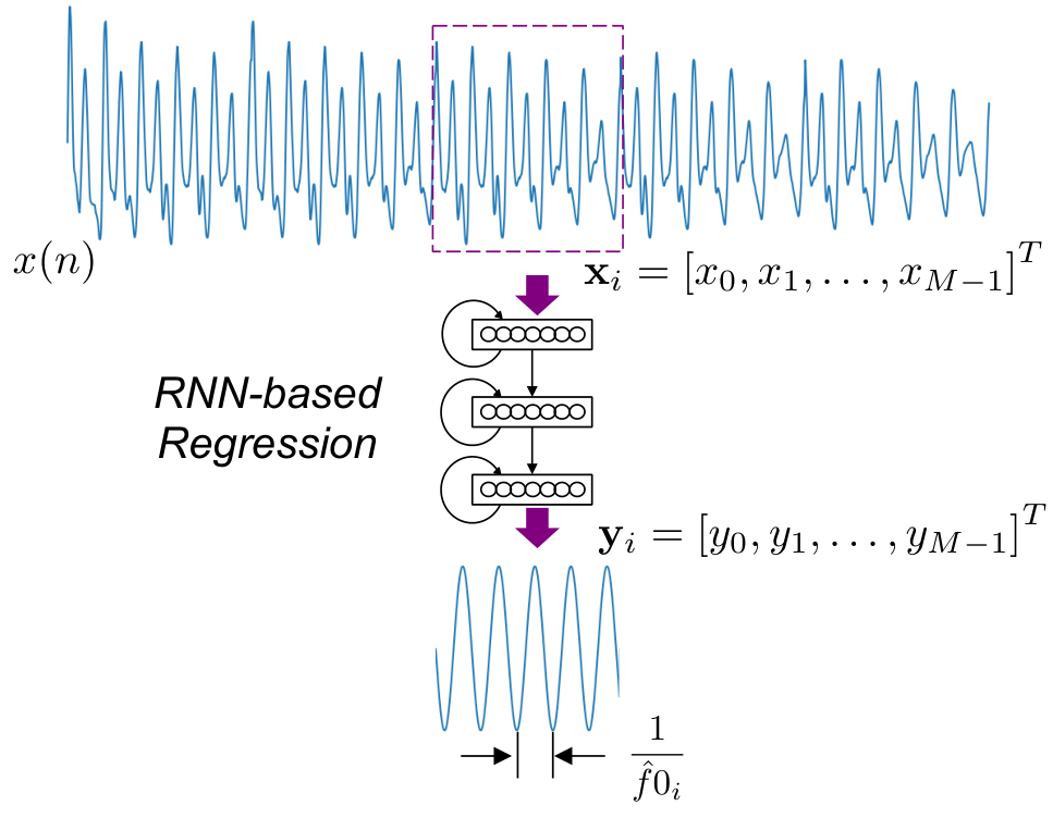
In the proposed method of estimation, discrete time-domain speech waveform, , is used as an input to an RNN. For voiced input speech, the posteriors of the RNN are mapped onto a single sinusoid oscillated with of the input waveform as a regression task. For unvoiced and no voice inputs, the RNN performs an identity mapping. The value is then explicitly inferred from the resultant single sinusoid using its autocorrelation. Figure 1 illustrates the proposed framework.
2.1 Waveform-to-sinusoid regression using an RNN
is first divided into frames, , , …, ,
| (1) |
where denotes the number of samples in a frame.
Units in RNN layers have connections from their outputs back to their own inputs in addition to the feedforward connections. Therefore, an RNN layer receives its own output at the previous time sequence as well as the current time sequence input from the previous layer. This behaviour of RNN layers, interpreted as memory cells [23], is well-suited to analyse temporal dynamics of speech. Thus, at the -th frame, , is analysed with neighbouring frames, i.e. to , sequence-by-sequence.
Since the RNN-based discriminative model in the proposed method takes a form of sequence-to-sequence structure, output of RNN layer, , at time sequence, , , is derived as follows with respect to input instance, .
| (2) | |||||
| (3) | |||||
| (4) |
where represents an activation function and is the weight matrix from the output of layer to the input of layer (feedforward) while denotes the weight matrix from the output of layer to the input of layer (feedback). Here, and are represented as
where is the number of units (excluding the bias unit) in the -th layer. Furthermore, is the feedforward weight between unit, , in the ()-th layer and unit, , in the -th layer while is the feedback weight between the output of unit, , and the input of unit, , in the -th layer.
In order to achieve the RNN-based regression to a single sinusoid, the output layer is activated by the identity function unlike classification model applying the softmax function for the activation. Consequently, posteriors of the RNN at the -th frame (i.e. ), , is derived as
| (15) | |||||
| (16) |
where and denote the identity function and the number of RNN layers respectively.
2.2 Model training and F0 estimation
In the offline training process, and are optimised in advance by supervised learning. During voiced speech periods, training is achieved by minimising the mean square error (MSE) between and its target sinusoid. The sinusoid is oscillated with and which are the ground truth of at frame, , and the phase to maximise the cross-correlation between and . Here, is the sampling frequency and , as illustrated in Figure 2.
For unvoiced and no voice periods, the target of supervised learning is set to the input waveform itself, i.e. identity mapping. The weight optimisation during this training is accomplished with mini-batch gradient descent with the backpropagation algorithm [24].
Finally, estimate of at the -th frame including voiced, unvoiced and no voice frames, , is inferred from by maximising its autocorrelation. Since unvoiced and no voice frames are transformed with identity mapping, those frames can be effectively detected if the maximum of cross correlation between and is lower than threshold, . In other words, voiced frames are easily distinguished if the shape of is close to a sinusoid, otherwise the frame is unvoiced or no voice. is empirically selected as 0.15 by preliminary cross-validation test. Figure 3 (a) demonstrates the relation between input voiced waveform, , and sinusoid obtained by the proposed RNN model, , at different SNRs in white noise. (b) plots their magnitude spectra to illustrate how is suitable for analysis compared with .
3 Experiments
We examine both accuracy and noise robustness of the proposed methods and compare them with RAPT [9], YIN [10], PEFAC [13] and state-of-the-art DNN-based classification approaches: DNN-CLS(S) [16], DNN-CLS(W) [20] and CREPE [21]. DNN-CLS(S) is based on a DNN classification model from spectral features to quantised frequency states whereas DNN-CLS(W) uses a DNN classification model from waveforms to quantised frequency states. CREPE is an tracker targeting at music signals using a CNN-based classification model from waveforms to quantised frequency states.
Performance of these trackers is evaluated in terms of two standard metrics: gross pitch error (GPE) rate and fine pitch error (FPE) [27]. GPE frames represent voiced frames in which the error between the estimated pitch period () and the ground truth () is more than 10 samples, i.e. 0.625 ms. FPE frames, in turn, are voiced frames excluding GPE frames. The mean of FPEs, , represents the bias in estimation whereas the standard deviation of FPEs, , measures the accuracy of estimation [27].
3.1 Datasets (PTDB-TUG corpus + NOISEX-92)
The experiments use speech from pitch tracking database from Graz University of Technology (PTDB-TUG) [11]. The training set consists of 3200 utterances spoken by 16 speakers (8 males, 8 females), i.e. 200 utterances each. The cross-validation (CV) set comprises other 576 utterances spoken by the same 16 speakers, 36 utterances per each. For the test set, 944 utterances spoken by 4 speakers (2 males, 2 females) who are not in the training and CV sets (unknown speakers), i.e. 236 utterances each, are contained in order to set the test condition as speaker independent (SI).
Speech in each dataset is sampled at 16kHz and the sampled signals in the training and CV sets are contaminated with eight types of additive noise at five levels of SNR, -10, -5, 0, +5 and +10 dB. The noise types are referred to as Babble, Destroyerops, F16, Factory2, Leopard, M109, Machinegun and White in NOISEX-92 [28]. The test set is contaminated with other four types of additive noise including Destroyerengine, Factory1, Pink and Volvo in addition to the preceding eight types at the same SNRs as the training and CV sets. The former four types make an unknown noise condition while the latter eight types give a known noise condition. Consequently, the training set amounts 131,200 utterances (15,252 min), i.e. 3,200 (8 noise 5 level + 1 clean), and the CV set becomes 23,616 utterances (2,542 min) while the test set amounts 57,584 utterances (6,344 min), i.e. 944 (12 noise 5 level + 1 clean), in total.
PTDB-TUG contains ground truth contours of each utterance obtained from laryngograph signals recorded in a clean condition to which a Kaiser filter and RAPT were applied. These are used in the following experiments as the ground truth.
3.2 Training and test settings
The speech signals in the datasets are framed into 25 ms frames at 5 ms intervals. The first 400 frames and the last 200 frames of each utterance are then removed to reduce non-speech frames.
The hyperparameters of the proposed method are empirically selected by preliminary cross-validation test. The number of hidden layers (LSTM cells) are set equal to three with 1024 units each that are activated by function. Mini-batch size is set to 300 frames and random unit dropout (25 %) and batch normalisation [29] are applied during training. To train or analyse frame, , 15 neighbouring frames in a row, i.e. from to are used as inputs to the RNN to perform sequence-to-sequence analysis.
Feature extraction and parameter settings of the other methods follow their original paper mentioned above but the posterior frequency states in CREPE are modified with the same quantisation manner as DNN-CLS(S&W) because the classification target of original CREPE is music signals.
3.3 Results and discussion
Figure 4 (a) illustrates GPE rates of each method at different SNRs in the multi noise condition of the known noise types. (b) represents GPE rates in the multi noise condition of the unknown noise.
RNN-REG always shows the best performance in terms of GPE rate. It outperforms the other methods over the SNR range between -10 and +10 dB in both known and unknown noise conditions giving GPE rate of around 35 % at -10 dB. DNN-CLS(S&W) also show lower GPE rate than the other real-time DSP methods, i.e. RAPT, YIN and PEFAC, but they always exceed RNN-REG by around 8 or more percentage points in both noise conditions. CREPE is not as robust as the other three neural net-based methods in terms of GPE rate.
GPE frames correspond to failure in estimation at voiced frames [27]. In that sense, estimation with YIN at SNRs below 5 dB, RAPT at less than 0 dB and CREPE and PEFAC at -5 dB and below are likely to have unreliable frames accounting for more than 50 % of voiced frames. Conversely, RNN-REG keeps estimation failure approximately 35 % of voiced frames even at -10 dB in unknown noise condition whereas DNN-CLS(S&W) score over 40 % at -10 dB in unknown noise. This demonstrates substantial advantage of our proposal in estimation from noisy speech.
Figures 4 (c) and (d) illustrate the performance of PEFAC, DNN-CLS(S&W), CREPE and RNN-REG in terms of FPE at SNRs of -10, -5, 0, +5 and +10 dB in the known and unknown noise conditions respectively as scatter plots of and . YIN and RAPT are eliminated from this evaluation because sufficient amount of frames for FPE analysis are not brought by those methods in such noisy conditions.
Since represents the bias in estimation while is a measure of the accuracy in the estimation [27], RNN-REG performs best in terms of both bias and accuracy of estimation over the SNR range between -10 dB and +10 dB in both known and unknown noise conditions. Although PEFAC shows strong noise robustness in both accuracy and bias, RNN-REG outperforms it by approximately 35 % on average in both known and unknown noise. RNN-REG also superior to DNN-CLS(S), DNN-CLS(W) and CREPE by more than 15 %.
In comparison among RNN-REG, DNN-CLS(S&W) and CREPE, the regression task to map waveforms onto the sinusoid encoding is more difficult than the classification task to classify the waveforms or spectral features into quantised frequencies. However, RNN regression can capture temporal dynamics by optimising recurrent weights unlike the full-connected DNN in DNN-CLS(S) augmenting the input with consecutive frames which produce a lot of poor-correlated connections into the network, e.g. a connection between a unit in a past frame and a unit in a future frame. Consequently, RNN regression accuracy outperforms the quantised frequencies in the classification task although the resolution of RNN-REG is also restricted by the sampling period.
Figure 5 illustrates contours of the spoken word “DARK” estimated by DNN-CLS(W), CREPE and RNN-REG in a clean condition and they are compared with the ground truth (REF). (a) and (b) show the contours spoken by a female speaker and a male speaker respectively. Utterances of these two speakers are not included in the training set, i.e. unknown speakers.
The figures demonstrate the advantage of the proposed method employing RNN-based waveform-to-sinusoid regression approach over classification approaches using DNNs or CNNs. Specifically, the contours estimated by RNN-REG is closer to the ground truth than other methods. This also reveals the potential of our proposal (RNN-REG) to track prosody of different speakers in a speaker-independent manner.
4 Conclusion
We addressed the problem of estimation with a waveform-to-sinusoid regression using an RNN in order to obtain accurate estimates with improved noise robustness. The proposed RNN-based approach demonstrates considerable improvement over the existing state-of-the-art trackers. Compared to PEFAC, one of the most robust autocorrelation-based trackers, the proposed method yielded a relative improvement exceeding 35 % in both gross pitch error (GPE) rate and fine pitch error (FPE) at SNRs between -10 dB and +10 dB in both known and unknown noise conditions. Furthermore, the proposed method outperformed the latest DNN and CNN-based trackers, in terms of relative improvement in both GPE rate and FPE, by more than 15 % over the preceding SNR range.
Comparison of the estimated contours of clean speech also demonstrates an advantage of our proposal over other DNN and CNN-based approaches in producing more natural trajectories. While the present work focused solely on the tracking problem itself, our future plan involves integrating the proposed method in a downstream application such as voice conversion or prosody-based speaker recognition.
5 Acknowledgement
This work was supported in part by Academy of Finland (Proj. No. 309629). The authors wish to acknowledge CSC - IT Centre for Science, Finland, for computational resources.
References
- [1] S. H. Mohammadi and A. Kain, “An overview of voice conversion systems,” Speech Communication, vol. 88, pp. 65–82, 2017.
- [2] P. A. Torres-Carrasquillo, F. Richardson, S. Nercessian, D. Sturim, W. Campbell, Y. Gwon, S. Vattam, N. Dehak, H. Mallidi, P. S. Nidadavolu et al., “The MIT-LL, JHU and LRDE NIST 2016 speaker recognition evaluation system,” Proceedings of INTERSPEECH, pp. 1333–1337, August 2017.
- [3] D. Nandi, D. Pati, and K. S. Rao, “Parametric representation of excitation source information for language identification,” Computer Speech and Language, vol. 41, pp. 88–115, January 2017.
- [4] E. Godoy, J. R. Williamson, and T. F. Quatieri, “Canonical correlation analysis and prediction of perceived rhythmic prominences and pitch tones in speech,” Proceedings of INTERSPEECH, pp. 3206–3210, August 2017.
- [5] V. Rajendran, A. A. Kandhadai, and V. Krishnan, “Systems, methods, and apparatus for signal encoding using pitch-regularizing and non-pitch-regularizing coding,” US Patent 9,653,088, 2017.
- [6] X. Wang, S. Takaki, and J. Yamagishi, “An RNN-based quantized F0 model with multi-tier feedback links for text-to-speech synthesis,” Proceedings of INTERSPEECH, pp. 20–24, August 2017.
- [7] A. Kato and B. Milner, “Using hidden Markov models for speech enhancement,” Proceedings of INTERSPEECH, pp. 2695–2699, 2014.
- [8] A. Kato and B. Milner, “HMM-based speech enhancement using sub-word models and noise adaptation,” Proceedings of INTERSPEECH, pp. 3748–3752, September 2016.
- [9] D. Talkin, “A robulst algorithm for pitch tracking (RAPT),” Speech coding and synthesis, pp. 495–518, 1995.
- [10] H. Kawahara, “YIN, a fundamental frequency estimator for speech and music,” Journal of the Acoustical Society of America, vol. 111, no. 4, pp. 1917–1930, April 2002.
- [11] G. Pirker, M. Wohlmayr, S. Petrik, and F. Pernkopf, “A pitch tracking corpus with evaluation on multipitch tracking scenario,” Proceedings of INTERSPEECH, pp. 1509–1512, 2011.
- [12] D. Wang, P. C. Loizou, and J. H. Hansen, “F0 estimation in noisy speech based on long-term harmonic feature analysis combined with neural network classification,” Proceedings of INTERSPEECH, pp. 2258–2262, September 2014.
- [13] S. Gonzalez and M. Brookes, “PEFAC - A pitch estimation algorithm robust to high levels of noise,” IEEE Transactions on Audio, Speech, and Language Processing, vol. 22, no. 2, pp. 518–530, February 2014.
- [14] B. Milner and X. Shao, “Prediction of fundamental frequency and voicing from Mel-frequency cepstral coefficients for unconstrained speech reconstruction,” IEEE Transactions on Audio, Speech, and Language Processing, vol. 15, no. 1, pp. 24–33, 2007.
- [15] Z. Jin and D. Wang, “HMM-based multipitch tracking for noisy and reverberant speech,” IEEE Transactions on Audio, Speech, and Language Processing, vol. 19, no. 5, pp. 1091–1102, July 2011.
- [16] K. Han and D. Wang, “Neural network based pitch tracking in very noisy speech,” IEEE/ACM Transactions on Audio, Speech and Language Processing, vol. 22, no. 12, pp. 2158–2168, December 2014.
- [17] D. Wang, C. Yu, and J. H. L. Hansen, “Robust harmonic features for classification-based pitch estimation,” IEEE/ACM Transactions on Audio, Speech and Language Processing, vol. 25, no. 5, pp. 952–964, May 2017.
- [18] A. v. d. Oord, S. Dieleman, H. Zen, K. Simonyan, O. Vinyals, A. Graves, N. Kalchbrenner, A. Senior, and K. Kavukcuoglu, “Wavenet: A generative model for raw audio,” arXiv preprint arXiv:1609.03499, 2016.
- [19] D. Rethage, J. Pons, and X. Serra, “A wavenet for speech denoising,” arXiv preprint arXiv:1706.07162, 2017.
- [20] P. Verma and R. W. Schafer, “Frequency estimation from waveforms using multi-layered neural networks,” Proceedings of INTERSPEECH, pp. 2165–2169, September 2016.
- [21] J. W. Kim, J. Salamon, P. Li, and J. P. Bello, “CREPE: A convolutional representation for pitch estimation,” arXiv preprint arXiv:1802.06182, February 2018.
- [22] A. Kato and T. Kinnunen, “A regression model of recurrent deep neural networks for noise robust estimation of the fundamental frequency contour of speech,” Proceedings of Odyssey, The Speaker and Language Recognition Workshop, pp. 275–282, June 2018.
- [23] S. Grossberg and D. Levine, “Some developmental and attentional biases in the contrast enhancement and short term memory of recurrent neural networks,” Journal of Theoretical Biology, vol. 53, no. 2, pp. 341–380, 1975.
- [24] D. E. Rumelhart, G. E. Hinton, and R. J. Williams, “Learning internal representations by error propagation,” 1985.
- [25] S. Hochreiter and J. Schmidhuber, “Long short-term memory,” Neural computation, vol. 9, no. 8, pp. 1735–1780, 1997.
- [26] J. Chung, C. Gulcehre, K. Cho, and Y. Bengio, “Empirical evaluation of gated recurrent neural networks on sequence modeling,” arXiv:1412.3555, 2014.
- [27] L. Rabiner, M. Cheng, A. Rosenberg, and C. McGonegal, “A comparative performance study of several pitch detection algorithms,” IEEE Transactions on Acoustics, Speech and Signal Processing, vol. 24, no. 5, pp. 399–418, October 1976.
- [28] A. Varga and H. J. Steeneken, “Assessment for automatic speech recognition: II. NOISEX-92: A database and an experiment to study the effect of additive noise on speech recognition systems,” Speech Communication, vol. 12, no. 3, pp. 247–251, 1993.
- [29] S. Ioffe and C. Szegedy, “Batch normalization: Accelerating deep network training by reducing internal covariate shift,” Proceedings of International Conference on Machine Learning, vol. 37, pp. 448–456, July 2015.