Emulating CDM-like expansion on the Phantom brane
Abstract
In [1] Schmidt suggested that dynamical dark energy (DDE) propagating on the phantom brane could mimick CDM. Schmidt went on to derive a phenomenological expression for which could achieve this. We demonstrate that while Schmidt’s central premise is correct, the expression for derived in [1] is flawed. We derive the correct expression for which leads to CDM-like expansion on the phantom brane. We also show that DDE on the brane can be associated with a Quintessence field and derive a closed form expression for its potential . Interestingly the -attractor based potential makes braneworld expansion resemble CDM. However the two models can easily be distinguished on the basis of density perturbations which grow at different rates on the braneworld and in CDM.
I Introduction
Cosmological expansion appears to be speeding up. The source of cosmic acceleration may be a novel constituent called dark energy (DE) which violates the strong energy condition . An alternative to this scenario rests on the possibility that general relativity (GR) inadequately describes late-time cosmic expansion and needs to be supplanted by a modified theory of gravity. Of the various DE models suggested in the literature [2] the cosmological constant occupies a special place since its equation of state is manifestly Lorentz invariant [3, 4]. , when taken together with cold dark matter (CDM), constitutes CDM cosmology. The CDM universe appears to agree remarkably well with a slew of cosmological observations [5]. Yet some data sets [6, 7] also appear to support a phantom universe possessing a strongly negative equation of state (EOS) of dark energy (DE), [8]. While current data sets are unable to unambiguously differentiate between these orthogonal models, high quality data expected from future DE experiments are likely to do so.
It is well known that a phantom universe is plagued by instabilities which render the simplest versions of this scenario untenable [9]. For this reason considerable interest has been roused by modified gravity models in which the EOS is an effective quantity and therefore its becoming phantom-like is not associated with underlying instabilities. To this class of models belongs the phantom brane. Originally proposed in [10, 11] the phantom brane has an effective equation of state of dark energy which is phantom-like, ie . The expansion rate on the phantom brane is given by [10]
| (1) |
where describes the brane tension while depends upon the ratio between the five-dimensional () and four-dimensional plank mass ()
| (2) |
Since the constants in (1) are related through the constraint equation
| (3) |
Note that in the limit (or ), (1) describes Friedmann–Robertson–Walker expansion in general relativity (GR). As its name suggests, the phantom brane has an effective equation of state
| (4) |
whose value becomes phantom-like, , at the present epoch. It is interesting that the phantom brane does not possess any of the singularities which usually afflict conventional phantom models and agrees very well with observations [12].
In [1] Schmidt suggested the intriguing possibility that the presence of dynamical dark energy (DDE) on the brane might give rise to CDM-like expansion at late times. In this paper we demonstrate that while Schmidt’s original conjecture is correct, his expression for DDE is flawed. In section II, we revisit Schmidt’s formalism and derive the correct expression for DDE. In section III, we also show how a Quintessence field propagating on the brane can give rise to CDM-like expansion. We summarize our results in section IV with useful discussions.
II Dark Energy on the Brane
It is instructive to generalize braneworld expansion in (1) to
| (5) |
where the constant brane tension in (1) has been replaced by the dynamical quantity . The critical density at the present epoch is given by . Accordingly (3) becomes
| (6) |
Next we demand that brane expansion in (5) coincide with that in the CDM model
| (7) |
Equating (5) and (7) one easily gets
| (8) |
which reduces to when .
Surprisingly the expression for in (8) differs from that in [1], namely
| (9) |
(see equation (2.4) of [1]). Indeed, even a cursory comparison of (9) and our expression (8) reveals that the two expressions for are very different. (Note that in our notation coincides with in [1].) Clearly (8) satisfies the present epoch constraint (6) whereas (9) fails to do so, since
| (10) |
Figure 1(a) shows the fractional difference, , between the expansion rate in CDM and in the two braneworld models, [1] and ours. In both cases is given by (5) with determined from (9) in [1] and from (8) in our model.
Figure 1(a) clearly demonstrates that while in our model (as required), in Schmidt’s model (9). The possibility of an error in (9) is further supported by an analysis of the diagnostic [13]
| (11) |
It is well known that only in CDM [13]. In other DE models and in dynamical DE models can also be time dependent. Figure 1(b) (right panel) shows the ratio for our model (8) and for (9) from [1]. We find that in our model but is strongly time dependent for (9). We therefore conclude that the derivation of (9) in [1] is incorrect.


The equation of state (EOS) of the dark energy, defined as , can be calculated using the relation
| (12) |
and the expression of in (8) as
| (13) |
On the other hand, if we assume the incorrect expression for dark energy given in [1], the expression for is coming out to be
| (14) |
which itself is of course fallacious ( is given by (9)).
The solid curves in figure 2 show the evolution of the correct equation of state, , given in (13), for two values of which were used in [1] for illustration. The early matter domination and late dark energy domination asymptotes are and respectively. In figure 2, the dashed curves represent the evolution of the incorrect expression for , given in (14), for the same two values of . Since the plots corresponding to the incorrect expression for , given in (14), exactly match with the right panel of figure 1 of [1], we conclude that the error (9), committed in [1] was not just a simple typo and also carried along in figure 1 of that paper. But this error does not probably plague rest of that paper since only the expansion rate (which is trivially same as CDM) remains important, not the explicit expression for causing the expansion. The parameter in this ‘mimicry model’, based on braneworld framework, is constrained as at using growth rate observations [14]. Note that, since this braneworld model mimics the background expansion of CDM model, the EOS of the effective dark energy, always.

III Quintessence on the Brane
In this section we derive the precise form of the Quintessence potential, , which gives rise to CDM-like expansion on the brane. Consequently we replace in (5) and (8) by , with the result that the expansion history becomes
| (15) |
where . The energy density () and pressure () of the scalar field are given by,
| (16) |
Using (15), (16) and the equation of motion
| (17) |
one finds
| (18) |
and
| (19) |
Here prime denotes differentiation with respect to (or ). Note that (18) and (19) reduce to the usual equations for the scalar field in the GR limit, .
In order to determine one needs to solve (18) and substitute the resulting expression for in (19). This process can be simplified by noting that in this ‘mimicry’ model is given by the CDM expression (7). Consequently (18) becomes
| (20) |
We choose the negative square root in (20) so that rolls towards more positive values (ie ). Consequently the evolution of is determined by
| (21) |
where is given by (7). In this case (19) reduces to
| (22) |
Next we look for the solutions to (21) and (22) for the following important limiting cases.
- •
- •
Early times. For , so that
(23) where the constant of integration is chosen such that the scalar field rolls from zero initially, . One also finds
(24) - •
Late times. For one has with the result that
(25) where . It is easy to show that and
(26)
It is interesting that in (24) and (26) has precisely the same asymptotic form as the potential . Accordingly we determine in terms of the following ansatz11 1 A companion potential to (27) which gives a somewhat better approximation to CDM is
| (27) |
As demonstrated in figure 3, a scalar field propagating on the brane under the influence of the potential (27) reproduces CDM-like expansion to an accuracy of for . This figure was generated by solving the equation of motion of the scalar field (17) with given by (15) and where defined in (27) and . Note that, the potential (27) belongs to the class of potentials – – which are based on -attractor family of potentials [15]. This set of potentials possesses the same early time tracking feature of the inverse power law potentials [16, 17] and the former has been comprehensively studied in [18] in the context of dark energy.

But one can do even better. Below we reconstruct the exact form of which allows the brane to mimic CDM-like expansion precisely.
III.1 Exact form for

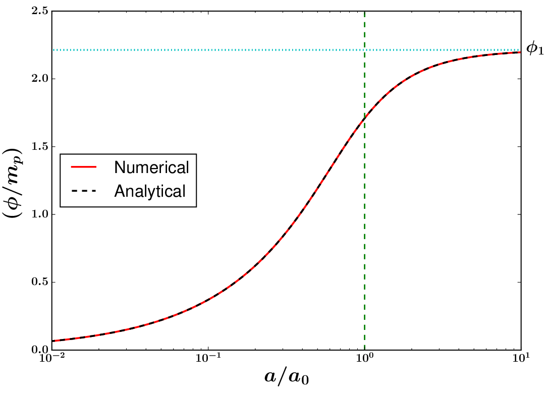
Integrating (21), one obtains the following exact solution22 2 The exact solution for can also be written as follows where is the Gauss hypergeometric function and is given in (31). for
| (28) |
where is a constant (having dimensions of mass) given by
| (29) |
and is an elliptic integral of the first kind, defined as
| (30) |
In obtaining (28) we have chosen the constant of integration such that . It is worth noting that starting from initially (when ), the scalar field rolls up to the following asymptotic value in the infinite future ()
| (31) |
where . The complete elliptic integral of the first kind is defined as .


Inverting equation (28) one can express the expansion rate in terms of as follows
| (32) |
where is one of the Jacobi elliptic functions 33 3 If , then the inverse is a Jacobi elliptic function.. Next, by inserting the expression for from (32) into (22), one easily gets the exact form for the reconstructed potential as
| (33) |
Using the properties of the concerned special functions, one can show that both (28) and (33) possess the correct limiting values given by (24) and (26) respectively.

The reconstructed potential in (33) is periodic in and its relevant part is plotted in figure 4 (red curve) for . The early and late time asymptotes, given by (24) and (26), are shown by the blue and green dashed curves respectively. Starting from its initial value (set at ) the scalar field rolls up to , given in (31), in the infinite future (). This is illustrated in figure 4 for . The potential has a minimum at , as shown in figure 4 by the vertical dotted cyan line. The scalar field rolls to that minimum very slowly in the infinite future ().
Figures 4 and 5 show that numerical simulations carried out using the potential (33) lead to precisely CDM-like expansion. Figure 5 demonstrates that the potential (33) possesses the same tracking feature as the inverse power law potential with alike large basin of attraction at early times, even within the braneworld framework. Therefore, the scalar field can mimick the expansion of a CDM universe while rolling on the potential (33), without requiring fine-tuned initial conditions.
It is interesting that although the braneworld and CDM have exactly the same expansion history, the two models can be easily distinguished on the basis of structure formation, since linearized density perturbations grow at different rates in the two models 44 4 Since the quintessence dark energy does not cluster on the brane in usual setup, the perturbation of the quintessential field can be ignored. Therefore, one can assume the quasi-static approximation [19] for calculating the growth of matter perturbation in late times on the phantom brane.. This has been illustrated in figure 6; also see figure 2 of [1].
IV Discussion
In this paper we have derived an expression for the dark energy density which, when residing on the phantom brane, causes the brane to expand like a CDM universe. We have also shown how DE can be related to a scalar field and derived a precise form for the scalar field potential . Interestingly, the potential possesses the same early time tracking feature as that of an inverse power law potential and the former can be well approximated by a -attractor potential. We have thus demonstrated that a scalar field propagating on the phantom-brane can make the latter mimic the expansion of CDM model.
It may be appropriate to note in this connection that braneworld expansion can mimic CDM even in the complete absence of dynamical dark energy on the brane. As shown in [20, 21] such a scenario of ‘cosmic mimicry’ [20] can arise in either of the following cases:
- •
The brane tension is large and there is a large cosmological constant associated with the bulk fifth dimension [20]. (The present treatment assumed that there was no -term associated with the bulk.)
- •
The brane violates symmetry with respect to the bulk [21]. In this case a small -term on the brane is induced by a slight asymmetry in values of the fundamental constants in the bulk.
Our present paper extends this previous work by constructing an entirely different scenario for cosmic mimicry.
Acknowledgments
The authors acknowledge useful discussions with Yu. Shtanov and A. Viznyuk. S.B. and S.S.M. thank the Council of Scientific and Industrial Research (CSIR), India, for financial support as senior research fellows.
References
- [1] F. Schmidt, Phys. Rev. D 80 123003 (2009) [arXiv:0910.0235].
- [2] V. Sahni and A.A. Starobinsky, Int. J. Mod. Phys. D9 373 (2000); P. J. E. Peebles and B. Ratra, Rev. Mod. Phys. 75 559 (2003); T. Padmanabhan, Phys. Rep. 380 235 (2003); V. Sahni, [astro-ph/0202076], [astro-ph/0502032]; V. Sahni, Dark matter and dark energy, Lect. Notes Phys. 653, 141-180 (2004) [astro-ph/0403324]; V. Sahni and A.A. Starobinsky, Int. J. Mod. Phys. D15 2105 (2006); E. J. Copeland, M. Sami and S. Tsujikawa, Int. J. Mod. Phys. D15 1753 (2006); R. Bousso, Gen. Relativ. Gravit. 40, 607 (2008); L. Amendola and S. Tsujikawa, Dark Energy, Cambridge University Press, 2010.
- [3] Ya.B. Zeldovich, Ya.B. Sov. Phys. – Uspekhi 11, 381 (1968).
- [4] S. Weinberg, Rev. Mod. Phys. 61, 1 (1989).
- [5] Planck 2015 results. XIV. Dark energy and modified gravity, P. Ade et al., arXiv:1502.01590.
- [6] T. Delubac et al. [BOSS Collaboration], Astron. Astrophys. 574 (2015) A59 doi:10.1051/0004-6361/201423969 [arXiv:1404.1801 [astro-ph.CO]]. A. Font-Ribera et al. [BOSS Collaboration], JCAP 1405 (2014) 027 doi:10.1088/1475-7516/2014/05/027 [arXiv:1311.1767 [astro-ph.CO]].
- [7] V. Sahni, A. Shafieloo and A.A. Starobinsky, Astrophys.J. 793 L40 (2014).
- [8] R.R. Caldwell, Phys. Lett. B 545, 23 (2002) [astro-ph/9908168]
- [9] J.M. Cline, S. Jeon and G.D. Moore, Phys.Rev. D70, 043543 (2004) [hep-ph/0311312].
- [10] V. Sahni and Yu.V. Shtanov JCAP 0311,014, (2003) astro-ph/0202346.
- [11] G. R. Dvali, G. Gabadadze and M. Porrati, Phys. Lett. B 485 (2000) 208 doi:10.1016/S0370-2693(00)00669-9 [hep-th/0005016].
- [12] U. Alam and V. Sahni, Phys. Rev. D73 084024 (2006) [astro-ph/0511473]; R. Lazkoz, R. Maartens and E. Majerotto, Phys. Rev. D 74 (2006) 083510 doi:10.1103/PhysRevD.74.083510 [astro-ph/0605701]. U. Alam, S. Bag and V. Sahni, Phys. Rev. D 95 023524 (2017) [arXiv:1605.04707].
- [13] V. Sahni, A. Shafieloo and A. A. Starobinsky, Phys. Rev. D 78 (2008) 103502 [arXiv:0807.3548 [astro-ph]].
- [14] A. Barreira, A. G. Sánchez and F. Schmidt, Phys. Rev. D 94 (2016) no.8, 084022 doi:10.1103/PhysRevD.94.084022 [arXiv:1605.03965 [astro-ph.CO]].
- [15] R. Kallosh and A. Linde, JCAP 1307 (2013) 002 doi:10.1088/1475-7516/2013/07/002 [arXiv:1306.5220 [hep-th]]. R. Kallosh, A. Linde and D. Roest, JHEP 1311 (2013) 198 doi:10.1007/JHEP11(2013)198 [arXiv:1311.0472 [hep-th]].
- [16] B. Ratra and P. J. E. Peebles, Phys. Rev. D 37 (1988) 3406. doi:10.1103/PhysRevD.37.3406
- [17] I. Zlatev, L. M. Wang and P. J. Steinhardt, Phys. Rev. Lett. 82 (1999) 896 doi:10.1103/PhysRevLett.82.896 [astro-ph/9807002].
- [18] S. Bag, S. S. Mishra and V. Sahni, arXiv:1709.09193 [gr-qc].
- [19] K. Koyama and R. Maartens, “Structure formation in the dgp cosmological model,” JCAP 0601, 016 (2006) [astro-ph/0511634]; S. Bag, A. Viznyuk, Y. Shtanov and V. Sahni, “Cosmological perturbations on the Phantom brane”, JCAP 1607 (2016) no.07, 038, doi:10.1088/1475-7516/2016/07/038 [arXiv:1603.01277 [gr-qc]].
- [20] V. Sahni, Yu. Shtanov and A. Viznyuk, JCAP 0512 (2005) 005 [astro-ph/0505004].
- [21] Yu. Shtanov, V. Sahni, A. Shafieloo, A. Toporensky, JCAP 0904 (2009) 023 [arXiv:0901.3074].