Power law observed in the motion of an asymmetric camphor boat under viscous conditions
Abstract
We investigated the velocity of an asymmetric camphor boat moving on aqueous solutions with glycerol. The viscosity was controlled by using several concentrations of glycerol into the solution. The velocity decreased with an increase in the glycerol concentration. We proposed a phenomenological model, and showed that the velocity decreased with an increase in the viscosity according to power law. Our experimental result agreed with the one obtained from our model. The results provided an approximation that the characteristic decay length of the camphor concentration profile at the front of the boat was sufficiently shorter than that at the rear of the boat, which was difficult to measure directly.
I Introduction
We can observe a wide variety of patterns, such as in a traffic jam [1, 2, 3], a large-scale ordering of swimming bacteria [4, 5], a swarm of mosquitoes, a parliament of birds and a school of fish [6, 7, 8], formed by living things as self-propelled objects. It is one of the challenging studies to understand pattern formations induced by these collective motions.
Similar behaviors also emerge in chemical systems, such as microtubes [9], droplets [10, 11, 12], Janus particles [13, 14] and camphor systems [15, 29, 16, 25, 26, 30, 15, 17, 18, 20, 21, 22, 31, 27, 18, 19, 28, 24, 23]. Self-propelled objects transform chemical energy into kinetic energy in non-equilibrium systems, and move spontaneously as if these were living. Recently, a lot of studies have reported on camphor boats as self-propelled particles in the chemical system [15, 16, 17, 18, 20, 19]. A camphor boat is made of a plastic sheet attached to a camphor disk. When the camphor boat is put on an aqueous surface, the camphor molecules dissolve from the disk under the boat and expand on the surface. As the camphor molecules decrease the surface tension of the aqueous phase, the camphor boat moves on the aqueous phase spontaneously due to a difference in surface tension around the boat. There have been many experimental studies, as well as numerical ones, on the camphor boat. Some of the numerical models are based on reaction-diffusion dynamics on the camphor concentration [20, 21, 22, 24, 23], and the others are based on fluid dynamics [25, 26, 27]. These models could explain the experimental behaviors in a qualitative manner. Basic physical quantities were necessary in order to realize the quantitative correspondence. However, it had been difficult to measure the driving force on the motion of the camphor boat, the surface tension difference between the front and the back of the boat, the diffusion coefficient, the supply rate of camphor molecules from the camphor disk to the water surface, and a relaxation rate before Suematsu et al. measured these quantitative properties in experiments [18]. The results have allowed us to compare the experimental results with theoretical ones quantitatively, and have provided a deep understanding of the interesting phenomena of the camphor boat. However, they investigated only the situation for pure water as an aqueous phase. Thus, we focused on viscosity dependence of the motion with regard to a camphor boat.
As methods to change the viscosities of the aqueous solution under the camphor boat, the temperature control of the solution or the use of the solution with different physical concentration is considered. We adopted the latter; we used aqueous solutions of glycerol with several glycerol concentration [21, 28], and changed the viscosity of the base solution.
In this paper, we investigated the velocity of the camphor boat for several glycerol concentrations , and found that decreased with an increase in . In order to understand the dependence of , we proposed the mathematical model. The model showed a power law , where is the viscosity of the base solution. Our experimental results satisfied the scaling relation obtained from the numerical model. The agreement between the experimental result and the theoretical result for the viscosity dependence of provides an estimation of the concentration field around the camphor boat, which is difficult to measure directly in experiments.
II Experimental procedure
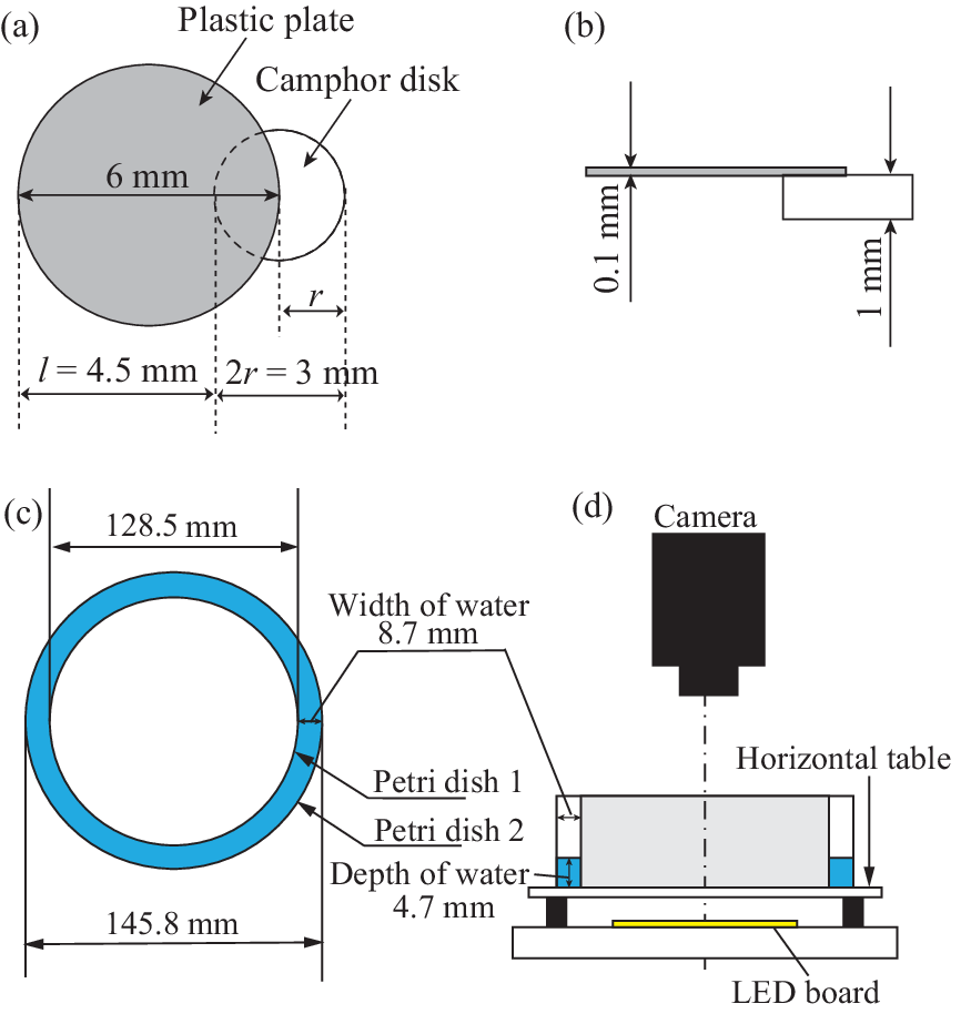
A round-shape boat as shown in Figs. 1(a) and (b) was used to measure the velocity of the camphor boat. The boat was composed of a plastic plate (thickness: 0.1 mm) and a camphor disk, which was prepared by pressing camphor powder ((+)-Camphor, Wako, Japan) using a pellet die set for the preparation of samples on Fourier transform-infrared (FT-IR) spectroscopy analysis. The diameter and the thickness of the camphor disk were 3.0 mm and 1.0 mm, respectively. The plastic plate was cut in a circle with a diameter of 6.0 mm, and the camphor disk was attached to the edge of the flat circular plastic plate using an adhesive (Bath bond Q, KONISHI, Japan), so that a half of the camphor disk was outside of the plastic sheet. This round-shape camphor boat moved toward the direction of the plastic sheet.
An annular glass chamber was used, which was composed of two petri dishes with different diameters as shown in Figs. 1(c) and (d). Inner and outer diameters were 128.5 mm and 145.8 mm, and the channel width of the chamber was thus 8.7 mm. As it is known that the velocity is sensitive to the depth of water [19], the chamber was put on the clear horizontal plate. The solution was poured into the chamber so that the depth of the solution was 4.7 mm, which was glycerol (Glycerol, Wako, Japan) and water mixed at several mass ratios , i.e. is a percentage of a glycerol mass in the mixed solution. We investigated physical properties of the solution, such as the viscosity, the surface tension, and the camphor solubility against glycerol concentration . The detailed results are shown in Appendix A. The camphor boat was put on the surface of the solution in the glass chamber, and then it started to move spontaneously. For a visualization of the motion, a LED board was placed under the horizontal plate. The motion of the boat was captured with a digital video camera (HDR-FX1, SONY, Japan) from the top of the chamber. Obtained movies were analyzed using an image-processing system (ImageJ, Nature Institutes of Health, USA).
III Experimental Results
We investigated the velocity of the camphor boat on the solutions of various glycerol concentration . The position of the camphor boat is described as a radial angle in the annular chamber, as shown in Fig. 2(a). Analyses of the videos captured by the digital video camera provide the position at time , where corresponds to the time when the boat finished three laps along the chamber after the boat had been put on the surface of the solution. In Fig. 2(b), had a constant gradient in time, that is to say, the camphor boat moved with a constant velocity. Figure 2(c) shows a time series of the angular velocity , where s for one frame of the video camera and is an angular difference between and . In Fig. 2(b), the expanded plot is shown for the time region corresponding to the gray region in Fig. 2(c). The angular velocity in the region fluctuated around the average value 1.08 rad/s. The similar tendency was observed at 50 s 200 s, i.e. increased with time and had noisy data before s, and began to decrease after s. Therefore, we investigated at 60 s 180 s, during which had almost a constant value for time. Next, we investigated the angular velocity for as shown in Fig. 2(d). The vertical and horizontal axes in Fig. 2(d) show the angular velocity and concentration . The was obtained from the linear fitting of time series as shown in Fig. 2(b). The values of the errors for each were lower than rad/s. As shown in Fig. 2(d), decreased with an increase in .

IV Mathematical Model
The glycerol concentration of the solution was controlled in our experiments, which led to a change in the viscosity shown in Appendix A. In this section, we consider a viscosity dependence of the camphor boat velocity. Now, the annular glass chamber used in our experiments is recognized as a one-dimensional channel with an infinite length.
The time evolution equation of the camphor boat in a one-dimensional system (The spatial coordinate is represented as ) is given as
| (1) |
where , , and are the mass, the center of mass, the friction coefficient of the camphor boat, and the driving force exerted on the moving camphor boat, respectively. We assume that is proportional to viscosity such as , where is a constant (). The assumption has been used in many previous papers [22, 28, 21, 20, 16, 15, 18, 17, 25, 23, 24], and it was also reported that the viscous drag on the mobility of thin film in Newtonian fluid obeyed a linear relationship with the fluid viscosity [32]. Therefore, we considered that the assumption is natural [33]. The driving force is described as
| (2) |
where is the width of the camphor disk. Here, we consider that the positions of the front and the back of the boat are shown as and , where and are the radius of the disk and the size of the boat as defined in Fig. 3. The surface tension depends on the concentration of the camphor molecules at the surface of the solution, and we assume the linear relation as
| (3) |
where is the surface tension of the base solution without camphor and is a positive constant.

The time evolution on the camphor concentration is shown as
| (4) |
where is the sum of sublimation rate and dissolution rate of the camphor molecules on solution surface, is the diffusion coefficient of the camphor molecule, and denotes the dissolution rate of the camphor molecules from the camphor disk to the aqueous solution surface. As for the term , we apply the following description,
| (5) |
That is to say, the dissolution of camphor molecules from the disk occurs at . The above equation does not include Marangoni effect directly, although the flow has an influence on the camphor concentration. The previous paper [31] showed that Eq. (4) was reasonable if was recognized as the spatially uniform effective diffusion coefficient of the camphor to include the transportation by the flow. In addition, this spatially-uniform effective diffusion coefficient is supported by the experimental results that the diffusion length is proportional to the square root of elapsed time [15].
V Theoretical analysis
Our experimental results showed that the camphor boat moved with a constant velocity in time as shown in Fig. 2. Thus, we should consider solutions for the motion of the camphor boat with a constant velocity in -direction, i.e. . From this condition, Eq. (1) leads to
| (6) |
By setting and , Eq. (4) provides
| (7) |
Equation (7) leads to the following solutions
| (8) |
where
| (9) |
| (10) |
| (11) |
| (12) |
| (13) |
VI Numerical results
In the theoretical analysis, we have assumed the solution depending on . However, the supposed mathematical model has other symmetries and whether the considered solution depending on is an attractor or not should be checked. Therefore, we performed numerical calculations based on equations in Sec. IV. For numerical calculation, we considered a one-dimensional array with a spatial step of . The spatial size of the considered system was 1000 with periodic boundary condition, and we adopted Euler method with time step As for the spatial derivative, we used explicit method. The parameters are set to be , , , , , , , and . In the discretization process, the first-order interpolation was adopted for Eqs. (2) and (5). The parameter corresponding to the viscosity was changed, and we investigated the time development of the camphor boat position and camphor concentration profile.

In Fig. 4, the numerical results are shown. In Fig. 4(a), the time development of camphor boat velocity is shown. The camphor boat velocity is saturated to a constant value. The camphor concentration profile after the velocity became constant () is shown in Fig. 4(b). The camphor concentration profile was asymmetric with regard to the camphor boat position . After reaching a constant velocity, the concentration profile did not change the shape but shifted in a positive -direction. Thus, we can guess that the solution with regards to is an attractor of this system. We have also confirmed that the solution converged to this attractor from other initial conditions (data not shown). The mathematical analysis on this convergence to the solution depending on remains and it may be possible to approach such mathematical problem by considering Lie group symmetry [35].
The final velocity against is shown in Fig. 4(c). For the regime of smaller than 0.1, the power law held, where is proportional to the viscosity in the present framework. In the theoretical analysis, we assumed and , which is equivalent to , as will be discussed in detail in the following section. Since the final velocity is nearly equal to 5 for , and , the divergence from the power law originates from the breakdown of the assumption in the analysis.
VII Discussion
Our model showed a power law under the assumptions that and . In this section, we compare experimental results with the numerical results in Eq. (17) in order to check whether our model is reasonable. Equation (17) has several parameters such as , , , , , and . Since similar camphor boats were used, , , and were constant values in our experiments. We investigated the dependence of the other parameters, i.e., , , and , on the glycerol concentration in Appendix A. Equation (3) showed . As was independent of in our measurements, we considered that was constant. The supply rate corresponds to , which is a loss of a camphor disk per unit time in our experiments, and we found that decreased with an increase in . The viscosity of the base solution increased with . Thus, and in Eq. (17) are functions of . In addition, the angular velocity is proportional to the camphor boat velocity in our experiments.
From the above discussion, Eq. (17) leads to
| (18) |
Figure 5 shows a relationship between and obtained from our experiments. The result almost agrees with the solid line in Eq. (18) [36].

The power law was obtained under the assumptions that and , which is equivalent to . Since corresponds to a characteristic decay length of the camphor concentration profile, and is a distance of the camphor boat motion during the characteristic time during which the concentration field keeps the memory, the assumption means that the characteristic length for the camphor concentration profile is sufficiently smaller than the characteristic length for the camphor boat motion. In such a case, the camphor concentration profile should be asymmetric with respect to the camphor particle position.
Here, we confirm the acceptability of the assumptions for our experiments. We needed values of parameters such as , , and included in the assumption. We used a rectangular camphor boat and chalk powders in measurements of . The boat was put on the solution surface covered by the chalk powders, and the camphor diffused into the solution. The diffusion was visualized by the chalk powders. We analyzed the videos of powders’ motion and estimated . A method of the measurement is similar to that in a previous study [18]. The effective diffusion coefficient against is shown in Appendix B, which shows that decreases with an increase in . For , s-1 was used, which was based on the experimental observation reported in the previous work [18]. Using these data, the relationship between and was obtained as shown in Fig. 6. The result shows that the values of were sufficiently smaller than 1 for all , which suggests that our assumption is reasonable. The result provides the following consideration: the camphor concentration around the boat is quite asymmetric, and the decay length of the concentration field at the back of the boat is sufficiently greater than that at the front.

There have been many analytical studies on collective motion of symmetric camphor disks in both experiments and theoretical analyses [16, 22, 30, 23]. There have also been some studies on asymmetric camphor boats, in which numerical calculation for both concentration field and camphor boat positions was performed, and analytical approach under the assumption of slow velocity was performed [15, 24]. In contrast to these studies, we discussed under the assumption of fast velocity, and this assumption was justified by the experimental observation. It would enable analytical approach on the collective motions of the camphor boats with fast velocity. Therefore, our model would provide a deep understanding of the collective motions on not only camphor boats but also living things.
VIII Conclusion
We investigated the velocity of the asymmetric camphor boat against several glycerol concentration of the glycerol aqueous solution. In order to know the dependence of the camphor boat velocity on the glycerol concentration , we discussed a numerical model based on a diffusion-reaction equation. When it is assumed that the characteristic length of the camphor concentration at the front of the boat is shorter than that at the rear, should obey a power law , where is the viscosity of the base solution. The power law agreed with experimental results, and it was also confirmed that our assumption in the model was reasonable through a comparison with our experimental results. Using our proposed model, we can discuss the profile of camphor concentration, which is difficult to be directly measured in experiments. Thus, our experiment has profound significance in the estimation of the concentration through the measurements of the velocity.
As a future topic, it would be worth investigating whether the similar power law persists with smaller levels of in experiments with such variables as increased the boat size. In addition, we considered that the hydrodynamic effect was included in the effective diffusion coefficient in this paper. It, however, would be also important to consider the fluid flow around the boat when we study the behavior of two or more camphor boats as the collective motion. As future work, it would be also interesting to consider the hydrodynamic interaction in multi camphor particle system.
Acknowledgements.
This work was supported by Y. Koyano. MS would like to thank Samantha Hawkins of Fukuoka Institute of Technology for proofreading this manuscript. This work was supported by JSPS KAKENHI Grant Numbers JP18K11338, JP18K03572, JP25103008 and JP15K05199.Appendix A Physical properties of a glycerol-water solution as a base solution
Figure 7(a) shows a viscosity dependence for various glycerol concentrations of the aqueous solution; i.e. means a percentage of a glycerol mass in the aqueous solution. The viscosity was measured using a viscometer (SV-10A, AD, Japan). As shown in Fig. 7 (a), the viscosity increased with .
Figure 7(b) shows surface tension difference of the solution for , where and correspond to the surface tension for glycerol-water solution without camphor and that for the solution with g camphor dissolved per 1500 ml, respectively. The camphor concentration was set to become close to that in measurements of angular velocity . The surface tension was measured using a surface tensiometer (DMs-401, Kyowa Interface Science Co., Ltd., Japan). The surface tension with camphor was lower than that of without the camphor, and and decreased with an increase in glycerol concentration . The difference of , however, almost kept constant for different values of as shown in Fig. 7 (b). The average value of was 0.29 mN/m.
Next, we investigated the dependence of camphor solubility on the glycerol concentration of the base solution. We measured the mass of the camphor disk before and after the camphor disk moved for min, and the mass change was set to be . From , we obtained the weight loss rate . As shown in Fig. 7 (c), decreased with an increase in .

Appendix B Effective diffusion coefficient of camphor on solution with several glycerol concentrations
The effective diffusion coefficient of camphor is included in our assumption, and the value of was necessary for checking whether the assumption was reasonable. Thus, we measured for various glycerol concentrations .
The rectangular boat in Figs. 8(a)-(d) was used for the measurements of the effective diffusion coefficient of the camphor molecules on the solution, and its shape was different from the round-shaped boat in the measurements of the velocity. The rectangular boat was made by bending both sides of a rectangular plastic plate that was 8.0 mm in width and 10.0 mm in height at 2.0 mm from the edge. The camphor disk was attached at the center of the plastic plate, where the shortest distance from the edge was 3.5 mm. The shape was similar to the one reported in the previous study [18].

Figures 9(a)-(f) are snapshots captured from the top at time , where (a) s, (b) 0.03 s, (c) 0.07 s, (d) 0.13 s, (e) 0.20 s and (f) 0.30 s, respectively. In Fig. 9, corresponds to the time at which the chalk powders started moving on the water. The diffusion of camphor molecules under the rectangular boat leads to the motion of chalk powders on the water surface. As shown in Fig. 9(a), all regions of the surface were covered by chalk powders with a gray color at . The chalk powders started moving at s, and the water surface without powders was observed as a white region around the boat in Fig. 9(b). The area of the white region grew with time (Figs. 9(b)-(d)). The boat stayed at the same position before s (Figs. 9 (a)-(e)), although the powders moved. The camphor boat, then, started to move after s (Fig. 9(f)). In this process, the chalk powders were carried by not only the camphor diffusion but also fluid flow induced by the motion of the boat.


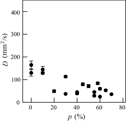
Next, we investigated at time , where was the longest distance between the edge and the center of the region with the camphor layer, shown as the white region in Fig. 9. The closed circles, open squares and closed triangles in Fig. 10(a) show the data for ( 0.92 mPas) for water, and ( mPas) and ( mPas) for the glycerol-water solution, respectively. Let us focus on the data for . The trend of the data changed around at s, which almost corresponded to the time when the camphor boat began to move as shown in Fig. 9. As we needed the effective diffusion coefficient of the camphor, we measured in the time range in which the camphor boat did not move. Figure 10(b) is an expanded figure for small , i.e. time without the boat motion. When the camphor boat stayed at a certain position, increased linearly with time. Linear fittings are shown as solid lines, where fitting was executed for the region 0 s 0.13 s for closed circles. The gradients of these solid lines provide the effective diffusion coefficients of the camphor molecules on the glycerol-water solution. The effective diffusion coefficient on the water was obtained at mm2/s. A previous paper [31] reported that the effective diffusion coefficient in a numerical study almost agreed with the value for measured with this method. Thus, we consider that this method is reasonable for the measurement of . The gradient of the solid line decreases with an increase in the glycerol concentration. Figure 11 shows the relationship between and , and the tendency that decreases with an increase in was confirmed.
References
- [1] A. Nakayama, et al., New J. Phys. 11, 083025 (2009).
- [2] M. Bando, et al., Phys. Rev. E 58, 5429 (1998).
- [3] Y. Sugiyama, et al., New J. Phys. 10, 033001 (2008).
- [4] C. Peng, et al., Science 354, 882 (2016).
- [5] D. Nishiguchi, et al., Phys. Rev. E 95, 020601(R) (2017).
- [6] T. Vicsek, et al., Phys. Rev. Lett. 75, 1226 (1995).
- [7] T. Vicsek and A. Zafeiris, Phys. Rep. 517, 71 (2012).
- [8] J. Toner and Y. Tu, Phys. Rev. Lett. 75, 4326 (1995).
- [9] Y. Sumino, et al., Nature 483, 448 (2012).
- [10] S. Thutupalli, R. Seemann, and S. Herminghaus, New J. Phys. 13, 073021 (2011).
- [11] T. Ohmura, et al., Appl. Phys. Lett. 107, 074102 (2015).
- [12] S. Tanaka, S. Nakata, and T. Kano, J. Phys. Soc. Jpn. 86, 101004 (2017).
- [13] D. Nishiguchi, et al. New J. Phys. 20, 015002 (2018).
- [14] J. Hu, et al. Chem. Soc. Rev. 41, 4356 (2012).
- [15] N. J. Suematsu, et al., Phys. Rev. E 81, 056210 (2010).
- [16] H. Nishimori, N. J. Suematsu, and S. Nakata, J. Phys. Soc. Jpn. 86, 101012 (2017).
- [17] M. I. Kohira, et al., Langmuir 17, 7124 (2001).
- [18] N. J. Suematsu, et al., Langmuir 30, 8101 (2014).
- [19] Y. Matsuda, et al., Chem. Phys. Lett. 654, 92 (2016).
- [20] S. Nakata, et al., Phys. Chem. Chem. Phys. 17, 10326 (2015).
- [21] M. Nagayama, et al., Physica D 194, 151 (2004).
- [22] E. Heisler, et al., J. Phys. Soc. Jpn. 81, 074605 (2012).
- [23] K. Nishi et al., Phys. Rev. E 92, 022910 (2015).
- [24] E. Heisler, et al., Phys. Rev. E 85, 055201 (2012).
- [25] S. Soh, K. J. M. Bishop, and B. A. Grzybowski, J. Phys. Chem. B 112, 10848 (2008).
- [26] S. Soh, M. Branicki, and B. A. Grzybowski, J. Phys. Chem. Lett. 2, 770 (2011).
- [27] E. Lauga and A. M. J. Davis, J. Fluid Mech. 705, 120 (2011).
- [28] Y. Koyano, H. Kitahata, and T. Sakurai, Phys. Rev. E 94, 042215 (2016).
- [29] N. J. Suematsu, et al., J. Phys. Soc. Jpn. 84, 034802 (2015).
- [30] Y. S. Ikura, et al., Phys. Rev. E 88, 012911 (2013).
- [31] H. Kitahata and N. Yoshinaga, J. Chem. Phys. 148, 134906 (2018).
- [32] H. A. Stone and H. Masoud, J. Fluid Mech. 781, 494 (2015).
- [33] It would be interesting to investigate the viscous dependence for a viscous drag directly in a similar experiment to Ref. [18].
- [34] J. Happel and H. Brenner, Low Reynolds number hydrodynamics: with special applications to particulate media (Springer, 1983).
- [35] P. J. Olver, Applications of Lie groups to differential equations (Springer, 1993).
- [36] The experimental data are distributed since the values of are noisy as shown in Fig. 7(c) of Appendix A. The values of , investigated in the motion of the camphor disk, are sufficiently small to be susceptible to external factors.