Rigorous Asymptotic Models of Water Waves
Abstract. We develop a rigorous asymptotic derivation of two mathematical models of water waves that capture the full nonlinearity of the Euler equations up to quadratic and cubic interactions, respectively. Specifically, letting denote an asymptotic parameter denoting the steepness of the water wave, we use a Stokes expansion in to derive a set of linear recursion relations for the tangential component of velocity, the stream function, and the water wave parameterization. The solution of the water waves system is obtained as an infinite sum of solutions to linear problems at each level, and truncation of this series leads to our two asymptotic models, which we call the quadratic and cubic -models.
Using the growth rate of the Catalan numbers (from number theory), we prove well-posedness of the -models in spaces of analytic functions, and prove error bounds for solutions of the -models compared against solutions of the water waves system. We also show that the Craig-Sulem models of water waves can be obtained from our asymptotic procedure and that their WW2 model is well-posed in our functional framework.
We then develop a novel numerical algorithm to solve the quadratic and cubic -models as well as the full water waves system. For three very different examples, we show that the agreement between the model equations and the water waves solution is excellent, even when the wave steepness is quite large. We also present a numerical example of corner formation for water waves.
1 Introduction
Both gravity and capillary water waves are modeled by the free-surface incompressible Euler equations of fluid dynamics, and for many applications, the fluid is additionally assumed to be irrotational. Well-posedness, stability, and singularity formation have been well studied with many results; see, for example, [52, 71, 26, 13, 11, 68, 69, 70, 8, 46, 47, 22, 61, 21, 19, 6, 40, 33, 42, 41, 7, 17, 23, 31, 24, 28]. However, the Euler equations are sufficiently complicated that for many physical scenarios, a precise understanding of the dynamics of the solutions to the full water waves problem is not (at this time) known. Consequently, since the pioneering works of Airy, Boussinesq and Stokes [1, 14, 15, 64], there has been a sustained effort to find suitable approximations of the Euler equations, specific to certain asymptotic regimes. Such approximate asymptotic models have closely related dynamics and can be significantly easier to analyze. Herein, we develop an asymptotic procedure that yields approximate model equations for the water waves problem to various orders of approximation of the nonlinearity. In particular, we present two models that respectively capture the nonlinearity up to quadratic and cubic interactions.
We derive two asymptotic models for the evolution of both gravity and gravity-capillary waves in deep water, using an asymptotic expansion in the steepness of the wave , which we view as a small parameter, equivalent to the ratio of the amplitude to the wavelength. Such an expansion has been used extensively since it was introduced by Stokes [64]; see, for example, [3, 53, 54, 4, 5]). Starting with the case of gravity water waves, we employ such a Stokes expansion and obtain linear recursion relations for the stream function, the tangential component of velocity, and the free-surface parameterization. Truncating this expansion to yields a quadratic model equation for gravity water waves. We refer to this PDE as the quadratic -model
| (1) |
Keeping all terms in the recursion relation to yields the cubic -model, a new model of water wave dynamics that accurately captures the cubic interactions of the Euler equations and is given by
| (2) |
where the cubic nonlinearity is defined in (63). Asymptotic models for gravity-capillary waves are derived in the same fashion (in section 5.3) when gravity and surface tension forces are of the same order.
The same expansion procedure that we used for the one-fluid problem can be used to derive models for two-fluid internal waves and the Rayleigh-Taylor instability (as noted in Remark 2). Furthermore, out approach can be applied to the case of finite depth fluids as well.
We note that the quadratic -model was first derived by Akers & Milewski [2] using a formal asymptotic procedure in which they assumed that due to very small amplitudes of the water wave, it could be assumed that all elliptic problems are set on the time-independent half-space. A Stokes expansion procedure was then used by Akers & Nicholls [3] with a time-dependent fluid domain, but for the case of the traveling wave ansatz.
We prove that both the quadratic and cubic -models are well-posed in spaces of analytic functions that are similar to the Wiener algebra but with a (growing) exponential weight (used to guarantee analyticity). As we noted above, our methodology relies upon a sequence of linear recursion relations obtained via the Stokes expansion, and thus it is possible (in principle) to solve a nonlinear PDE by a summation of an infinite series, each term in the series coming from a solution to a linear problem. The objective, then, is to prove summability of the infinite series; however, classical contraction mapping techniques fail due to the growth of the norm of the th linear solution. Remarkably, the growth of these norms can be quantified and estimated in terms of the Catalan numbers [63] from number theory (which are often used in combinatorics), and the well-known bounds on the Catalan numbers then permit the convergence of the infinite series to the solution of the nonlinear problem.11 1 It may be possible to establish existence of solutions to the -models using some type of Cauchy-Kovalevsky theorem, but we are not aware of a particular form of the theorem that would be directly applicable. We also establish rigorous error bounds for the difference between solutions of the -models and the full water waves system. We thus conclude that both the quadratic and cubic -models are accurate asymptotic models of water waves in the small -regime.
The asymptotic procedure that we shall describe below allows us to derive a large class of asymptotic models of water waves, including the well-known hierarchy of models obtained by Craig & Sulem [27]; in particular, we show that their most studied model, WW2 (or water waves 2), is obtained from our approach, and we prove that it too is well-posed in spaces of analytic functions. Moreover, we write the WW2 model as a second-order wave equation and explain its connection with the quadratic -model.
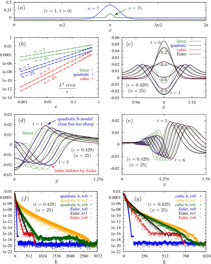
Finally, we present an arbitrary-order exponential time differencing scheme [25, 44, 18] for solving the quadratic and cubic -models accurately and efficiently and compare those solutions against numerical solutions of the Euler equations. We show that the -models converge as expected: with denoting the maximum slope of the initial condition, the quadratic and cubic -models converge in to solutions of the full water waves problem with rates and , respectively, where the error is scaled by to account for the decreasing (as a function of ) norm of the exact solution. We give three examples of initial data that show excellent agreement between the -models and the full water waves solution all the way up to . The first example is a multi-hump initial condition in which a jet forms in each trough as the solution drops from rest; the second example is a localized disturbance over a flat surface that propagates outward as time evolves; and the third example is a family of standing water waves. In all three cases, the quadratic and cubic models are much better than linear theory at capturing features of the dynamics. For large , the quadratic model has a tendency to form a corner singularity while the cubic model tracks the Euler solution quite well. We also present a continuation of the first example for the Euler equations to show that the wave eventually overturns and appears to form a corner singularity before self-intersecting, with at the tip of one of the overturning waves.
Paper Outline. In Section 2, we introduce the notation and some important definitions used throughout the paper. In Section 3, we introduce the water waves equations, and the three fundamental variables that shall be evolved: the tangential component of velocity, the stream function, and the free-surface parameterization. Section 4 is devoted the Stokes expansion of the water waves system and the derivation of the linear recursion relations. In Section 5, we derive the quadratic and cubic -models, and in Section 6, we prove that these models are well-posed. In Section 7, we derive the Craig-Sulem WW2 model, and prove that it too is well-posed. Section 8 establishes the error estimates for solutions of the -models compared to the full water waves system. Then, in Section 9, we perform a number of numerical experiments that compare the quadratic and cubic -models with a highly accurate numerical solution of the full water waves system.
2 Some notation and definitions
2.1 Matrix indexing
Let be a matrix, and be a column vector. Then, we write for the component of , located on row and column ; consequently, using the Einstein summation convention, we write
2.2 Power series summation
We adopt the convention that independent of the summand ,
| (3) |
2.3 The water wave parameterization
We identify with the interval . We shall denote a general parameterization of the free-surface of the fluid by the diffeomorphism . This free-surface of the fluid is the water wave, which we denote by . Hence, the water wave is given by
For the majority of our analysis, we shall assume that the water wave evolves as a graph over the horizontal -axis. in particular, and
| (4) |
The one-to-one function is often called the signed height function.
2.4 The fluid domain and some geometric quantities
The time-dependent fluid domain is defined as
| (5) |
i.e. for the sake of simplicity, we assume that the depth of the fluid is much larger than the amplitude of the wave.
We define the reference domain as
| (6) |
We let denote the outward unit normal to , and we let and denote, respectively, the unit tangent and normal vectors to the water wave , where points outward to the set . We then set
When the water wave is defined by graph parameterization (4), the induced metric is given by
| (7) |
2.5 Derivatives
We write
and for a vector ,
The Laplace operator is defined as .
2.6 Fourier series
If is a square-integrable -periodic function, then it has the Fourier series representation for all , where the complex Fourier coefficients are defined by . We shall sometimes write for . Functions (which are square-integrable in can be expanded as for all , where .
2.7 Singular integral operators
Let denote a periodic function on . Using the Fourier representation, we define the Hilbert transform and the Dirichlet-to-Neumann operator as
| (8) |
In particular, we note that
Equivalently, suppose that is a periodic function and that is its harmonic extension to . Then,
| (9) |
Finally, we denote the commutator between and the Hilbert transform acting on as
Let us observe that
2.7.1 Function spaces
For , we denote by the set of Lebesgue measurable -periodic functions such that where if and . For integers , we let . For , we then define the space to be the -periodic distributions such that .
For a given , we define the following Banach scale of analytic functions as
| (10) |
3 Water waves equations
Water waves are modeled by the incompressible and irrotational free-surface Euler equations, written as
| (11a) | ||||||
| (11b) | ||||||
| (11c) | ||||||
| u | (11d) | |||||
| (11e) | ||||||
where , is defined in (5), is defined in (4), is the surface tension parameter and means that the free-surface moves with normal velocity . We shall assume that all functions are -periodic in .
3.1 The Bernoulli equation
Since in , for some scalar potential . Then, (11a) can be written as
| (12) |
where is a function independent of .
3.2 The evolution of the tangential velocity
On , we define the following quantities:
We shall make use of the tangential velocity
From (11e), so that
| (13) |
for an arbitrary scalar function . (Note that is a tangent vector and that the water waves problem has a tangential reparameterization symmetry.)
By the chain rule,
| (14) |
and
From (14), , and (13) shows that
Therefore, we find that satisfies
| (15) |
From (12),
so that
where we have used the boundary condition (11c) in the last equality. Using (15), we find that
| (16) |
We now suppose that the interface remains a graph and is given by (4). With the definition of the metric (7), we write the unit normal and tangent vectors, respectively, to as
Using (11e), we decompose v as follows:
| v | (17) |
and hence
| (18) |
Equations (13) and (17) then provide us with the identity
so that (16) can be written as
| (19) |
3.3 The equation for the stream function
Since is simply connected, by classical Hodge theory, we can uniquely determine the velocity vector u by solving the following elliptic system:
| (20) |
3.4 The evolution equation for the free-surface
4 Stokes expansion and linear recursion for the time-dependent water waves
4.1 Stokes expansion
Letting denote the steepness parameter (which can be viewed as the ratio of the amplitude to characteristic wavelength), we consider the following Stokes expansion ansatz:
| (25) |
where
| (26a) | ||||
| (26b) | ||||
| (26c) | ||||
In particular, at the initial time , we have
| (27) |
or, equivalently,
| (28) |
4.2 Linear recursion for the stream function
Using (23), the scalar Neumann problem (21) can be written as
| (29a) | ||||||
| (29b) | ||||||
and in expanded form,
| (30a) | ||||||
| (30b) | ||||||
Substitution of our Stokes expansion (25) shows that (30) is equivalent to the following linear recursion relation for :
| (31a) | ||||||
| (31b) | ||||||
4.3 Linear recursion for the height function
4.4 Linear recursion for the tangential velocity
In absence of surface tension effects (), we have that (19) is equivalent to
| (33) |
5 Derivation of the quadratic and cubic -models
5.1 Preliminary lemmas
The linear recursion for the stream function given in (31) can be decomposed into simpler elliptic equations. Thus, given certain forcing functions and , we shall focus on the following two elliptic equations
| (35) |
and
| (36) |
We shall make use of two lemmas that show that the restriction of the solutions of (35) and (35) to can be expressed in terms of the functions on : and .
Following our discussion in Section 2.6, a harmonic function in can be expanded as
for some complex coefficients that do not depend on . For example, the stream function , solving (31) with , is harmonic and hence . For , the right-hand side of (31a) is given by
and the right-hand side of (31b) is
It follows that the solution can be written via the expansion
where denotes the double sum and is a (double) sequence of complex numbers. Using the recursion formula (31), an induction argument then shows that for all , the stream function can be written as the expansion
where for each fixed , is a polynomial (of degree ) function of . This motivates the following two lemmas.
Lemma 1.
Let and denote -periodic functions of , such that
where is a polynomial function. If is the unique solution to (35), then
| (37) |
where denotes evaluated at . Moreover, if is harmonic in so that , then
| (38) |
where denotes the commutator.
Proof.
With , satisfies the differential equation
whose solution is given by the variation-of-parameters formula: for ,
Therefore,
| (39) |
and (37) follows from the Fourier inversion formula.
Lemma 2.
Proof.
Letting , we find that
The solution for the case is obtained via the variation-of-parameters formula as
Therefore,
which is (40).
5.2 The quadratic -model
From (31),
| (41) |
and
| (42) |
We decompose , where and satisfy
| (43a) | ||||||
| (43b) | ||||||
and
| (44a) | ||||||
| (44b) | ||||||
We note that the solvability condition for (43) is satisfied since integration-by-parts shows that
and similarly the solvability condition for (44) is also satisfied: . With the solvability conditions satisfied, the elliptic problems (43) and (44) have unique solutions in by the Lax-Milgram theorem. Using the Hilbert transform,
| (45) |
We can then apply Lemma 1 and conclude that
| (46) |
From the recursion for the tangential velocity and (32), we have that
| (47a) | ||||||
| (47b) | ||||||
| (47c) | ||||||
| (47d) | ||||||
We can write (47) as system of wave equations,
| (48a) | ||||
| (48b) | ||||
where, in the last equality, we have used the Tricomi identity
| (49) |
The quadratic -model follows from setting
| (50) |
so that
Neglecting terms of order , the quadratic model reads
| (51a) | ||||
| (51b) | ||||
The quadratic -model (51) modeling gravity water waves in deep water reduces to the “Model” equation obtained by Akers & Milewski [2], although in a very different way. They first simplify the water waves problem by making the assumption that the potential function at each recursion relation is set on the fixed domain with top boundary given by (rather than ). It is interesting to note that up to quadratic nonlinearity, this simplification produces the same -model as we have obtained by keeping the full water waves system in the asymptotics. We note that Akers & Nicholls [3] later used a diffeomorphism (similar to our ) to fix the domain, but only study the linear recursion for the traveling solitary wave ansatz.
Remark 1.
We observe that the quadratic -model (51) is kept invariant by the scaling
This is the same scale invariance as for the full gravity water wave problem.
Remark 2.
Following a similar approach, for the case of an internal wave separating two perfect fluids with densities and , we can derive the equation
| (52) |
where
is the Atwood number.
A similar asymptotic model was derived in Granero-Belinchón & Shkoller [35] to study the two-fluid problem.
5.3 The quadratic -model with surface tension
For surface waves in the regime where the effects of both gravity and surface tension are similar in magnitude (wavelengths of order or, equivalently, the Bond number ), the previous recursion for the tangential velocity has to be changed. This is somewhat challenging for general due to the denominator present in the expression for the mean curvature; however, for and this modification takes the following form:
| (53a) | ||||||
| (53b) | ||||||
| (53c) | ||||||
| (53d) | ||||||
Equivalently, taking a time derivative, we have that
Then, a similar argument as before shows that, up to , the quadratic model (51) with surface tension modeling gravity-capillary waves in deep water is written as
| (54) |
5.4 The cubic -model
In order to derive the cubic h-model, we shall also need the equation that satisfies; thus, in addition to (41) and (42), we use (31) to find that
| (55a) | ||||||
| (55b) | ||||||
We decompose as the sum , where , , and satisfy
Note that on .
Solving (41), , and by Lemma 1,
| (56) |
Next, we write the solution to (44) using the Fourier components , and using the variation-of-parameters solution to (43), we see that
thus,
It then follows from Lemma 1 with that
| (57) |
Using Lemma 2 with (or equivalently with ), we find that
| (58) |
Hence, combining (56), (57) and (58) and the fact that on ,
Noting that for each fixed ,
we have that
Therefore, we have that
| (59a) | ||||
| (59b) | ||||
We next time-differentiate (59a) and substitute (59b) to find that
Thanks to the identities in (47), we conclude that
Thus,
Using Tricomi’s identity (49), we can reduce the previous expression to
The cubic -model follows from setting
so that
Then, we find that
We observe that
thus, we can simplify the equation as follows:
We also compute that
so that
| (60) |
Using Tricomi’s identity for two functions, we find that
| (61) |
Grouping terms further using (60) and (61), together with
we obtain that
The cubic model is then given by
Therefore,
| (62) |
Making use of the commutator identities in Appendix A, the cubic nonlinearity can be written as
| (63) |
6 Well-posedness of the -models
In this section we develop a well-posedness theory for the quadratic and cubic models. In particular, we prove local well-posedness in the Wiener spaces (10) for the quadratic model (51) and the cubic model (62).
To prove these results, we use the linear recursion derived in (68) and (69). For the Navier-Stokes equation, the idea of using an asymptotic expansion together with the diffusive properties of the semigroup to prove well-posedness goes back to Oseen [55] and Knightly [45]. However, in our case, the model is hyperbolic and, consequently, there is no diffusive properties of the semigroup. Furthermore, as we consider the case of periodic waves, the semigroup does not have dispersive effects either. Instead of relying upon smoothing properties of the semigroup, we use the structure of the nonlinearity. This structure allow us to write an inequality for the -norms (10) that resembles the recursion for the Catalan numbers . These numbers can be defined recursively as
| (64) |
Then, we finalize the argument using well-known growth rates of the Catalan numbers. This idea of using the structure of the nonlinearity and the Catalan numbers is, to the best of our knowledge, new to the analysis of water waves models (an wave equations in general).
We remark that a closely related two-fluid asymptotic model derived in [35] has been shown to be well-posed in Sobolev spaces when the initial data satisfies a certain sign condition. In particular, in the case that for each point on the free-surface, that model is locally well-posed for arbitrary data and globally well-posed under certain size restrictions (see Theorems 7.1 and 7.6 in [35]).22 2 The condition can occur globally with certain in-flow boundary conditions. It is possible that the quadratic -model is also well-posed in Sobolev spaces when this sign condition holds for the initial data, and we plan to investigate this in future work.
6.1 Well-posedness theory for the quadratic -model
Using the ansatz (25), the quadratic model (51) can be written as
| (65) |
with initial conditions (28). We expand as in (26) for functions to be determined. Substituting into (65) we find that
| (66) |
with initial conditions
| (67) |
Using the Fourier series expansion, (66) shows that each Fourier component satisfies the differential equation
| (68) |
where is given by
| (69) |
We note that integration of (66) shows that
| (70) |
Solving the ODE (68) for , we find that
Similarly, the solution to (68) for is
and hence
| (71) |
Using the expression (69), we have that for , and verify the following recursion relations:
| (72) |
and
| (73) |
We now establish our existence theory for the quadratic h-model, and simultaneously prove that the Stokes expansion converges.
Theorem 3.
Proof.
Existence. We fix such that
Given , we seek solutions of (51) having the form
| (74) |
The series in (74) are respectively bounded by
| (75) |
Thus, by proving the boundedness of (75), we obtain the absolute convergence of (74) and, in particular, the existence of solutions to (51).
To obtain the required estimates, we first consider the truncated series (for )
Using (72), we have that
where we have used Tonelli’s theorem together with the fact that , which follows from (70), and the important inequality
| (76) |
Using (73), we can find a similar bound :
Since , it follows that
Similarly, if , then and
Then, we have that
| (77) |
We define
Next we show that for ,
| (78) |
Note that (78) clearly holds for . When ,
Similarly, when ,
Thus, (78) holds for , and this further implies that
We then obtain that the previous recursion for can equivalently be stated as
We observe that
| (79) |
Then, we want to prove by induction that
| (80) |
where are the Catalan numbers (64). Remarkably, the Catalan numbers as [63, page 136].
Having already established that (80) holds for , we proceed with the induction step. For we have that
Thus, using the asymptotic growth of the Catalan numbers, we have that
Analogously,
We define the series
Then
Similarly,
We conclude that if
then we can take the limit in and we compute that
Our estimates lead to
Moreover, using the Cauchy product of power series, we have that
where
Since and are analytic functions in space, using the previous expression, we obtain that and satisfy
In particular, they are continuous functions in time, .
Uniqueness. Let us assume that there exist two solutions emanating from the same initial data. Then, the difference
satisfies
with
Then, following the same argument as in the previous section, we expand , as in (71) and find that , satisfy the cascade of linear problems (68) and (69). Equivalently, we have that
satisfies
with
As before, we consider such that and define
Following the arguments in the previous section, we find that
Due to the previous inequalities, we prove that using induction and we conclude the uniqueness.
Remark 3.
Let us emphasize that the estimate is independent of . Thus, an appropriate passage to the limit allows for analytic initial data whose Fourier series has unbounded support. The argument to prove this generalization is straightforward and we leave it for the interested reader.
6.2 Well-posedness theory for the cubic -model
As we have seen, the cubic model can be written as the following nonlinear wave equation (62)
where is defined in (63). Using the ansatz (25), the cubic model (62) can be written as
| (81) |
with initial conditions (28). We again consider the expansion The quadratic nonlinearity follows as in (66). It thus suffices to expand the cubic nonlinearity. We define
| (82) |
Our starting point is the linear recursion (83) and (82). Similarly, the solution to (83) for verifies
| (84) |
and
| (85) |
where is the Fourier transform of the (linear) forcing
| (86) |
where is given by (82).
Theorem 4.
Proof.
The proof of this Theorem is similar to the proof of Theorem 3. As before, we fix such that
and consider . We need to estimate . Using the previous ideas in the proof of Theorem 3 together with (76) and the trivial identity
we have that
As before, we have that, for
Thus, we can estimate
Recalling (77), we find that
We define
Then, we can conclude that
We assume that . Recalling (79), and the fact that for the Catalan numbers (64) we have that
we can prove by induction that
Using this bound, we can conclude the existence and uniqueness as in Theorem 3.
7 The Craig-Sulem WW2 model
Zakharov [72] formulated the water waves problem as the following system of one-dimensional nonlinear and nonlocal equations:
| (87a) | ||||
| (87b) | ||||
where is the free surface, is the trace of the velocity potential on the free surface
and is the Dirichlet-Neumann operator
| (88) |
As a way to numerically simulate the evolution of water waves when surface tension is neglected, Craig and Sulem [27] gave a power series expansion for the Dirichlet-to-Neumann operator (88) as33 3 This type of expansion for the Dirichlet-to-Neumann operator was first used in electromagnetism by Milder [48] and Milder & Sharp [49].
| (89) |
with
By keeping terms up to certain order in the previous expansion (89) and starting from the Zakharov formulation (87), Craig and Sulem obtained a hierarchy of new truncated series models of the water waves problem. For instance, when we keep the terms up to second order, and , we obtain the WW2 (water waves 2) system
| (90a) | ||||
| (90b) | ||||
We define
| (91) |
Similarly, defining as in (50) and (91), respectively, and using (47) we have that
Then, neglecting terms of order and considering surface tension effects, from (47) we obtain the following coupled transport equations
| (92a) | ||||
| (92b) | ||||
These equations are the WW2 system obtained by Craig & Sulem writen in the variable Thus, our method is also able to recover the WW2 system. Similarly, following our previous ideas we can prove the following result for the WW2 Craig-Sulem system:
Theorem 5.
Let and the initial data be given. Assume that there exists such that
Then there exists a unique analytic solution to (92) for in the time interval with
In the following we are going to write the WW2 Craig-Sulem model as a wave equation. For an arbitrary function , we define the operator
The following inequalities hold
We define the following Neumann series
Then, if we have that
so, denoting by where the identity operator, we have that is invertible and
We observe that (92a) is equivalent to
Using the previous operators, we find the following equivalent formulation of the Craig-Sulem WW2 model as a nonlinear wave equation:
| (93) |
where the cubic and higher nonlinearities are contained in
| (94) |
and the operator is defined as
8 Estimating the difference between the models and the solution of the full water waves problem
In this section we estimate the error of solutions of the -models to solutions of the full water waves system.
Let be a initial data and consider its corresponding local solution to the full water waves problem in . As we described in the introduction, the well-posedness of the water waves problem is well-known (see the works by Ovsjannikov [56] and Shinbrot [62] for the case with analytic initial data), and that solutions exists for a lifespan . We have the following
Theorem 6.
Let , and the initial data be given. Assume that there exists such that
Denote by the local solution in of the full water waves problem starting from the initial data and let denote the solution to the quadratic model (51). Then, as long as both solutions exist,
Proof.
Analogously, we have that
Theorem 7.
Let , and the initial data be given. Assume that there exists such that
Denote by the local solution in of the full water waves problem starting from the initial data and let denote the solution to the cubic model (62). Then, as long as both solutions exist,
Proof.
The proof follows as in Theorem 6 by noting that for the cubic -model
and hence the deviation in the series representations of the two solutions occurs at .
9 Numerical comparison of water waves and the -model
In this section we compute solutions of the quadratic and cubic -models and compare them to numerical solutions of the Euler equations. We find that the linear, quadratic and cubic -models converge at the expected rates as , and show regimes where the quadratic model captures the essential features of the wave beyond the linear regime, and where the cubic model captures features beyond the quadratic regime. We also observe that the quadratic model can form corner singularities in finite time, while the cubic model can evolve to an unstable state where high-frequency Fourier modes of the solution start growing rapidly. This only causes problems for large-amplitude waves on excessively fine grids.
9.1 Solving the Euler equations
To evolve the full water wave equations, we use the spectrally accurate boundary integral method developed by Wilkening [66] and Wilkening and Yu [67] for computing standing water waves. While a conformal mapping approach [29, 30, 50] is usually easier to implement, the result would have to be re-parametrized to be equally-spaced in in order to compare with the -model. This is not particularly difficult, but the boundary integral method is more natural in this setting. We write the Euler equations in the form
| (97) | ||||
where is the restriction of the velocity potential to the free surface, is the surface tension parameter (set to zero in this section), and is the projection onto zero mean in . Only and are evolved in time since can be computed from using (98) below. The velocity components , on the free surface are computed from as follows. We identify with and attempt to represent the complex velocity potential as a Cauchy integral
| (98) |
where is real-valued and we have suppressed in the notation. Here we used to parametrize the horizontal component of the free surface, but the formulas in this section generalize to allow for mesh refinement or overturning waves if one writes . The cotangent kernel comes from summing the Cauchy kernel over periodic images
| (99) |
Letting approach from below and using the Plemelj formula [51] gives
| (100) |
where
| (101) |
The second term of is included to cancel the singularity of the first term, which makes continuous at , with . In fact, the components of are real analytic, periodic functions of and on if (i.e. ) is real-analytic and periodic. Including this term in is accounted for in (100) by the Hilbert transform term, using
| (102) |
The real part of (100) gives a second-kind Fredholm integral equation [32] that can be solved for given ,
| (103) |
Differentiating (98), integrating by parts, and using a standard argument for principal value integrals to handle the interchange of and in the kernel, one may show [67] that
| (104) |
Since , (104) gives an explicit formula for and on the free surface once is known from (103). Equations (103) and (104) are easily discretized with spectral accuracy using the trapezoidal rule on a uniformly spaced grid
| (105) |
to compute integrals, and the Fourier transform to compute derivatives and the Hilbert transform (with symbol ). For example, (103) becomes
| (106) |
where we recall that . We timestep (97) using an 8th order Runge-Kutta method due to Dormand and Prince [34, 58]. We also need in the comparison to the -model, but this formula is part of the right-hand side of (97).
9.2 Timestepping the -model
Next we describe an effective method of timestepping the -model (linear, quadratic or cubic). First, we write it as a first-order system of the form , which for the cubic case is
| (107) |
For the quadratic model, we drop , and for the linear model, the entire second component of is set to zero. Here
| (108) |
are the orthogonal projections onto zero mean, and onto the constant functions, respectively. Though is linear, it is convenient to move it from to to avoid a Jordan block in the diagonalization of (see below). We use the spectral exponential time differencing scheme of Chen and Wilkening [18], which is an arbitrary-order, fully-implicit variant of the popular fourth-order ETD scheme of Cox and Matthews [25, 44], to solve the stiff system (107). To evolve the solution over a timestep, which, for simplicity, we take to be from to , we solve the Duhamel integral equation
| (109) |
by collocation using a Chebyshev-Lobatto grid. In more detail, let
| (110) |
Given , we look for such that
| (111) |
where are the Lagrange polynomials for the Chebyshev-Lobatto grid on . The change of variables , then gives
| (112) |
which is a nonlinear system of equations that can be solved efficiently using a Newton-Krylov solver; see [18] for details. The algorithm in [18] is designed so the user only has to supply routines to apply , and to arbitrary vectors, where . Internally, when the Newton-Krylov solver needs to apply and to a sequence of vectors, it does so by asking the user to apply only , and . This makes implementing the method on new problems straightforward as long as can be diagonalized efficiently.
In our case, is diagonalized by the Fourier transform, as we now explain. Let be the “r2c” version of the Fast Fourier Transform, which maps
| (113) |
Here we assume is even, and we note that and are real since when or . The “missing” Fourier modes are known implicitly from . The mapping is an isometry of real vector spaces if we endow and with the inner products
| (114) |
To diagonalize , we note that both and in (107) kill constant functions, and we define the finite-dimensional truncations of and to also kill the Nyquist mode . Thus
| (115) |
where , , and multiplying a vector in by or via complex arithmetic is still linear when is regarded as a real vector space. The inner matrix can be diagonalized into blocks by a permutation matrix
| (116) |
where , for , . Left-multiplication by or selects the even-index or odd-index rows, respectively; right-multiplication by or selects even or odd-index columns; and applying to interlaces the components of and , so that follows . Finally, is already diagonal while with
| (117) |
The complex numbers in , , , , , , and actually represent real matrices with the identification
| (118) |
Treating the entries of as complex numbers rather than flattening to by interlacing real and imaginary parts is convenient, but gets confusing in the last step when complex eigenvalues arise. The final step of diagonalizing (had we flattened ) would be to diagonalize the real matrix in (118), which would lead to a pair of double eigenvalues . But applying any power series to in (117) and then flattening will give the same result as applying the power series directly to in (118). In particular, and , which are needed to compute and in (112), can be computed either way. This justifies not flattening , and cuts the number of eigenvalues that are explicitly dealt with in half — each double-eigenvalue in (118) appears only once in (117).
Note that moving over to in (107) was necessary to avoid a Jordan block in in (116). We also remark that normally one wants to include the highest-order differential operators in , but in our case they are nonlinear and depend on time, so this was not possible. However, the method still does not suffer from severe CFL constraints since fully implicit Runge-Kutta schemes based on Lobatto quadrature are -stable [34]. The above method reduces to such a scheme when , and we would not expect instabilities to arise by separating the linear part of the operator into a Duhamel-based formulation.
9.3 Comparison of water waves and the -model
As a first test, we consider the family of solutions , with
| (119) |
The maximum slope of the initial wave profile occurs at the origin, and is equal to . The wave starts at rest and evolves under the influence of gravity. The solution of the full Euler equations for for is shown in Figure 1(), along with the spatial Fourier mode amplitudes (panel ) of at the times shown in panel (). Only positive index Fourier modes are shows since . A 3072-point spatial grid was used, with 720 uniform timesteps of the DOPRI8 Runge-Kutta method [34, 58]. Every 18th step was recorded (at , ). At , a jet begins to form in each of the troughs, with the lowest trough containing the strongest jet.
Panels and of Figure 1 compare the solutions of the linear, quadratic and cubic -models with that of the full Euler equations with in (119) at , where . At this amplitude, both the linear and quadratic models miss the bulge in the lowest trough as the jet begins to form, whereas the cubic model captures it closely. If is doubled to (as in panel ), niether the cubic nor quadratic models can be evolved all the way to . Panel () of Figure 1 shows that the quadratic model (on a 3072-point grid) appears to form a corner singularity around , and is far from the corresponding Euler solution at this time. For the cubic model (evolved on a 1024-point grid), high-frequency Fourier modes begin to grow at . By , roundoff errors in these high-frequency modes have been amplified to be comparable in size to the leading modes. The solution completely blows up shortly afterwards, with values on the grid jumping from at to at 31/64. Increasing the number of timesteps by a factor of 1000 did not change the time at which the instability begins or the growth rate of the modes, so this is not likely a CFL issue. However, increasing the spatial grid size does affect the blow-up time since higher-frequency modes grow faster. We omit a figure showing this for Example 1 as similar behavior is observed in Example 3 below. Panel () of Figure 1 shows the error of the linear, quadratic and cubic models at versus , where the errors have been scaled by to account for the decreasing norm of the exact solution. As expected, these errors decay as , where for the linear -model, for the quadratic -model, and for the cubic -model.
The second example we consider consists of an initial bulge over a flat surface evolving from rest. More specifically, we consider the family of functions
| (120) |
where . The constants were chosen so that has zero mean and maximum slope , occuring where . The cases and are shown in panel () of Figure 2. Panel () shows that the error at , scaled by , decays at the expected order as for and . For , the best-fit lines shown are , and . For , they are , and , which are smaller than in the case. This is not surprising as the -norm of the underlying wave is also smaller when .
Panels () of Figure 2 compare solutions of the Euler equations with those of the linear, quadratic and cubic -models with and over (panel ), (panel ), and (panel ). The linear model already deviates substantially from the exact solution by (panel ), when the initial bulge is still accelerating downward. The quadratic and cubic models remain close to the Euler solution throughout the evolution to (panel ), correctly damping out the wave near the origin and propagating the correct number of ripplies outward in both directions. The quadratic model develops a sharper crest at (panel ) than the Euler solution, which also sharpens somewhat at this time. For both equations, the wave becomes smoother again. This can be seen in panel (), where the Fourier mode amplitudes decay more slowly at than at or . The minimum decay rate for both equations happens near . The quadratic model has roughly 6 times as many active modes as the Euler solution at due to the excessive sharpening at the crest observed in panel (). At later times (e.g. panel ), the quadratic model retains remnants of the overly sharp crest that formed at , with smaller-scale features visibly deviating from the exact solution (though the overall wave profiles are similar.) The cubic model is nearly indistinguishable from the Euler model at the resolution of the graphs in panels () and (). It has about twice as many active Fourier modes as the Euler solution at and , as shown in panel (). The Euler modes are the same in panels () and (), and all three equations have the same Fourier coefficients at in these plots.
Our third example consists of a family of standing water waves computed using the overdetermined shooting method described in [66, 67]. Unlike the previous two examples, the waves in this family are not related by a simple scaling of the initial condition via , . In the previous examples, we chose to have maximum slope 1 so that was the maximum slope of . For standing waves, we match this latter property:
| (121) |
Here we assume the fluid is initially at rest. As before, we choose the length-scale so that the spatial period is after non-dimensionalization. Let (which depends on ) be half the temporal period of the standing wave so that the wave comes to rest when . At even multiples of , the wave crests are assumed to be located at , and at odd multiples they are located at .
Characterizing the amplitude of the wave by its maximum slope is useful for comparing with Examples 1 and 2, but it is not the most convenient for actually computing standing waves. In the numerical algorithm of Wilkening and Yu[67], a Fourier coefficient of the initial condition was used as the bifurcation parameter. For low-amplitude waves, the initial amplitude of the fundamental mode is a natural choice. Yet another choice is half the maximum crest to trough height (CTH). In all three cases (slope, mode amplitude, or CTH), assuming ,
| (122) |
Building on previous work [59, 57, 65], Schwartz and Whitney [60] developed a recursive algorithm to compute the power series expansion for standing water waves of this type in conformal variables, and computed the first 25 terms. Their choice of amplitude was CTH, which we denote by . While the full representation of the wave profile and velocity potential is too complicated to reproduce here, we can report the leading terms of the period and maximum slope:
| (123) |
Amick and Toland proved that the terms in the Schwartz/Whitney expansion are uniquely determined to all orders [12], but the question of whether the series has a positive radius of convergence remains open. Recent work using Nash-Moser theory has been able to establish existence on a Cantor set of the bifurcation parameter close to zero-amplitude [43]. Regardless of the eventual convergence or divergence of the series, truncating the series yields a family of initial conditions (over a range when 25 terms are retained) that return to their starting configurations to within machine precision when evolved under the Euler equations. The shooting method in [67] gives solutions that agree with the Schwartz and Whitney series to all 16 digits at small amplitude, but is not limited to such a narrow range of to find solutions that are time-periodic to machine precision.
For each standing wave computed by the shooting method, we find the maximum slope via Newton’s method to determine . We then evolve the -models using the initial conditions of the standing wave and compare them to the Euler solution at . Panel (a) of Figure 3 shows that the relative errors in the linear, quadratic and cubic models decay at the expected rates. Panel (b) shows snapshots of the solutions of the -models and the Euler equations for the wave at , , and . This choice of was the largest (among the waves we computed) in which the solution of the quadratic -model remains regular for . We see in panel (b) that the quadratic model nearly forms a corner at , which also leads to slow decay of its Fourier modes in panel (c) as approaches . The Euler solution returns to a spatial phase shift (by ) of its initial condition to 14 digits. Its Fourier modes decay to by . We used 192 gridpoints in the computation. We also used 192 grid points to evolve the cubic model. The solution remains well-resolved in Fourier space over this time (panel d), and remains nearly indistinguishable from the Euler solution at the resolution of panel (b) over . We also note in panel (b) that the solution of the quadratic model remains close to the Euler solution until , but the linear model already deviates substantially near and at . It remains accurate in the trough at least until , but is completely wrong throughout the domain by .
At this large amplitude (), the cubic model relies on Fourier truncation to remain well-posed. In panel (e) of Figure 3, we increase the number of gridpoints from 192 to 1024 with the same initial data as in panel (d), and find that high-frequency modes begin to grow rapidly shortly after . This picture is independent of the number of timesteps taken — increasing the number of timesteps by a factor of 1000 led to a similar picture (not shown), except that applying the filter 1000 times as often led to slight suppression of the mode amplitudes in the range . Thus, around , the solution of the cubic model appears to evolve to a state where the PDE ceases to be well-posed. By contrast, the solution of the quadratic model does not show signs of instability regardless of the grid size until — the growth in mode amplitudes in panel (c) is due to formation of a geometric singularity rather than ill-posedness. In panel (f), we see that the cubic model remains well-posed over the whole interval for a smaller amplitude wave (). Here again we used 1024 gridpoints, even though 48 would have been sufficient to fully resolve the solution spectrally. We observed similar behavior in Examples 1 and 2, where large-amplitude waves were found to form corners at their crests in the quadratic model, and caused the solution to leave the realm of well-posedness for the cubic model. (The sharpening feature in Figure 2d for the quadratic model forms a corner at larger amplitude).

In Figure 4, we return to the solution of the full Euler equations for Example 1 with . Here we switch to an angle-arclength parametrization of the free surface [37, 38, 39, 10], which allows for overturning waves. We continue to define and evolve to . Panel () shows that the jets that were beginning to form in the troughs at grow in height to become the tallest points on the free surface at . The jet from the lowest trough overtakes that of the middle trough around , and is on track to overtake that of the highest trough around , where we extrapolated from the last 4 timesteps. Panel () shows a close-up of the jet from the lowest trough, which widens and flattens out as it decelerates, causing the wave to overturn on both sides of the jet. The overturn times are on the left and on the right. Panel () shows the aplitude of the Fourier modes as the solution evolves. The grid was refined 6 times, from 1024 gridpoints at the beginning to 16384 at the end. Roundoff errors become larger as the grid is refined due to increased cancellation in the formula (101) for . Each grid refinement also leads to some growth in high-frequency modes that were being suppressed by the filter on the coarser mesh and suddenly are not. (We use the 36th order filter of Hou and Li [36]).
Once the wave overturns, there are 3 possible outcomes. It could return to being single-valued, which sometimes happens after a vortex sheet with surface tension overturns [9, 10], but seems unlikely here as there is no physical mechanism to slow down the overturning wave. It could self-intersect in a splash singularity [16, 23]. Or it could form a corner at the tip of the overturning wave, similar to the way the quadratic -model tends to form singularities. This would coincide with approaching zero at the corner, so that the Rayleigh-Taylor condition ceases to hold. Panels () of Figure 3 show plotted parametrically versus at various times. We see that indeed, appears to be increasing to 0 at the tip of each overturning wave. However, computing involves taking a derivative of the solution, and we were not able to maintain enough digits of accuracy in double-precision to definitively say that reaches zero. The Rayleigh-Taylor condition plays a key role in the local well-posedness of the water wave problem in the absence of surface tension (see the references given in the introduction). Further investigation will be pursued in future work, where we will provide details of the method for tracking overturning waves and computing . Our main point in this example is to show that the type of breakdown we observe in the quadratic -model, where the solution forms a geometric singularity, may occur in the Euler equations as well.
Acknowledgements
JW was supported by NSF DMS-1716560 and by the Department of Energy, Office of Science, Applied Scientific Computing Research, under award number DE-AC02-05CH11231. RGB was partially funded by University of Cantabria and the Departement of Mathematics, Statistics and Computation. SS was supported by NSF DMS-1301380, the Department of Energy, Advanced Simulation and Computing (ASC) Program, and by DTRA HDTRA11810022.
Appendix A Basic commutator identities
In deriving the cubic -model, we make use of the following identities:
and
References
- [1] George Biddell Airy. Tides and waves. 1841.
- [2] Benjamin Akers and Paul A. Milewski. Dynamics of three-dimensional gravity-capillary solitary waves in deep water. SIAM J. Appl. Math., 70(7):2390–2408, 2010.
- [3] Benjamin Akers and David P Nicholls. Traveling waves in deep water with gravity and surface tension. SIAM Journal on Applied Mathematics, 70(7):2373–2389, 2010.
- [4] Benjamin Akers and David P Nicholls. Spectral stability of deep two-dimensional gravity water waves: repeated eigenvalues. SIAM Journal on Applied Mathematics, 72(2):689–711, 2012.
- [5] Benjamin Akers and David P. Nicholls. The spectrum of finite depth water waves. Eur. J. Mech. B Fluids, 46:181–189, 2014.
- [6] Thomas Alazard, Nicolas Burq, and Claude Zuily. On the cauchy problem for gravity water waves. Inventiones mathematicae, 198(1):71–163, 2014.
- [7] Thomas Alazard and Jean-Marc Delort. Global solutions and asymptotic behavior for two dimensional gravity water waves. Ann. Sci. Éc. Norm. Supér.(4), 48(5):1149–1238, 2015.
- [8] Borys Alvarez-Samaniego and David Lannes. Large time existence for 3D water-waves and asymptotics. Invent. Math., 171(3):485–541, 2008.
- [9] D. M. Ambrose and J. Wilkening. Computation of symmetric, time-periodic solutions of the vortex sheet with surface tension. Proc. Nat. Acad. Sci., 107(8):3361–3366, 2010.
- [10] D. M. Ambrose and J. Wilkening. Dependence of time-periodic votex sheets with surface tension on mean vortex sheet strength. Procedia IUTAM, 11:15–22, 2014.
- [11] David M. Ambrose and Nader Masmoudi. The zero surface tension limit of two-dimensional water waves. Comm. Pure Appl. Math., 58(10):1287–1315, 2005.
- [12] C. J. Amick and J. F. Toland. The semi-analytic theory of standing waves. Proc. Roy. Soc. Lond. A, 411:123–138, 1987.
- [13] J. Thomas Beale, Thomas Y. Hou, and John Lowengrub. Convergence of a boundary integral method for water waves. SIAM J. Numer. Anal., 33(5):1797–1843, 1996.
- [14] Joseph Boussinesq. Théorie des ondes et des remous qui se propagent le long d’un canal rectangulaire horizontal, en communiquant au liquide contenu dans ce canal des vitesses sensiblement pareilles de la surface au fond. Journal de Mathématiques Pures et Appliquées, pages 55–108, 1872.
- [15] Joseph Boussinesq. Essai sur la théorie des eaux courantes. Imprimerie nationale, 1877.
- [16] A. Castro, D. Córdoba, C.L. Fefferman, F. Gancedo, and J. Gómez-Serrano. Splash singularity for water waves. Proceedings of the National Academy of Sciences, 109(3):733–738, 2012.
- [17] Angel Castro, Diego Córdoba, Charles Fefferman, Francisco Gancedo, and Javier Gómez-Serrano. Finite time singularities for the free boundary incompressible Euler equations. Ann. of Math. (2), 178(3):1061–1134, 2013.
- [18] J. Chen and J. Wilkening. Arbitrary-order exponential time differencing schemes via Chebyshev moments of exponential functions. 2018. (in preparation).
- [19] C. H. Arthur Cheng, Daniel Coutand, and Steve Shkoller. On the limit as the density ratio tends to zero for two perfect incompressible fluids separated by a surface of discontinuity. Comm. Partial Differential Equations, 35(5):817–845, 2010.
- [20] C. H. Arthur Cheng and Steve Shkoller. Solvability and Regularity for an Elliptic System Prescribing the Curl, Divergence, and Partial Trace of a Vector Field on Sobolev-Class Domains. J. Math. Fluid Mech., 19(3):375–422, 2017.
- [21] Ching-Hsiao Arthur Cheng, Daniel Coutand, and Steve Shkoller. On the motion of vortex sheets with surface tension in three-dimensional Euler equations with vorticity. Comm. Pure Appl. Math., 61(12):1715–1752, 2008.
- [22] Daniel Coutand and Steve Shkoller. Well-posedness of the free-surface incompressible Euler equations with or without surface tension. J. Amer. Math. Soc., 20(3):829–930, 2007.
- [23] Daniel Coutand and Steve Shkoller. On the finite-time splash and splat singularities for the 3-d free-surface euler equations. Communications in Mathematical Physics, 325(1):143–183, 2014.
- [24] Daniel Coutand and Steve Shkoller. On the impossibility of finite-time splash singularities for vortex sheets. Arch. Ration. Mech. Anal., 221(2):987–1033, 2016.
- [25] S. M. COX and P. C. Matthews. Exponential time differencing for stiff systems. J. Comput. Phys., 176:430–455, 2002.
- [26] Walter Craig. An existence theory for water waves and the Boussinesq and Korteweg-de Vries scaling limits. Comm. Partial Differential Equations, 10(8):787–1003, 1985.
- [27] Walter Craig and Catherine Sulem. Numerical simulation of gravity waves. Journal of Computational Physics, 108(1):73–83, 1993.
- [28] Y Deng, AD Ionescu, B Pausader, and F Pusateri. Global solutions of the gravity-capillary water wave system in 3 dimensions. Acta Mathematica, 219:213–402, 2017.
- [29] A. L. Dyachenko, E. A. Kuznetsov, M. D. Spector, and V. E. Zakharov. Analytic description of the free surface dynamics of an ideal fluid (canonical formalism and conformal mapping). Phys. Lett. A, 221:73–79, 1996.
- [30] A. L. Dyachenko, V. E. Zakharov, and E. A. Kuznetsov. Nonlinear dynamics on the free surface of an ideal fluid. Plasma Phys. Rep., 22:916–928, 1996.
- [31] Charles Fefferman, Alexandru D. Ionescu, and Victor Lie. On the absence of splash singularities in the case of two-fluid interfaces. Duke Math. J., 165(3):417–462, 2016.
- [32] Gerald B. Folland. Introduction to Partial Differential Equations. Princeton University Press, Princeton, 1995.
- [33] P. Germain, Nader Masmoudi, and Jalal Shatah. Global solutions for the gravity water waves equation in dimension 3. Ann. of Math. (2), 175:691–754, 2012.
- [34] Ernst Hairer, Syvert P. Norsett, and Gerhard Wanner. Solving Ordinary Differential Equations I: Nonstiff Problems. Springer, Berlin, 2nd edition, 2000.
- [35] R. Granero-Belinchón and S. Shkoller. A model for Rayleigh-Taylor mixing and interface turnover. Multiscale Model. Simul., 15:274–308, 2017.
- [36] T. Y. Hou and R. Li. Computing nearly singular solutions using pseudo-spectral methods. J. Comput. Phys., 226:379–397, 2007.
- [37] T. Y. Hou, J. S. Lowengrub, and M. J. Shelley. Removing the stiffness from interfacial flows with surface tension. J. Comput. Phys., 114:312–338, 1994.
- [38] T. Y. Hou, J. S. Lowengrub, and M. J. Shelley. The long-time motion of vortex sheets with surface tension. Phys. Fluids, 9:1933–1954, 1997.
- [39] T. Y. Hou, J. S. Lowengrub, and M. J. Shelley. Boundary integral methods for multicomponent fluids and multiphase materials. J. Comput. Phys., 169:302–362, 2001.
- [40] John K Hunter, Mihaela Ifrim, and Daniel Tataru. Two dimensional water waves in holomorphic coordinates. Communications in Mathematical Physics, 346(2):483–552, 2016.
- [41] Mihaela Ifrim and Daniel Tataru. Two dimensional water waves in holomorphic coordinates ii: global solutions. arXiv preprint arXiv:1404.7583, 2014.
- [42] Alexandru D Ionescu and Fabio Pusateri. Global solutions for the gravity water waves system in 2d. Inventiones mathematicae, 199(3):653–804, 2015.
- [43] G. Iooss, P. I. Plotnikov, and J. F. Toland. Standing waves on an infinitely deep perfect fluid under gravity. Arch. Rat. Mech. Anal., 177:367–478, 2005.
- [44] Aly-Khan Kassam and Lloyd N. Trefethen. Fourth-order time-stepping for stiff pdes. SIAM J. Sci. Comput., 26:1214–1233, 2006.
- [45] George Knightly. On a class of global solutions of the Navier-Stokes equations. Arch. Ration. Mech. Anal., 21(3):211–245, 1966.
- [46] David Lannes. Well-posedness of the water-waves equations. J. Amer. Math. Soc., 18(3):605–654, 2005.
- [47] Hans Lindblad. Well-posedness for the motion of an incompressible liquid with free surface boundary. Ann. of Math. (2), 162(1):109–194, 2005.
- [48] D Michael Milder. An improved formalism for wave scattering from rough surfaces. The Journal of the Acoustical Society of America, 89(2):529–541, 1991.
- [49] D Michael Milder and H Thomas Sharp. An improved formalism for rough-surface scattering. ii: Numerical trials in three dimensions. The Journal of the Acoustical Society of America, 91(5):2620–2626, 1992.
- [50] P. A. Milewski, J.-M. Vanden-Broeck, and Z. Wang. Dynamics of steep two-dimensional gravity–capillary solitary waves. J. Fluid Mech., 664:466–477, 2010.
- [51] N. I. Muskhelishvili. Singular Integral Equations. Dover Publications, Inc., New York, 2nd edition, 1992.
- [52] VI Nalimov. The cauchy-poisson problem. Dinamika Splovsn. Sredy,(Vyp. 18 Dinamika Zidkost. so Svobod. Granicami), 254:104–210, 1974.
- [53] David P. Nicholls and Fernando Reitich. On analyticity of travelling water waves. Proc. R. Soc. Lond. Ser. A Math. Phys. Eng. Sci., 461(2057):1283–1309, 2005.
- [54] David P. Nicholls and Fernando Reitich. Stable, high-order computation of traveling water waves in three dimensions. Eur. J. Mech. B Fluids, 25(4):406–424, 2006.
- [55] C. W. Oseen. Sur les formules de green généralisées qui se présentent dans l’hydrodynamique et sur quelquesunes de leurs applications. Acta Mathematica, 35(1):97–192, 1912.
- [56] LV Ovsjannikov. Shallow-water theory foundation. Archives of Mechanics, 26(3):407–422, 1974.
- [57] W G Penney and A T Price. Finite periodic stationary gravity waves in a perfect liquid, part II. Phil. Trans. R. Soc. London A, 244:254–284, 1952.
- [58] P.J. Prince and J.R. Dormand. High order embedded Runge-Kutta formulae. J. Comp. Appl. Math., 7:67–75, 1981.
- [59] B. Rayleigh. On waves. Philos. Mag., 1:257–279, 1876.
- [60] L. W. Schwartz and A. K. Whitney. A semi-analytic solution for nonlinear standing waves in deep water. J. Fluid Mech., 107:147–171, 1981.
- [61] Jalal Shatah and Chongchun Zeng. Local well-posedness for fluid interface problems. Archive for Rational Mechanics and Analysis, 199(2):653–705, 2011.
- [62] Marvin Shinbrot. The initial value problem for surface waves under gravity, i: the simplest case. Indiana University Mathematics Journal, 25(3):281–300, 1976.
- [63] Richard P Stanley. Catalan numbers. Cambridge University Press, 2015.
- [64] George G Stokes. On the theory of oscillatory waves. Trans Cambridge Philos Soc, 8:441–473, 1847.
- [65] I Tadjbakhsh and J B Keller. Standing surface waves of finite amplitude. J. Fluid Mech., 8:442–451, 1960.
- [66] J. Wilkening. Breakdown of self-similarity at the crests of large amplitude standing water waves. Phys. Rev. Lett, 107:184501, 2011.
- [67] J. Wilkening and J. Yu. Overdetermined shooting methods for computing standing water waves with spectral accuracy. Computational Science & Discovery, 5:014017, 2012.
- [68] Sijue Wu. Well-posedness in Sobolev spaces of the full water wave problem in -D. Invent. Math., 130(1):39–72, 1997.
- [69] Sijue Wu. Almost global wellposedness of the 2-D full water wave problem. Invent. Math., 177(1):45–135, 2009.
- [70] Sijue Wu. Global wellposedness of the 3-D full water wave problem. Invent. Math., 184(1):125–220, 2011.
- [71] Hideaki Yosihara. Gravity waves on the free surface of an incompressible perfect fluid of finite depth. Publications of the Research Institute for Mathematical Sciences, 18(1):49–96, 1982.
- [72] Vladimir E Zakharov. Stability of periodic waves of finite amplitude on the surface of a deep fluid. Journal of Applied Mechanics and Technical Physics, 9(2):190–194, 1968.