Temporal Logic Verification of Stochastic Systems Using Barrier CertificatesThanks: This work was supported in part by the German Research Foundation (DFG) through the grant ZA 873/1-1 and the TUM International Graduate School of Science and Engineering (IGSSE).
Abstract
This paper presents a methodology for temporal logic verification of discrete-time stochastic systems. Our goal is to find a lower bound on the probability that a complex temporal property is satisfied by finite traces of the system. Desired temporal properties of the system are expressed using a fragment of linear temporal logic, called safe LTL over finite traces. We propose to use barrier certificates for computations of such lower bounds, which is computationally much more efficient than the existing discretization-based approaches. The new approach is discretization-free and does not suffer from the curse of dimensionality caused by discretizing state sets. The proposed approach relies on decomposing the negation of the specification into a union of sequential reachabilities and then using barrier certificates to compute upper bounds for these reachability probabilities. We demonstrate the effectiveness of the proposed approach on case studies with linear and polynomial dynamics.
1 Introduction
Verification of dynamical systems against complex specifications has gained significant attention in last few decades [3, 29]. The verification task is challenging for continuous-space dynamical systems under uncertainties and is hard to be performed exactly. There have been several results in the literature utilizing approximate finite models (a.k.a. abstractions) for verification of stochastic dynamical systems. Examples include results on verification of discrete-time stochastic hybrid systems against probabilistic invariance [25, 23] and linear temporal logic specifications [1, 30] using Markov chain abstractions. Verification of discrete-time stochastic switched systems against probabilistic computational tree logic formulae is discussed in [14] using interval Markov chains as abstract models. However, these abstraction techniques are based on state set discretization and face the issue of discrete state explosion. This scalability issue is only partly mitigated in [24, 15] based on compositional abstraction of stochastic systems.
On the other hand, a discretization-free approach, based on barrier certificates, has been used for verifying stochastic systems against simple temporal properties such as safety and reachability. Employing barrier certificates for safety verification of stochastic systems is initially proposed in [19]. Similar results are reported in [32] for switched diffusion processes and piecewise-deterministic Markov processes. The results in [9] propose a probabilistic barrier certificate to compute bounds on the probability that a stochastic hybrid system reaches unsafe region. However, in order to provide infinite time horizon guarantees, all of these results require an assumption that the barrier certificates exhibit supermartingale property which in turns presuppose stochastic stability and vanishing noise at the equilibrium point of the system.
In this work, we consider the problem of verifying discrete-time stochastic systems against complex specifications over finite time horizons without requiring any assumption on the stability of the system. This is achieved by relaxing supermartingale condition to -martingale as also utilized in [27]. Correspondingly, instead of infinite-horizon specifications, we consider finite-horizon temporal specifications, which are more practical in the real life applications including motion planning problems [22, 16, 2]. In spirit, this work extends the idea of combining automata representation of the specification and barrier certificates, which is proposed in [33] for non-stochastic dynamics, in order to verify stochastic systems against specifications expressed as a fragment of LTL formulae, namely, safe LTL on finite traces. Our work also has the same flavour as [6], but in a completely different setting, in combining barrier certificates to guarantee satisfaction of temporal specifications.
To the best of our knowledge, this paper is the first one to use barrier certificates for algorithmic verification of stochastic systems against a wide class of temporal properties. Our main contribution is to provide a systematic approach for computing lower bounds on the probability that the discrete-time stochastic system satisfies given safe LTL specification over a finite time horizon. This is achieved by first decomposing specification into a sequence of simpler verification tasks based on the structure of the automaton associated with the negation of the specification. Next, we use barrier certificates for computing probability bounds for simpler verification tasks which are further combined to get a (potentially conservative) lower bound on the probability of satisfying the original specification. The effectiveness of the proposed approach is demonstrated using several case studies with linear and polynomial dynamics.
2 Preliminaries
2.1 Notations
We denote the set of nonnegative integers by and the set of positive integers by . The symbols , and denote the set of real, positive, and nonnegative real numbers, respectively. We use to denote the space of real matrices with rows and columns.
We consider a probability space where is the sample space, is a sigma-algebra on comprising the subset of as events, and is a probability measure that assigns probabilities to events. We assume that random variables introduced in this article are measurable functions of the form as for any . We often directly discuss the probability measure on without explicitly mentioning the underlying probability space and the function itself.
2.2 Discrete-time stochastic systems
In this work, we consider discrete-time stochastic systems given by a tuple , where and are Borel spaces representing state and uncertainty spaces of the system. We denote by the measurable space with being the Borel sigma-algebra on the state space. Notation denotes a sequence of independent and identically distributed (i.i.d.) random variables on the set as . The map is a measurable function characterizing the state evolution of the system. For a given initial state , the state evolution can be written as
| (1) |
We denote the solution process generated over time steps by , . The sequence together with the measurable function induce a unique probability measure on the sequences .
We are interested in computing a lower bound on the probability that system satisfies a specification expressed as a temporal logic property. We provide syntax and semantics of the class of specifications dealt with in this paper in the next subsection.
2.3 Linear temporal logic over finite traces
In this subsection, we introduce linear temporal logic over finite traces, referred to as LTLF [4]. LTLF uses the same syntax of LTL over infinite traces given in [3]. The LTLF formulas over a set of atomic propositions are obtained as follows:
where , is the next operator, is eventually, is always, and is until. The semantics of LTLF is given in terms of finite traces, i.e., finite words , denoting a finite non-empty sequence of consecutive steps over . We use to represent the length of and as a propositional interpretation at th position in the trace, where . Given a finite trace and an LTLF formula , we inductively define when an LTLF formula is true at the th step , denoted by , as follows:
- •
;
- •
, for iff ;
- •
iff ;
- •
iff and ;
- •
iff or ;
- •
iff and ;
- •
iff for some such that , we have ;
- •
iff for all such that , we have ;
- •
iff for some such that , we have , and for all s.t. , we have .
The formula is true on , denoted by , if and only if . We denote the language of such finite traces associated with LTLF formula by . Notice that in this case we also have the usual boolean equivalences such as , , , and .
In this paper, we consider only safety properties [12]. Hence, we use a subset of LTLF called safe LTLF as introduced in [22] and defined as follows.
Definition 1
An LTLF formula is called a safe LTLF formula if it can be represented in positive normal form, i.e., negations only occur adjacent to atomic propositions, using the temporal operators next and always .
Next, we define deterministic finite automata which later serve as equivalent representations of LTLF formulae.
Definition 2
A deterministic finite automaton DFA is a tuple , where is a finite set of states, is a set of initial states, is a finite set a.k.a. alphabet, is a transition function, and is a set of accepting states.
We use notation to denote transition relation .
A finite word is accepted by a DFA if there exists a finite state run such that , for all and . The accepted language of , denoted by , is the set of all words accepted by .
According to [5], every LTLF formula
can be translated to a DFA
that accepts the same language as , i.e., . Such can be constructed explicitly or symbolically using existing tools, such as SPOT [7] and MONA [8].
Remark 1
For a given LTLF formula over atomic propositions , the associated DFA is usually constructed over the alphabet . Solution process of a system is also connected to the set of words by a labeling function from the state space to the alphabet . Without loss of generality, we work with the set of atomic propositions directly as the alphabet rather than its power set.
Property satisfaction by the solution process. For a given discrete-time stochastic system with dynamics (1), finite-time solution processes are connected to LTLF formulae with the help of a measurable labeling function , where is the set of atomic propositions.
Definition 3
For a stochastic system and labeling function , a finite sequence is a finite trace of the solution process , ,, of if we have for all .
Next, we define the probability that the discrete-time stochastic system satisfies safe LTLF formula over traces of length .
Definition 4
Let be the set of all finite traces of solution processes of with length and be a safe LTLF formula over . Then is the probability that is satisfied by discrete-time stochastic system over a finite time horizon .
Remark 2
The set of atomic propositions and the labeling function provide a measurable partition of the state space as . Without loss of generality, we assumed that for any .
2.4 Problem formulation
Problem 1
Given a system with dynamics (1), a safe LTLF specification of length over a set of atomic propositions, and a labeling function , compute a lower bound on the probability that the traces of solution process of of length satisfies , i.e., a quantity such that .
Note that is a trivial lower bound, but we are looking at computation of lower bounds that are as tight as possible. For finding a solution to Problem 1, we first compute an upper bound on the probability . This is done by constructing a DFA that accepts all finite words over that satisfies .
Example 1


Consider a two-dimensional stochastic system with and dynamics
| (2) |
where , are independent standard normal random variables. Let the regions of interest be given as
The sets , , , and are shown in Figure 1(a). The set of atomic propositions is given by , with labeling function for any , . We are interested in computing a lower bound on the probability that of length satisfies the following specification:
- •
Solution process should start in either or . If it starts in , it will always stay away from or always stay away from . If it starts in , it will always stay away from within time horizon .
This property can be expressed by the safe LTLF formula
| (3) |
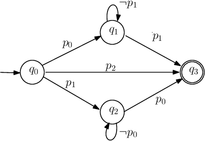
The DFA corresponding to the negation of the safe LTLF formula in (3) is shown in Figure 1(b). ∎
3 Barrier Certificate
We recall that a function is a supermartingale for system if
where the expectation is with respect to . This inequality requires that the expected value of does not increases as a function of time. To provide results for finite time horizon, we instead use a relaxation of supermartingale condition called c-martingale.
Definition 5
Function is a c-martingale for system if it satisfies
with being a non-negative constant.
We provide the following lemma and use it in the sequel. This lemma is a direct consequence of [13, Theorem 1] and is also utilized in [27, Theorem II.1].
Lemma 1
Let be a non-negative c-martingale for system . Then for any constant and any initial condition ,
| (4) |
Next theorem provides inequalities on a barrier certificate that gives an upper bound on reachability probabilities. This theorem is inspired by the result of [19, Theorem 15] that uses supermartingales for reachability analysis of continuous-time systems.
Theorem 3.1
Consider a discrete-time stochastic system and sets . Suppose there exist a non-negative function and constants and such that
| (5) | |||||
| (6) | |||||
| (7) |
Then the probability that the solution process of starts from initial state and reaches within time horizon is upper bounded by .
Proof
Theorem 3.1 enables us to formulate an optimization problem by minimizing the value of and in order to find an upper bound for finite-horizon reachability that is as tight as possible.
In the next section, we discuss how to translate LTLF verification problem into the computation of a collection of barrier certificates each satisfying inequalities of the form (5)-(7). Then we show in Section 5 how to use Theorem 3.1 to provide a lower bound on the probability of satisfying LTLF specifications over finite time horizon.
4 Decomposition into Sequential Reachability
Consider a DFA that accepts all finite words of length over that satisfy . Self-loops in the DFA play a central role in our decomposition. Let be a set of states of having self-loops, i.e., .
Accepting state run of . Sequence is called an accepting state run if , , and there exist a finite word such that for all . We denote the set of such finite words by and the set of accepting runs by . We also indicate the length of by , which is .
Let be the set of all finite accepting state runs of lengths less than or equal to excluding self-loops,
| (8) |
Computation of can be done efficiently using algorithms in graph theory by viewing as a directed graph. Consider as a directed graph with vertices and edges such that if and only if and there exist such that . From the construction of the graph, it is obvious that the finite path in the graph of length starting from vertices and ending at is an accepting state run q of without any self-loop thus belongs to . Then one can easily compute using variants of depth first search algorithm [21].
Decomposition into sequential reachability is performed as follows. For any , we define as a set of all state runs of length augmented with a horizon,
| (9) |
where the horizon is defined as for and otherwise.
Remark 3
Note that for . In fact, any accepting state run of length specifies a subset of the state space such that the system satisfies whenever it starts from that subset. This gives trivial zero probability for satisfying the specification, thus neglected in the sequel.
The computation of sets , , is illustrated in Algorithm 1 and demonstrated below for our demo example.
Example 2
(continued) For safe LTLF formula given in (3), Figure 1(b) shows a DFA that accepts all words that satisfy . From Figure 1(b), we get and . We consider traces of maximum length . The set of accepting state runs of lengths at most without self-loops is
The set of states with self-loops is . Then the sets for are as follows:
For every , the corresponding finite words are listed as follows:
∎
5 Computation of Probabilities Using Barrier Certificates
Having the set of state runs of length augmented with horizon, in this section, we provide a systematic approach to compute a lower bound on the probability that the solution process of satisfies . Given DFA , our approach relies on performing a reachability computation over each element of , , where reachability probability is upper bounded using barrier certificates.
Next theorem provides an upper bound on the probability that the solution process of the system satisfies the specification .
Theorem 5.1
For a given safe LTLF specification , let be a DFA corresponding to its negation, be the set of accepting state runs of length at most as defined in (8), and be the set of runs of length augmented with horizon as defined in (9). Then the probability that the system satisfies within time horizon is upper bounded by
| (10) |
where is the upper bound on the probability of the trajectories of starting from and reaching within time horizon computed via Theorem 3.1.
Proof
Consider an accepting run and set as defined in (9). For an element , the upper bound on the probability of trajectories of stating from and reaching within time horizon is given by . This follows from Theorem 3.1. Now the upper bound on the probability of the trace of the solution process reaching accepting state following trace corresponding to q is given by the product of the probability bounds corresponding to all elements and is given by
| (11) |
Note that, the way we computed time horizon , we always get the upper bound for the probabilities for all possible combinations of self-loops for accepting state runs of length less than or equal to . The upper bound on the probability that the solution processes of system violate can be computed by summing the probability bounds for all possible accepting runs as computed in (11) and is given by
∎
Theorem 5.1 enables us to decompose the computation into a collection of sequential reachability, compute bounds on the reachability probabilities using Theorem 3.1, and then combine the bounds in a sum-product expression.
Remark 4
Corollary 1
Given the result of Theorem 5.1, the probability that the trajectories of of length satisfies safe LTLF specification is lower-bounded by
5.1 Computation of barrier certificate
Proving existence of a barrier certificate, finding one, or showing that a given function is in fact a barrier certificate are in general hard problems. But if we restrict the class of systems and labeling functions, we can construct computationally efficient techniques for searching barrier certificates of specific forms. One technique is to use sum-of-squares (SOS) optimization [17], which relies on the fact that a polynomial is non-negative if it can be written as sum of squares of different polynomials. Therefore, we raise the following assumption.
Assumption 1
System has state set and its vector field is a polynomial function of state for any . Partition sets , , are bounded semi-algebraic sets, i.e., they can be represented by polynomial equalities and inequalities.
Under Assumption 1, we can formulate (5)-(7) as an SOS optimization problem to search for a polynomial-type barrier certificate and the tightest upper bound . The following lemma provides a set of sufficient conditions for the existence of such a barrier certificate required in Theorem 3.1, which can be solved as an SOS optimization.
Lemma 2
Suppose Assumption 1 holds and sets can be defined by vectors of polynomial inequalities , , and , where the inequalities are defined element-wise. Suppose there exists a sum-of-squares polynomial B(x), constants and , and vectors of sum-of-squares polynomials , , and of appropriate size such that following expressions are sum-of-squares polynomials
| (12) | |||
| (13) | |||
| (14) |
Proof
The proof is similar to that of Lemma 7 in [33] and is omitted due to lack of space. ∎
Remark 5
Assumption 1 is essential for applying the results of Lemma 2 to any LTLF specification. For a given specification, we can relax this assumption and allow some of the partition sets to be unbounded. For this, we require that the labels corresponding to unbounded partition sets should only appear either on self-loops or on accepting runs of length less than 3. For instance, Example 1 has an unbounded partition set and its corresponding label satisfies this requirement (see Figure 1), thus the results are still applicable for verifying the specification.
5.2 Computational complexity
Based on Lemma 2, a polynomial barrier certificate satisfying (5)-(7) and minimizing constants and can be automatically computed using SOSTOOLS [20] in conjunction with a semidefinite programming solver such as SeDuMi [28]. We refer the interested reader to [27] and [19] for more discussions. Note that the value of the upper bound of violating the property depends highly on the selection of degree of polynomials in Lemma 2.
From the construction of directed graph , explained in Section 4, the number of triplets and hence the number of barrier certificates needed to be computed are bounded by , where is the number of vertices in . Further, it is known [3] that is at most , where is the length of formula in terms of number of operations, but in practice, it is much smaller than this bound [11].
Computational complexity of finding polynomials in Lemma 2 depends on both the degree of polynomials appearing in (12)-(14) and the number of variables. It is shown that for fixed degrees the required computations grow polynomially with respect to the dimension [33]. Hence we expect that this technique is more scalable in comparison with the discretization-based approaches especially for large-scale systems.
6 Case Studies
In this section, we demonstrate the effectiveness of the proposed results on several case studies. We first showcase the results on the running example, which has nonlinear dynamics with additive noise. We then apply the technique to a ten-dimensional linear system with additive noise to show its scalability. The third case study is a three-dimensional nonlinear system with multiplicative noise.
6.1 Running example
To compute an upper bound on reachability probabilities corresponding to each element of in Theorem 5.1, we use Lemma 2 to formulate it as a SOS optimization problem to minimize values of and using bisection method. The optimization problem is solved using SOSTOOLS and SeDuMi, to obtain upper bounds in Theorem 5.1. The computed upper bounds on probabilities corresponding to the elements of , , , , , and are respectively , , , , and . Using Theorem 5.1, we get
Thus, a lower bound on the probability that trajectories of satisfy safe LTLF property (3) over time horizon is given by . The optimization finds polynomials of degree for , , , and . Hence barrier certificates are computed each with optimization coefficients, which takes minutes in total. For the sake of comparison, we provide a probabilistic guarantee from Monte-Carlo method using realizations, which results in the interval with confidence .
6.2 Thermal model of a ten-room building

Consider temperature evolution in a ten-room building shown schematically in Figure 2(a). We use this model to demonstrate the effectiveness of the results on large-dimensional state spaces. This model is adapted from [10] by discretizing it with sampling time minutes and without including heaters. The dynamics of are given as follows:
where , , denotes the temperature in each room, C is the ambient temperature, and , , and are heat exchange coefficients.
Noise terms , , are independent standard normal random variables. The state space of the system is . We consider regions of interest , , . The set of atomic propositions is given by with labeling function for all , . The objective is to compute a lower bound on the probability that the solution process of length satisfies the safe LTLF formula
| (15) |
The DFA corresponding to is shown in Figure 2(b). We use Algorithm 1 to get , , and . As described in Section 5, we compute two barrier certificates and SOS polynomials satisfying inequalities of Lemma 2. The lower bound is obtained using SOSTOOLS and SeDuMi for initial states starting from . The optimization finds , , , and as quadratic polynomials. Hence two barrier certificates are computed each with optimization coefficients, which takes minutes in total. For the sake of comparison, we provide a probabilistic guarantee from Monte-Carlo method using realizations, which results in the interval with confidence .

6.3 Lorenz model of a thermal convection loop
Our third case study is the Lorenz model of a thermal convection loop as used in [18] with multiplicative noise. The nonlinear dynamics of is given as
| (16) |
where , , and . Noise terms , , and are independent standard normal random variables. We refer the interested readers to [31] for a detailed treatment of the model. The state space of the system is . We define regions of interest as , , , and .
The set of atomic propositions is given by with labeling function for all , . We consider safe LTLF property and time horizon . The DFA corresponding to the negation of is shown in Figure 3. One can readily see that with . Thus, we need to compute only one barrier certificate. We use inequalities of Lemma 2 and find a barrier certificate that gives the lower bound . The optimization finds , , , and as polynomials of degree . Hence only one barrier certificate is computed with optimization coefficients, which takes minutes. For the sake of comparison, Monte-Carlo method results in the interval for the true probability with confidence using realizations.
Remark that current implementations of discretization-based approaches (e.g., [26]) are not directly applicable to the model in Subsection 6.1 and to the model (16) due to the multiplicative noise in the latter and unbounded state space of the former. Application of these techniques to the model in Subsection 6.2 will also be computationally much more expensive than our approach due to its exponential complexity as a function of state space dimension.
7 Conclusions
In this paper, we proposed a discretization-free approach for formal verification of discrete-time stochastic systems. The approach computes lower bounds on the probability of satisfying a specification encoded as safe LTL over finite traces. It is based on computation of barrier certificates and uses sum-of-squares optimization to find such bounds. From the implementation perspective, we plan to generalize our code and make it publicly available so that it can be applied to systems and specifications defined by users.
References
- [1] Abate, A., Katoen, J.P., Mereacre, A.: Quantitative automata model checking of autonomous stochastic hybrid systems. In: Proceedings of the 14th international conference on Hybrid systems: computation and control. pp. 83–92. ACM (2011)
- [2] Ayala, A.I.M., Andersson, S.B., Belta, C.: Probabilistic control from time-bounded temporal logic specifications in dynamic environments. In: 2012 IEEE International Conference on Robotics and Automation. pp. 4705–4710 (2012)
- [3] Baier, C., Katoen, J.P., Larsen, K.G.: Principles of model checking. MIT press (2008)
- [4] De Giacomo, G., Vardi, M.Y.: Linear temporal logic and linear dynamic logic on finite traces. In: International Joint Conference on Artificial Intelligence. vol. 13, pp. 854–860 (2013)
- [5] De Giacomo, G., Vardi, M.Y.: Synthesis for LTL and LDL on finite traces. In: International Joint Conference on Artificial Intelligence. vol. 15, pp. 1558–1564 (2015)
- [6] Dimitrova, R., Majumdar, R.: Deductive control synthesis for alternating-time logics. In: 2014 International Conference on Embedded Software (EMSOFT). pp. 1–10 (2014)
- [7] Duret-Lutz, A., Lewkowicz, A., Fauchille, A., Michaud, T., Renault, E., Xu, L.: Spot 2.0: A framework for LTL and omega -automata manipulation. In: International Symposium on Automated Technology for Verification and Analysis. pp. 122--129. Springer (2016)
- [8] Henriksen, J.G., Jensen, J., Jørgensen, M., Klarlund, N., Paige, R., Rauhe, T., Sandholm, A.: Mona: Monadic second-order logic in practice. In: International Workshop on Tools and Algorithms for the Construction and Analysis of Systems. pp. 89–110. Springer (1995)
- [9] Huang, C., Chen, X., Lin, W., Yang, Z., Li, X.: Probabilistic safety verification of stochastic hybrid systems using barrier certificates. ACM Transactions on Embedded Computing Systems 16(5s), 186 (2017)
- [10] Jagtap, P., Zamani, M.: QUEST: A tool for state-space quantization-free synthesis of symbolic controllers. In: International Conference on Quantitative Evaluation of Systems. pp. 309–313. Springer (2017), http://www.hcs.ei.tum.de/software/quest/
- [11] Klein, J., Baier, C.: Experiments with deterministic -automata for formulas of linear temporal logic. Theoretical Computer Science 363(2), 182–195 (2006)
- [12] Kupferman, O., Vardi, M.: Model checking of safety properties. In: International Conference on Computer Aided Verification. pp. 172–183. Springer (1999)
- [13] Kushner, H.J.: On the stability of stochastic dynamical systems. Proceedings of the National Academy of Sciences 53(1), 8–12 (1965)
- [14] Lahijanian, M., Andersson, S.B., Belta, C.: Formal verification and synthesis for discrete-time stochastic systems. IEEE Transactions on Automatic Control 60(8), 2031–2045 (2015)
- [15] Lavaei, A., Soudjani, S., Zamani, M.: From dissipativity theory to compositional construction of finite Markov decision processes. In: Hybrid Systems: Computation and Control (HSCC). pp. 21–30. ACM, New York, NY, USA (2018)
- [16] Maity, D., Baras, J.S.: Motion planning in dynamic environments with bounded time temporal logic specifications. In: 2015 23rd Mediterranean Conference on Control and Automation. pp. 940–946 (2015)
- [17] Parrilo, P.A.: Semidefinite programming relaxations for semialgebraic problems. Mathematical programming 96(2), 293–320 (2003)
- [18] Postoyan, R., Nesic, D.: Time-triggered control of nonlinear discrete-time systems. In: 2016 IEEE 55th Conference on Decision and Control. pp. 6814–6819 (2016)
- [19] Prajna, S., Jadbabaie, A., Pappas, G.J.: A framework for worst-case and stochastic safety verification using barrier certificates. IEEE Transactions on Automatic Control 52(8), 1415–1428 (2007)
- [20] Prajna, S., Papachristodoulou, A., Parrilo, P.A.: Introducing SOSTOOLS: a general purpose sum of squares programming solver. In: Proceedings of the 41st IEEE Conference on Decision and Control. vol. 1, pp. 741–746 (2002), http://www.cds.caltech.edu/sostools/
- [21] Russell, S.J., Norvig, P.: Artificial Intelligence: A Modern Approach. Pearson Education, 2 edn. (2003)
- [22] Saha, I., Ramaithitima, R., Kumar, V., Pappas, G.J., Seshia, S.A.: Automated composition of motion primitives for multi-robot systems from safe LTL specifications. In: 2014 IEEE/RSJ International Conference on Intelligent Robots and Systems. pp. 1525–1532 (2014)
- [23] Soudjani, S., Abate, A.: Precise approximations of the probability distribution of a Markov process in time: an application to probabilistic invariance. In: TACAS, LNCS, vol. 8413, pp. 547–561. Springer (2014)
- [24] Soudjani, S., Abate, A., Majumdar, R.: Dynamic Bayesian networks as formal abstractions of structured stochastic processes. In: 26th International Conference on Concurrency Theory. pp. 1–14. Dagstuhl Publishing, Madrid, Spain (2015)
- [25] Soudjani, S., Abate, A.: Adaptive and sequential gridding procedures for the abstraction and verification of stochastic processes. SIAM Journal on Applied Dynamical Systems 12(2), 921–956 (2013)
- [26] Soudjani, S., Gevaerts, C., Abate, A.: FAUST2: Formal Abstractions of Uncountable-STate STochastic processes. In: Baier, C., Tinelli, C. (eds.) Tools and Algorithms for the Construction and Analysis of Systems. pp. 272–286. Springer Berlin Heidelberg, Berlin, Heidelberg (2015)
- [27] Steinhardt, J., Tedrake, R.: Finite-time regional verification of stochastic non-linear systems. The International Journal of Robotics Research 31(7), 901–923 (2012)
- [28] Sturm, J.F.: Using SeDuMi 1.02, a MATLAB toolbox for optimization over symmetric cones. Optimization methods and software 11(1-4), 625–653 (1999), http://sedumi.ie.lehigh.edu/
- [29] Tabuada, P.: Verification and control of hybrid systems: a symbolic approach. Springer Science & Business Media (2009)
- [30] Tkachev, I., Abate, A.: Formula-free finite abstractions for linear temporal verification of stochastic hybrid systems. In: Proceedings of the 16th international conference on Hybrid systems: computation and control. pp. 283–292. ACM (2013)
- [31] Vincent, T.L., Yu, J.: Control of a chaotic system. Dynamics and Control 1(1), 35–52 (1991)
- [32] Wisniewski, R., Bujorianu, M.L.: Stochastic safety analysis of stochastic hybrid systems. In: 2017 IEEE 56th Annual Conference on Decision and Control. pp. 2390–2395 (2017)
- [33] Wongpiromsarn, T., Topcu, U., Lamperski, A.: Automata theory meets barrier certificates: Temporal logic verification of nonlinear systems. IEEE Transactions on Automatic Control 61(11), 3344–3355 (2016)