Clock Constraint Specification Language (Ccsl) [26, 6] is a UML profile for modeling and analysis of real-time systems (MARTE) [7, 25]. In Ccsl, a clock represents a sequence of (possibly infinite) instants. An event is a clock and the occurrences of an event correspond to a set of ticks of the clock. Ccsl provides a set of clock constraints that specifies evolution of clocks’ ticks. The physical time is represented by a dense clock with a base unit. A dense clock can be discretized into a discrete/logical clock. $idealClock$ is a predefined dense clock whose unit is second. We define a universal clock $ms$ based on $idealClock$: $ms$ = $idealClock$ discretizedBy 0.001. $ms$ representing a periodic clock that ticks every 1 millisecond in this paper. A step is a tick of the universal clock. Hence the length of one step is 1 millisecond.

UPPAAL-SMC performs the probabilistic analysis of properties by monitoring simulations of complex hybrid systems in a given stochastic environment and using results from the statistics to determine whether the system satisfies the property with some degree of confidence. Its clocks evolve with various rates, which are specified with ordinary differential equations (ODE). Uppaal-SMC provides a number of queries related to the stochastic interpretation of Timed Automata (STA) [12] and they are as follows, where $N$ and $bound$ indicate the number of simulations to be performed and the time bound on the simulations respectively:

1. 1.

   Probability Estimation estimates the probability of a requirement property $\phi$ being satisfied for a given STA model within the time bound: $Pr[bound]\ \phi$.

2. 2.

   Hypothesis Testing checks if the probability of $\phi$ being satisfied is larger than or equal to a certain probability $P_{0}$: $Pr[bound]\ \phi\ \geqslant\ P_{0}$.

3. 3.

   Probability Comparison compares the probabilities of two properties being satisfied in certain time bounds: $Pr[bound_{1}]$ $\phi_{1}$ $\geqslant$ $Pr[bound_{2}]$ $\phi_{2}$.

4. 4.

   Expected Value evaluates the minimal or maximal value of a clock or an integer value while Uppaal-SMC checks the STA model: $E[bound;N](min:\phi)$ or $E[bound;N](max:\phi)$.

5. 5.

   Simulations: Uppaal-SMC runs $N$ simulations on the STA model and monitors $k$ (state-based) properties/expressions $\phi_{1},...,\phi_{k}$ along the simulations within simulation bound $bound$: $simulate$ $N$ $[\leqslant$ $bound]\{\phi_{1},...,\phi_{k}\}$.

R1. The camera must capture an image every 50ms. In other words, a Periodic acquisition of Camera must be carried out every 50ms.

R2. The captured image must be recognized by an AV every 200ms, which can be interpreted as a Periodic constraint on SignRecognition $f_{p}$.

R3. The obstacle will be detected by vehicle every 40ms, i.e., a Periodic timing constraint should be applied on the obstacle input port of Controller.

R4. The speed of the vehicle should be updated periodically with the period as 30ms, i.e., a Periodic timing constraint should be applied on the speed input port of Controller.

R5. The detected image should be computed within [100, 150]ms in order to generate the desired sign type, the SignRecognition must complete its execution within [100, 150]ms.

R6. After the Camera is triggered, the captured image should be sent out from Camera within 20 – 30ms, i.e., the execution time of Camera should be between 20 and 30ms.

R7. After an obstacle is detected, the Controller should send out a request to brake the vehicle within 100 – 150ms, i.e., the execution time for Controller should be in the range [100, 150]ms.

R8. After the command/request from controller is arrived at VehicleDynamic, the speed should be updated within 50 – 100ms. That is, the Execution timing constraint applied on VehicleDynamic is 50 – 100ms.

R9. If the mode of AV switches to “emergency stop” due to the certain obstacle, it should not revert back to “automatic running” mode within a specific time period. That is interpreted as a Sporadic constraint, i.e., the mode of AV is changed to “stop” because of the encounter of obstacle, it should not revert back to “run” mode within 500ms.

R10. If the mode of AV switches to “emergency stop” due to the certain obstacle, it should not revert back to “accelerate ” mode within a specific time period. That is interpreted as a Sporadic constraint, i.e., the mode of AV is changed to “stop” because of the encounter of obstacle, it should not revert back to “accelerate” mode within 500ms.

R11. If the mode of AV switches to “emergency stop” due to the certain obstacle, it should not revert back to “turn left” mode within a specific time period. That is interpreted as a Sporadic constraint, i.e., the mode of AV is changed to “stop” because of the encounter of obstacle, it should not revert back to “turn left” mode within 500ms.

R12. If the mode of AV switches to “emergency stop” due to the certain obstacle, it should not revert back to “turn right” mode within a specific time period. That is interpreted as a Sporadic constraint, i.e., the mode of AV is changed to “stop” because of the encounter of obstacle, it should not revert back to “turn right” mode within 500ms.

R13. The required environmental information should arrive to the controller within 40ms. That is input signals (speed, signType, direct, gear and torque ports) must be detected by Controller within a given time window, i.e., the tolerated maximum constraint is 40ms.

R14. After the execution of Controller is finished, all the requests of controller should be updated within 30ms. That is output signals (on reqTorq, reqDirect, reqGear, reqBrake ports) must be sent within a given time window, i.e., the tolerated maximum constraint is 30ms.

R15. The requests from the controller should be arrived to VehicleDynamic within 30ms. That is input signals (reqTorq, reqDirect, reqGear, reqBrake) must be detected by VehicleDynamic within a given time window, i.e., the tolerated maximum constraint is 30ms.

R16. After execution of VehicleDynamic is finished, the information of vehicle should be updated within 40ms, i.e., the Synchronization applied on the output ports (speed, direct, gear, torque) is 40ms.

R17. When a traffic sign is recognized, the speed of AV should be updated within [150, 250]ms. An End-to-End constraint on Controller and VehicleDynamic, i.e., the time interval measured from the input arrival of Controller to the instant at which the corresponding output is sent out from VehicleDynamic must be within [150, 250]ms.

R18. After the camera is triggered to capture the image, the computation of the traffic sign should be finished within [120, 180]ms, i.e., the End-to-End timing constraint applied on Camera and SignRecognition should be between 120ms and 180ms.

R19. The time interval measured from the instant at which the camera captures an image of traffic sign, to the instant at which the status of AV (i.e., speed, direction) is updated, should be within [270, 430]ms. That is, End-to-End timing constraint applied on Camera and VehicleDynamic should be between 270 and 430ms.

R20. When a left turn sign is recognized, the vehicle should turn towards left within 500ms, which can be interpreted as an End-to-End timing constraint applied on the event DetectLeftSign and StartTurnLeft.

R21. When a right turn sign is recognized, the vehicle should turn towards right within 500ms, which can be interpreted as an End-to-End timing constraint applied on the event DetectRightSign and StartTurnRight.

R22. When a stop sign is recognized, the vehicle should start to brake within 200ms, which can be interpreted as an End-to-End timing constraint applied on the event DetectStopSign and StartBrake.

R23. When a stop sign is recognized, the vehicle should be stop completely within 3000ms, which can be interpreted as an End-to-End timing constraint applied on the event DetectStopSign and Stop.

R24. The execution time interval from Controller to VehicleDynamic should be less than or equal to the sum of the worst case execution time interval of each $f_{p}$.

R25. The execution time interval from Camera to SignRecognition should be less than or equal to the sum of the worst case execution time interval of each $f_{p}$.

R26. The execution time interval from Camera to VehicleDynamic should be less than or equal to the sum of the worst case execution time interval of each $f_{p}$.

R27. While AV turns left, the “turning right” mode should not be activated. The events of turning left and right considered as exclusive and specified as an Exclusion constraint.

R28. While AV is braking, the “accelerate” mode should not be activated. The events of braking and accelerating are considered as exclusive and specified as an Exclusion constraint.

R29. When AV is in the emergency mode because of the obstacle occurrence, “turn left” mode must not be activated, i.e., the events of handling emergency and turning left are exclusive and specified as a Exclusion constraint.

R30. When AV is in the emergency mode because of the encounter of an obstacle, “turn right” mode must not be activated, i.e., the events of handling emergency and turning right are exclusive and specified as an Exclusion constraint.

R31. When AV is in the emergency mode because of the encounter of an obstacle, “accelerate” mode must not be activated, i.e., the events of handling emergency and accelerating are exclusive and specified as an Exclusion constraint.

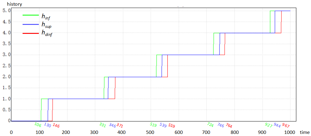
Fig. 4.1 presents a run $R$ consisting of $10$ steps and three clocks $c1$, $c2$ and $c3$. The ticks of the three clocks along with steps are shown as “cross” symbols (x). For instance, $c1$, $c2$ and $c3$ tick at the first step, hence $R(1)$ = {$c1,\ c2,\ c3$}.

A run $R_{j}$ satisfies the subclock relation between $c1$ and $c2$ “if $c1$ ticks, $c2$ must tick” holds at every step $i$ in $R_{j}$, s.t., $(R_{j}\models c1{\color[rgb]{1,0,0}\subseteq}c2)\Longleftrightarrow(\forall i$ $0\leqslant i\leqslant n,\ c1\in{R}(i)\implies c2\in{R}(i))$. “$R_{j}\models c1{\color[rgb]{1,0,0}\subseteq}c2$” returns 1 if $R_{j}$ satisfies $c1{\color[rgb]{1,0,0}\subseteq}c2$, otherwise it returns 0.

A run, $R_{j}$ satisfies the coincidence relation on $c1$ and $c2$ if the assertion holds: $\forall i$, $0\leqslant i\leqslant n$, $(c1\in{R}(i)\implies c2\in{R}(i))\wedge\ (c2\in{R}(i)\implies c1\in{R}(i))$. In other words, the satisfaction of coincidence relation is established when the two conditions “if $c1$ ticks, $c2$ must tick” and “if $c2$ ticks, $c1$ must tick” hold at every step.

A run, $R_{j}$, satisfies the exclusion relation on $c1$ and $c2$ if $\forall i$, $0\leqslant i\leqslant n$, $(c1\in{R}(i)\implies c2\notin{R}(i))\wedge\ (c2\in{R}(i)\implies c1\notin{R}(i))$, i.e., for every step, if $c1$ ticks, $c2$ must not tick and vice versa.

A run $R_{j}$ satisfies the causality relation on $c1$ and $c2$ if the condition holds: $\forall i$, $0\leqslant i\leqslant n$, $H^{c1}_{R}(i)\geqslant H^{c2}_{R}(i)$. A tick of $c1$ satisfies causality relation if $c2$ does not occur prior to $c1$, i.e., the history of $c2$ is less than or equal to the history of $c1$ at the current step $i$.

A run $R_{j}$ satisfies the precedence relation if the condition (expressed as $(1)\land(2)$) holds: $\forall i$, $0\leqslant i\leqslant n$,

$$\underbrace{(H^{c1}_{R}(i)\geqslant H^{c2}_{R}(i))}_{\text{(1)}}\wedge\underbrace{(H^{c2}_{R}(i)=H^{c1}_{R}(i))\implies(c2\notin\ {R}(i))}_{\text{(2)}}$$

(1) The history of $c1$ is greater than or equal to the history of $c2$; (2) $c1$ and $c2$ must not be coincident, i.e., when the history of $c1$ and $c2$ are equal, $c2$ must not tick.

Periodic timing constraints (R1 – R4) can be specified using periodicOn expression and probabilistic coincident relation. R1 states that the camera must be triggered periodically with a period 50ms. We first construct a periodic clock $prd\_50$ which ticks after every $50$ ticks of $ms$ (the universal clock). Then the property that the periodic timing constraint is satisfied with probability no less than the threshold $p$ can be interpreted as the probabilistic coincidence relation between $cmrTrig$ (the event that Camera $f_{p}$ being triggered) and $prd\_50$. The corresponding specification is given below, where $\triangleq$ means “is defined as”:

$$prd\_50\ \triangleq\ \texttt{periodicOn}\ ms\ \texttt{period}\ 50$$

(5.1)

$${cmrTrig}\ {\color[rgb]{1,0,0}\equiv_{p}}\ prd\_50$$

(5.2)

By combining (1) and (2), we can obtain the the specification of R1:

$${cmrTrig}\ {\color[rgb]{1,0,0}\equiv_{p}}\ \{\texttt{periodicOn}\ ms\ \texttt{period}\ 50\}$$

(5.3)

In similar, the Ccsl/PrCcsl specification of R2 – R4 can be derived:

$$\textbf{R2}:\ {signTrig}\ {\color[rgb]{1,0,0}\equiv_{p}}\ \{\texttt{periodicOn}\ ms\ \texttt{period}\ 200\}$$

(5.4)

$$\textbf{R3}:\ {obsDetect}\ {\color[rgb]{1,0,0}\equiv_{p}}\ \{\texttt{periodicOn}\ ms\ \texttt{period}\ 40\}$$

(5.5)

$$\textbf{R4}:\ {spUpdate}\ {\color[rgb]{1,0,0}\equiv_{p}}\ \{\texttt{periodicOn}\ ms\ \texttt{period}\ 30\}$$

(5.6)

where $signTrig$ is the event/clock that SignRecognition $f_{p}$ is triggered, $obsDetect$ represents the event that the object detection is activated by the vehicle and $spUpdate$ denotes the event that the speed is updated (i.e., recieved by Controller) from the environment.

Since the $period$ attribute of the Periodic timing constraint R2 is 200ms, which is an integral multiple of the $period$ of R1, R2 can be interpreted as a subclock relation, i.e., the event $signTrig$ should be a subclock of $cmrTrig$. The specification is given below:

$$\ {signTrig}\ {\color[rgb]{1,0,0}\subseteq_{p}}\ cmrTrig$$

(5.7)

Execution timing constraints (R5 – R8) can be specified using delayFor expression and probabilistic causality relation. To specify R5, which states that the SignRecognition $f_{p}$ must finish execution within [100, 150]ms, i.e., the interval measured from the input event of the $f_{p}$ (i.e., the event that the image is received by the $f_{p}$, denoted $imIn$) to the output event of the $f_{p}$ (denoted $imIn$) must have a minimum value 100 and a maximum value 150. We divide this property into two subproperties: R5(1) The time duration between $imIn$ and $signOut$ should be greater than 100ms. R5(2) The time duration between $imIn$ and $signOut$ should be less than 150ms. To specify property R5(1), we first construct a new clock $imIn\_dly100$ by delaying $imIn$ (the input event of SignRecognition) for 100ms. To check whether R5(1) is satisfied within a probability threshold is to verify whether the probabilistic causality between $imIn\_dly100$ and $signOut$ is valid. The specification of R5(1) is given below:

$$imIn\_dly100\ \triangleq\ imIn\ \texttt{delayFor}\ 100\ \texttt{on}\ ms$$

(5.8)

$${imIn\_dly100}\ {\color[rgb]{1,0,0}\preceq_{p}}\ signOut$$

(5.9)

By combining (7) and (8), we can obtain the the specification of R5(1):

$$\{{imIn}\ \texttt{delayFor}\ 100\ \texttt{on}\ ms\}\ {\color[rgb]{1,0,0}\preceq_{p}}\ signOut$$

(5.10)

Sporadic timing constraints (R9 – R12) can be specified using delayFor expression and probabilistic precedence relation. R9 states that there should be a minimum delay between the event $veRun$ (the event that the vehicle is in the “run” mode) and the event $obstc$ (the event that the vehicle detects an obstacle), which is specified as 500ms. To specify R9, we first build a new clock $obstc\_dly500$ by delaying $obstc$ for 500 ticks of $ms$. We then check the probabilistic precedence relation between $obst\_dly500$ and $veRun$:

$$obstc\_dly500\ \triangleq\ obstc\ \texttt{delayFor}\ 500\ \texttt{on}\ ms$$

(5.17)

$${obstc\_dly500}\ {\color[rgb]{1,0,0}\prec_{p}}\ veRun$$

(5.18)

By combining (16) and (17), we can obtain the the specification of R9:

$$\{obstc\ \texttt{delayFor}\ 500\ \texttt{on}\ ms\}\ {\color[rgb]{1,0,0}\prec_{p}}\ veRun$$

(5.19)

Analogously, the Ccsl/PrCcsl specification of R10 – R12 can be derived:

$$\textbf{R10}:\ \{obstc\ \texttt{delayFor}\ 500\ \texttt{on}\ ms\}\ {\color[rgb]{1,0,0}\prec_{p}}\ veAcc$$

(5.20)

$$\textbf{R11}:\ \{obstc\ \texttt{delayFor}\ 500\ \texttt{on}\ ms\}\ {\color[rgb]{1,0,0}\prec_{p}}\ tLeft$$

(5.21)

$$\textbf{R12}:\ \{obstc\ \texttt{delayFor}\ 500\ \texttt{on}\ ms\}\ {\color[rgb]{1,0,0}\prec_{p}}\ tRight$$

(5.22)

where $veAcc$ is the event/clock that the vehicle is accelerating. $tLeft$ and $tRight$ represent the event that the vehicle transits from the “emergency stop” mode to “turn left” and “turn right” mode respectively.

Synchronization timing constraints (R13 – R16) can be specified using infimum and supremum expression, together with probabilistic precedence relation. R13 states that the five input events must be detected by Controller within the maximum tolerated time, given as 40ms. The synchronization timing constraint can be interpreted as: the time interval between the earliest/fastest and the latest/slowest event among the five input events, i.e., speed, signType, direct, gear and torque, must not exceed 40ms. To specify the constraints, infimum is utilized to express the fastest event (denoted $inf_{ctrlIn}$) while supremum is utilized to specify the slowest event $sup_{ctrlIn}$. $sup_{ctrlIn}$ and $inf_{ctrlIn}$ are defined as:

$$sup_{ctrl}\ \triangleq\ {{\texttt{Sup}}}({{\texttt{Sup}}}({\emph{speed}},\ {\emph{signType}}),\ {{\texttt{Sup}}}({\texttt{Sup}}({\emph{direct}},\ {\emph{gear}}),\ {\emph{torque}}))$$

(5.23)

$$inf_{ctrl}\ \triangleq\ {\texttt{Inf}}({\texttt{Inf}}({\emph{speed}},\ {\emph{signType}}),\ {\texttt{Inf}}({\texttt{Inf}}({\emph{direct}},\ {\emph{gear}}),\ {\emph{torque}}))$$

(5.24)

where Inf($c1$, $c2$) (resp. Sup($c1$, $c2$)) is the infimum (resp. supremum) operator returns the slowest clock faster than $c1$ and $c2$. Afterwards, we construct a new clock $inf_{ctrlIn}\_dly40$ that is the $inf_{ctrlIn}$ delayed for 40 ticks of $ms$, which is defined as:

$$inf_{ctrlIn}\_dly40\ \triangleq\ inf_{ctrl}\ \texttt{delayFor}\ 40\ \texttt{on}\ ms$$

(5.25)

Therefore, the synchronization constraint R13 can be represented as the proba-
bilistic causality relation between $sup_{ctrlIn}$ and $inf_{ctrlIn}\_dly40$, given as the Ccsl/PrCcsl expression below:

$$sup_{ctrlIn}\ {\color[rgb]{1,0,0}\preceq_{p}}\ {inf_{ctrlIn}\_dly40}$$

(5.26)

By combining (24) and (25), we can obtain the the specification of R13:

$$sup_{ctrlIn}\ {\color[rgb]{1,0,0}\preceq_{p}}\ \{inf_{ctrlIn}\ \texttt{delayFor}\ 40\ \texttt{on}\ ms\}$$

(5.27)

In similar, the Ccsl/PrCcsl specification of R14 – R16 can be derived. For R14, we first construct the clocks that represent the fastest and slowest output event/clock among the four output events of Controller $f_{p}$, i.e., reqTorq, reqDirect, reqGear and reqBrake. Then the property that the synchronization constraint is satisfied with a probability greater than or equal to $p$ can be interpreted as a probabilistic causality relation:

$$\begin{split}\textbf{R14}:sup_{ctrlOut}\ \triangleq\ \texttt{Sup}(\texttt{Sup}(\emph{reqTorq},\ \emph{reqDirect}),\ \texttt{Sup}(\emph{reqGear},\ \emph{reqBrake}))\\ inf_{ctrlOut}\ \triangleq\ \texttt{Inf}(\texttt{Inf}(\emph{reqTorq},\ \emph{reqDirect}),\ \texttt{Inf}(\emph{reqGear},\ \emph{reqBrake}))\\ sup_{ctrlOut}\ {\color[rgb]{1,0,0}\preceq_{p}}\ \{inf_{ctrlOut}\ \texttt{delayFor}\ 30\ \texttt{on}\ ms\}\end{split}$$

(5.28)

For R15, we first construct the fastest and slowest input event/clock among the four input events of VehicleDynamic , i.e., reqTorq, reqDirect, reqGear and reqBrake. Then the property that the synchronization constraint is satisfied with a probability greater than or equal to $p$ can be interpreted as a probabilistic causality relation:

$$\begin{split}\textbf{R15}:sup_{vdIn}\ \triangleq\ \texttt{Sup}(\texttt{Sup}(\emph{reqTorq},\ \emph{reqDirect}),\ \texttt{Sup}(\emph{reqGear},\ \emph{reqBrake}))\\ inf_{vdIn}\ \triangleq\ \texttt{Inf}(\texttt{Inf}(\emph{reqTorq},\ \emph{reqDirect}),\ \texttt{Inf}(\emph{reqGear},\ \emph{reqBrake}))\\ sup_{vdIn}\ {\color[rgb]{1,0,0}\preceq_{p}}\ \{inf_{vdIn}\ \texttt{delayFor}\ 40\ \texttt{on}\ ms\}\end{split}$$

(5.29)

For R16, we first construct the fastest and slowest output event/clock among the four output events of VehicleDynamic , i.e., speed, direct, torque and gear. Then the property that the synchronization constraint is satisfied with a probability greater than or equal to $p$ can be interpreted as a probabilistic causality relation:

$$\begin{split}\textbf{R16}:sup_{vdOut}\ \triangleq\ \texttt{Sup}(\texttt{Sup}(speed,\ direct),\ \texttt{Sup}(gear,\ torque))\\ inf_{vdOut}\ \triangleq\ \texttt{Inf}(\texttt{Inf}(speed,\ direct),\ \texttt{Inf}(gear,\ torque))\\ sup_{vdOut}\ {\color[rgb]{1,0,0}\preceq_{p}}\ \{inf_{vdOut}\ \texttt{delayFor}\ 40\ \texttt{on}\ ms\}\end{split}$$

(5.30)

End-to-End timing constraints (R17 – R23) can be specified using delayFor expression and probabilistic precedence relation. To specify R17, which limits that the time duration measured from the instant of the occurrence of the event that Controller $f_{p}$ receive the traffic sign type information (denoted as $signIn$), to the occurrence of event that the speed is sent out from the output port of VehicleDynamic $f_{p}$ (denoted as $spOut$) should be between 150 and 250ms. We divide this property into two subproperties: R17(1). The time duration between $signIn$ and $spOut$ should be more than 150ms. R17(2). The time duration between $signIn$ and $spOut$ should be less than 250ms. To specify property R17(1), we first construct a new clock $signIn\_dly150$ by delaying $signIn$ for 150ms. To check whether R17(1) is satisfied within a probability threshold $p$ is to verify whether the probabilistic precedence between $signIn\_dly150$ and $spOut$ is valid. The specification of R17(1) is given below:

$$signIn\_dly150\ \triangleq\ signIn\ \texttt{delayFor}\ 150\ \texttt{on}\ ms$$

(5.31)

$${signIn\_dly150}\ {\color[rgb]{1,0,0}\prec_{p}}\ spOut$$

(5.32)

By combining (30) and (31), we can obtain the the specification of R17(1):

$$\{{signIn}\ \texttt{delayFor}\ 150\ \texttt{on}\ ms\}\ {\color[rgb]{1,0,0}\prec_{p}}\ spOut$$

(5.33)

Similarly, to specify property R17(2), a new clock $signIn\_dly250$ is generated by delaying $signIn$ for 250 ticks on $ms$. Afterwards, the property that R17(2) is satisfied with a probability greater than or equal to $p$ relies on whether the probabilistic precedence relation is satisfied. The specification is illustrated as follows:

$$signIn\_dly250\ \triangleq\ signIn\ \texttt{delayFor}\ 250\ \texttt{on}\ ms$$

(5.34)

$${spOut}\ {\color[rgb]{1,0,0}\prec_{p}}\ signIn\_dly250$$

(5.35)

By combining (33) and (34), we can obtain the the specification of R17(2):

$${spOut}\ {\color[rgb]{1,0,0}\prec_{p}}\ \{{signIn}\ \texttt{delayFor}\ 250\ \texttt{on}\ ms\}$$

(5.36)

In similar, the Ccsl/PrCcsl specification of R18 – R23 can be derived:

$$\begin{split}\textbf{R18}:\ \{{cmrTrig}\ \texttt{delayFor}\ 120\ \texttt{on}\ ms\}\ {\color[rgb]{1,0,0}\prec_{p}}\ signOut\\ {signOut}\ {\color[rgb]{1,0,0}\prec_{p}}\ \{{cmrTrig}\ \texttt{delayFor}\ 180\ \texttt{on}\ ms\}\end{split}$$

(5.37)

$$\begin{split}\textbf{R19}:\ \{{cmrTrig}\ \texttt{delayFor}\ 270\ \texttt{on}\ ms\}\ {\color[rgb]{1,0,0}\prec_{p}}\ spOut\\ {spOut}\ {\color[rgb]{1,0,0}\prec_{p}}\ \{{cmrTrig}\ \texttt{delayFor}\ 430\ \texttt{on}\ ms\}\end{split}$$

(5.38)

$$\textbf{R20}:\ \{{startTurnLeft}\ {\color[rgb]{1,0,0}\prec_{p}}\ DetectLeftSign\ \texttt{delayFor}\ 500\ \texttt{on}\ ms\}$$

(5.39)

$$\textbf{R21}:\ \{{startTurnRight}\ {\color[rgb]{1,0,0}\prec_{p}}\ DetectRightSign\ \texttt{delayFor}\ 500\ \texttt{on}\ ms\}$$

(5.40)

$$\textbf{R22}:\ \{{startBrake}\ {\color[rgb]{1,0,0}\prec_{p}}\ DetectStopSign\ \texttt{delayFor}\ 500\ \texttt{on}\ ms\}$$

(5.41)

$$\textbf{R23}:\ \{{Stop}\ {\color[rgb]{1,0,0}\prec_{p}}\ DetectStopSign\ \texttt{delayFor}\ 3000\ \texttt{on}\ ms\}$$

(5.42)

Comparison timing constraints (R24 – R26) can be specified using delayFor expression and probabilistic causality relation. R24 states that the execution time interval from Controller to VehicleDynamic should be less than or equal to the sum of the worst case execution time of Controller and VehicleDynamic, denoted as W_ctrl and W_vd respectively. To specify comparison constraint, we first construct a new clock $signIn\_dly250$ by delaying $signIn$ for 250 ticks of $ms$. Afterwards, we generate another new clock $signIn\_dlysw$ that is the $signIn$ clock delayed for sum of the worst case execution time of the two $f_{p}$s. The specification is illustrated as follows:

$$signIn\_dly250\ \triangleq\ signIn\ \texttt{delayFor}\ 250\ \texttt{on}\ ms$$

(5.43)

$$signIn\_dlysw\ \triangleq\ signIn\ \texttt{delayFor}\ (W_{ctrl}+W_{vd})\ \texttt{on}\ ms$$

(5.44)

References

- [1] Automotive open system architecture. https://www.autosar.org/
- [2] UPPAAL-SMC. http://people.cs.aau.dk/~adavid/smc/
- [3] IEC 61508: Functional safety of electrical electronic programmable electronic safety related systems. International Organization for Standardization, Geneva (2010)
- [4] ISO 26262-6: Road vehicles functional safety part 6. Product development at the software level. International Organization for Standardization, Geneva (2011)
- [5] MAENAD. http://www.maenad.eu/ (2011)
- [6] André, C.: Syntax and semantics of the clock constraint specification language (CCSL). Ph.D. thesis, INRIA (2009)
- [7] André, C., Mallet, F.: Clock constraints in UML/MARTE CCSL. HAL - INRIA (2008)
- [8] Bernat, G., Burns, A., Llamosi, A.: Weakly hard real-time systems. Transactions on Computers 50(4), 308 – 321 (2001)
- [9] Blom, H., Feng, L., Lönn, H., Nordlander, J., Kuntz, S., Lisper, B., Quinton, S., Hanke, M., Peraldi-Frati, M.A., Goknil, A., Deantoni, J., Defo, G.B., Klobedanz, K., Özhan, M., Honcharova, O.: TIMMO-2-USE Timing Model, Tools, Algorithms, Languages, Methodology, Use Cases. Tech. rep., TIMMO-2-USE (2012)
- [10] Bulychev, P., David, A., Larsen, K.G., Mikučionis, M., Poulsen, D.B., Legay, A., Wang, Z.: UPPAAL-SMC: Statistical model checking for priced timed automata. In: QAPL. pp. 1–16. EPTCS (2012)
- [11] David, A., Du, D., Larsen, K.G., Legay, A., Mikučionis, M., Poulsen, D.B., Sedwards, S.: Statistical model checking for stochastic hybrid systems. In: HSB. pp. 122 – 136. EPTCS (2012)
- [12] David, A., Larsen, K.G., Legay, A., Mikučionis, M., Poulsen, D.B.: UPPAAL-SMC tutorial. STTT 17(4), 397 – 415 (2015)
- [13] Du, D., Huang, P., Jiang, K., Mallet, F., Yang, M.: MARTE/pCCSL: Modeling and refining stochastic behaviors of CPSs with probabilistic logical clocks. In: FACS. pp. 111 – 133. Springer (2016)
- [14] EAST-ADL Consortium: EAST-ADL domain model specification v2.1.9. Tech. rep., MAENAD European Project (2011)
- [15] Goknil, A., Suryadevara, J., Peraldi-Frati, M.A., Mallet, F.: Analysis support for TADL2 timing constraints on EAST-ADL models. In: ECSA. pp. 89 – 105. Springer (2013)
- [16] Kang, E.Y., Chen, J., Ke, L., Chen, S.: Statistical analysis of energy-aware real-time automotive systems in EAST-ADL/Stateflow. In: ICIEA. pp. 1328 – 1333. IEEE (2016)
- [17] Kang, E.Y., Enoiu, E.P., Marinescu, R., Seceleanu, C., Schobbens, P.Y., Pettersson, P.: A methodology for formal analysis and verification of EAST-ADL models. Reliability Engineering & System Safety 120(12), 127–138 (2013)
- [18] Kang, E.Y., Huang, L., Mu, D.: Formal verification of energy and timed requirements for a cooperative automotive system. In: SAC. pp. 1492 – 1499. ACM (2018)
- [19] Kang, E.Y., Ke, L., Hua, M.Z., Wang, Y.X.: Verifying automotive systems in EAST-ADL/Stateflow using UPPAAL. In: APSEC. pp. 143 – 150. IEEE (2015)
- [20] Kang, E.Y., Mu, D., Huang, L., Lan, Q.: Model-based analysis of timing and energy constraints in an autonomous vehicle system. In: QRS. pp. 525 – 532. IEEE (2017)
- [21] Kang, E.Y., Mu, D., Huang, L., Lan, Q.: Verification and validation of a cyber-physical system in the automotive domain. In: QRS. pp. 326 – 333. IEEE (2017)
- [22] Kang, E.Y., Schobbens, P.Y.: Schedulability analysis support for automotive systems: from requirement to implementation. In: SAC. pp. 1080 – 1085. ACM (2014)
- [23] Kang, E.Y., Schobbens, P.Y., Pettersson, P.: Verifying functional behaviors of automotive products in EAST-ADL2 using UPPAAL-PORT. In: SAFECOMP. pp. 243 – 256. Springer (2011)
- [24] Legay, A., Viswanathan, M.: Statistical model checking: challenges and perspectives. STTT 17(4), 369 – 376 (2015)
- [25] Mallet, F., Peraldi-Frati, M.A., Andre, C.: MARTE CCSL to execute EAST-ADL timing requirements. In: ISORC. pp. 249 – 253. IEEE (2009)
- [26] Mallet, F., De Simone, R.: Correctness issues on MARTE/CCSL constraints. Science of Computer Programming 106, 78 – 92 (2015)
- [27] Marinescu, R., Kaijser, H., Mikučionis, M., Seceleanu, C., Lönn, H., David, A.: Analyzing industrial architectural models by simulation and model-checking. In: FTSCS. pp. 189 – 205. Springer (2014)
- [28] Nicolau, G.B.: Specification and analysis of weakly hard real-time systems. Transactions on Computers pp. 308 – 321 (1988)
- [29] Object Management Group: UML profile for MARTE: Modeling and analysis of real-time embedded systems (2015)
- [30] Qureshi, T.N., Chen, D.J., Persson, M., Törngren, M.: Towards the integration of UPPAAL for formal verification of EAST-ADL timing constraint specification. In: TiMoBD workshop (2011)
- [31] Simulink and Stateflow. https://www.mathworks.com/products.html
- [32] Suryadevara, J.: Validating EAST-ADL timing constraints using UPPAAL. In: SEAA. pp. 268 – 275. IEEE (2013)
- [33] Suryadevara, J., Seceleanu, C., Mallet, F., Pettersson, P.: Verifying MARTE/CCSL model behaviors using UPPAAL. In: SEFM. pp. 1 – 15. Springer (2013)
- [34] Yin, L., Mallet, F., Liu, J.: Verification of MARTE/CCSL time requirements in PROMELA/SPIN. In: ICECCS. pp. 65 – 74. IEEE (2011)
- [35] Zhang, M., Ying, Y.: Towards SMT-based LTL model checking of clock constraint specification language for real-time and embedded systems. ACM SIGPLAN Notices 52(4), 61 – 70 (2017)