Conformal invariance of
the loop-erased percolation explorer
Abstract
We consider critical percolation on the triangular lattice in a bounded simply connected domain with boundary conditions that force an interface between two prescribed boundary points. We say the interface forms a “near-loop” when it comes within one lattice spacing of itself. We define a new curve by erasing these near-loops as we traverse the interface. Our Monte Carlo simulations of this model lead us to conclude that the scaling limit of this loop-erased percolation interface is conformally invariant and has fractal dimension . However, it is not SLE8/3. We also consider the process in which a near-loop is when the explorer comes within two lattice spacings of itself.
1 Introduction
The scaling limits of many two-dimensional models from statistical mechanics are conformally invariant when the model is critical. Many of these conformally invariant scaling limits are described by the Schramm-Loewner evolution (SLEκ) for some value of the parameter [11]. (For an exposition of SLE see [8].) In this paper we introduce a new stochastic process arising in critical percolation, an important example of such models. (For an exposition of percolation and its relation to SLE see [14].) We focus on critical site percolation on the triangular lattice, the one case in which the conformal invariance has been proven.
We can think of the sites in the triangular lattice as the centers of the hexagons in a hexagonal lattice, and we will define our model using the hexagonal lattice. Let be a bounded simply connected domain. Fix two sites and on its boundary. For a lattice spacing we let be a collection of hexagons which approximates and let and be sites in the hexagonal lattice which approximate and . We color the hexagons along the boundary of going from to in the clockwise direction white, and then color the hexagons along the boundary from back to in the clockwise direction black. The hexagons in the interior of are then randomly colored black or white with equal probability. This choice of boundary conditions forces there to be an interface which runs between and . This interface, known as the percolation exploration process, has been proven to converge in distribution to the SLE6 trace [13, 3]. The SLE6 trace does not cross itself, but it does have self intersections where the curve touches itself without crossing [10]. So the SLE6 trace forms loops. Before the scaling limit, the percolation explorer does not intersect itself, and so it does not form loops. However, it does often return to within one lattice spacing of itself and so forms “near-loops.” The new stochastic process that we study is defined by erasing these near-loops in chronological order.
Our loop-erased percolation explorer is similar in construction to the loop-erased random walk (LERW), so we begin with a brief review of the LERW [6]. It can be defined on any lattice in any number of dimensions. Take a bounded domain containing the origin. We start a random walk on the lattice at the origin and stop the walk when it exits the domain. The walk can return to sites it has visited before and so form loops. We erase the loops it forms in chronological order. More precisely, if are the sites in the random walk, then its loop-erasure is defined as follows. Start by defining
| (1) |
and . Suppose we have defined and . If we stop and set . Otherwise we let
| (2) |
The max in the above is the last time that visits . It is possible that this last time is just , in which case is just . Finally, we let . In two dimensions the LERW has been proved to converge to radial SLE2 in the scaling limit [9].
Now consider a percolation explorer path. When it returns to within one lattice spacing of itself we erase this near-loop and replace it with a single bond. More precisely, our loop-erasure process is defined inductively as follows. If are the sites in the percolation explorer, then its loop-erasure is defined as follows. Start by defining and . Suppose we have defined and . If we stop and set . Otherwise we define
| (3) |
(Recall that is the lattice spacing.) On the hexagonal lattice each site only has three nearest neighbors. Two of the nearest neighbors of are occupied by and . So the set we are taking the max of always contains , and it can contain at most one other time. We then define . The loop-erasure process for the percolation explorer is illustrated in figure 1. We will refer to the curve we get by this loop-erasure for the percolation explorer as the loop-erased percolation explorer. Figure 2 shows a few samples of the loop-erased percolation explorer in a square. The lattice spacing is of the length of the side of the square.
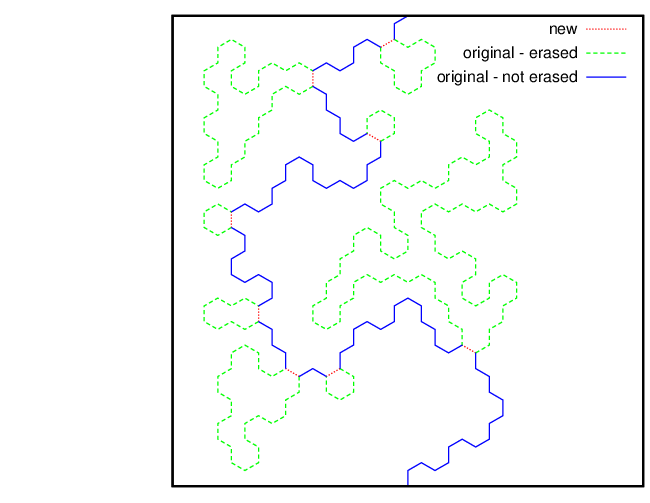

The percolation explorer starting at and ending at generates the same path as the percolation explorer starting at and ending at . However, it is easy to see from considering examples that the loop-erased percolation explorer depends on the direction in which we traverse the path. We will always use to label the starting point and to label the terminal point. For the LERW simple examples show that we can get a different path when we loop-erase the random walk in reverse chronological order. Nonetheless, the distribution of the LERW using reverse chronological order is the same as the distribution of the original LERW [7]. This property is known as reversibility. Our simulations indicate that the loop-erased percolation explorer is reversible in the scaling limit. We have not investigated if the discrete model is reversible before we take the scaling limit.
When we erase the near-loops in the percolation explorer we obtain a new curve which is smoother than the original percolation explorer in the sense that it has smaller fractal dimension. (The SLE6 trace has fractal dimension [2].) The relation of the loop-erased percolation explorer to the original percolation explorer is similar to the relation of the perimeter of a percolation cluster to the external or accessible perimeter of the cluster defined as follows. The cluster will have deep fjords which are connected to the complement of the cluster only through an opening whose width is on the order of a lattice spacing. If we fill in these deep fjords, the perimeter of the resulting object is called the external perimeter of the cluster. It can also be defined by considering adsorbent particles with a diameter that is slightly larger than the lattice spacing [4, 5, 1]. If we follow the perimeter of a percolation cluster, the near-loops will be of two types - those forming a deep fjord into the cluster and those forming a blob that is just barely attached to the cluster. If we only erase the near-loops forming fjords, we will obtain the external perimeter of the cluster.
2 Tests of conformal invariance
We test the conformal invariance of the loop-erased percolation explorer by simulating it for four different domains (square, equilateral triangle, half-disc and disc) which we will denote by S,T,H,and D. We also use several choices of the starting point and terminal point . They are shown in figure 3. For the square we have two choices of starting and terminal points. They are labeled a and b in the figure. For the triangle T we have four choices of starting and terminal points. Choices a,c and d are shown in the figure. Choice b is given by reversing the direction of choice a. For the half-disc H, choices a and c are shown in the figure. Choice b is the reversal of a. Finally, for the disc D there is only one choice of starting and terminal points. So there are ten choices of region and starting/terminal points which we label Sa, Sb, Ta, Tb, Tc, Td, Ha, Hb, Hc, Da.
We can take the scaling limit by fixing the domain and introducing a lattice with spacing which is then sent to zero, or by taking the lattice spacing to be and letting the scale of the domain go to infinity. We do the latter. The length is indicated for each domain in the figure. For the triangle, half-disc and disc we have done simulations with . These values are chosen so that is increasing by approximately a factor of . The domain in the simulation is made up of hexagons, so it is only an approximation to the true domain. As varies the approximating domain can change in a somewhat irregular way. As a result the finite effects can show a somewhat chaotic dependence on . As we will see in detail later, this chaotic dependence is not that significant for the triangle, half-disc and disc. However, it can be quite pronounced for the square. The reason is that the approximating domain is a rectangle of hexagons, but the aspect ratio of this rectangle is not . As varies this aspect ratio changes enough to produce noticeable chaotic dependence of the finite effect on . We have found that this can be greatly reduced by choosing values of for which the aspect ratio does not vary so much. The values do this, so these are the values we use for the simulations for the square.

We test conformal invariance in two ways. The first uses a family of random variables. Fix a conformal map from the domain to the upper half plane which sends the starting point to the origin and the terminal point to . (There is a one parameter family of such maps.) We let be the curve in the domain whose image under is a semicircle of radius centered at the origin. We find the first point where the loop-erased percolation explorer crosses the curve . The random variable is the polar angle of . (For convenience we divide this angle by .) Just how this random variable depends on depends on the choice of , so we do not parameterize the random variable by but rather by a parameter defined as follows. Consider the intersection of with the line from the starting point to the terminal point. Then is the distance from the starting point to this intersection divided by the distance from the starting point to the terminal point. If the scaling limit is conformally invariant, then the distribution of this random variable will be the same for all domains, all choices of and all choices of the parameter . We will refer to this random variable as the “first hit” random variable.
The second test of conformal invariance uses the probability of passing right of a point in the domain. If we take a conformal map from our domain to the upper half plane which sends to and to , then this probability only depends on the polar angle of . Rather than compute this probability for a single point, we compute it for a sequence of points along a line segment in the domain. We parameterize the line segment by , and look at the probability of passing right of the points on the line as a function of . We will refer to this function as the “pass right function.” If the model is conformally invariant then the pass right function will be the same for all domains, all choices of and all choices of the line in the domain. Note that the image of the line under the conformal map is usually not a semi-circle in the half-plane, but this does not matter since the probability of passing right of a point in the upper half plane only depends on the polar angle, not on the radius. The line segments we use for our different choices of domains and starting points are all horizontal or vertical. For Sa, Sb, Ta, Tb, Ha, Hb, and Da, the line segment is horizontal. For Tc, Td and Hc it is vertical. The position of the line segment is parameterized by . The position is linear in with corresponding to the line segment passing through the point where the explorer starts and to the line segment passing through the termination point.
Before we take the scaling limit, the random variable we are studying is discrete since there are only a finite number of points where the loop-erased percolation explorer can first hit the curve . So the cumulative distribution function (cdf) is a step function. Similarly, the pass right function is a step function before the scaling limit. In the scaling limit these step functions should converge to smooth functions, but for the lattice spacings that can be simulated the effect of this discreteness is quite noticable. We can reduce the effect of this discreteness in the following way. Rather than consider the first hit random variable for a single value of , we average the random variable over some interval for . If the loop-erased percolation explorer is conformally invariant, then the cdf of this averaged random variable will be independent of the interval we average over, as well as the domain and starting and terminal points. As varies the finite set of where the cdf jumps changes, so this averaging over reduces the effect of the discreteness of the random variable for a fixed . Similarly we can reduce the effect of the discreteness for the pass right function by averaging over an interval. For both the first hit random variable and the pass right function we average over three intervals: , and .


In our simulations to test the conformal invariance we generated samples for each of the thirty cases (10 possibilities for the region and starting/terminal points and 3 possibilities for the interval over which we average ). When we compute a cdf or the pass right function we are computing a probability for each value of . Since our samples are independent, the variance for our estimate is . So for around , two standard deviations is approximately . We have not included these error bars in our plots of the first hit random variable cdf or the pass right function to keep the figures from being too cluttered, except in figure 8.
Figure 4 shows the cdf of the first hit random variable for Sa, Ta, Ha and Da and for all three different intervals for . There are curves in the figure, but they look identical in the main plot. The inset blows up a tiny portion of the main plot to illustrate the size of the differences in the curves. In the inset the differences are roughly , and this is typical for all . Figure 5 shows the pass right function for the same four cases of regions and starting/terminal points and all three choices of intervals for . Again, the curves in the main plot are indistinguishable. The differences for these 12 curves are also roughly . The dashed curve in the figure is the exact result for the pass right function for SLE8/3.
To “zoom in” on these plots we will subtract off a reference function. We do not have conjectures for what this first hit cdf and the pass right function are, so for our reference functions we just average four of the cases. We use Sa, Ta, Ha, Da with the parameter averaged over . Figure 6 shows the cdf minus the reference function for the ten choices of region and starting/terminal points. We only show the curves for the simulations with the parameter averaged over . Figure 7 shows the pass right functions for the same ten cases minus the pass right reference function.
The results in figures 6 and 7 only use a single value of and there is no attempt to extrapolate to . Figure 8 shows the difference between the cdf for and the reference function for Ta. Even with the averaging of the parameter , the cdf’s and pass right functions are not smooth enough to extrapolate these functions point wise. We will instead study their Fourier coefficients for several values of and attempt to extrapolate them to .


Our functions are defined on and we compute the Fourier coefficients in the expansion
| (4) |
For the RV we compute the Fourier coefficients of the density rather than the cdf. Since the density has the symmetry , the are all zero. And since it has integral , . So we only compute . The pass right function satisfies . This implies and all the rest of the are zero. So we only compute .
As changes, the way in which our domains are approximated with hexagons changes in a somewhat erratic way. So even the Fourier coefficients have a somewhat chaotic dependence on . In figure 9 we plot the Fourier coefficient for the cdf as a function of for regions Ta, Ha, Da, Sa with the parameter averaged over . The lines are least squares fits to the data. We will use the intercept with the vertical axis as the extrapolation of the coefficient to . Figure 10 shows the analogous plots for the Fourier coefficient for the pass right function.


Our next two plots show the extrapolated Fourier coefficients for all ten choices of domain and and all three choices of the interval for averaging for the first hit random variable density (figure 11) and the pass right function (figure 12). Going from left to right, the order of the domains is Ta, Tb, Tc, Td, Ha, Hb, Hc, Da, Sa, Sb with three data points for each domain corresponding to averaging the parameter over the usual three intervals - , and . We plot the extrapolated values for the five largest Fourier coefficients for these thirty cases. If the model is conformally invariant then all thirty cases should give the same values for the Fourier coefficients. As the plots show, the values for the Fourier coefficients are very nearly the same. The error bars shown in the plots are the statistical errors from the Monte Carlo simulation. There is also error arising from the extrapolation to . This is difficult to estimate given the somewhat chaotic dependence of the Fourier coefficients on .


3 Dimension of the curve

The average distance the loop-erased percolation explorer travels as a function of the number of steps should be asymptotically proportional to for some exponent . The fractal dimension of the curve is . In our simulations the distance between the starting and terminal points of the loop-erased percolation explorer is fixed and the number of steps it takes to travel that distance is random. The average number of steps should be asymptotically proportional to . We have computed this average number of steps for the triangular region for values of ranging from to with samples for each value of .
To estimate accurately we must take into account the next order term. Let be the average number of steps. We assume . So
| (5) | |||||
This is linear in the unknown parameters and , but not in . For a given value of we do a weighted least squares fit to find and . We then search over to find the value that minimizes the residual sum of squares (RSS). We find the RSS is minimized when and for this , . We emphasize that the error bars on are only the error from the Monte Carlo. There is also error from the neglected higher order terms in eq. (5). Figure 13 shows a plot of as a function of . The curve shown is . It fits the data quite well, supporting our ansatz (5).
Since the numerical estimate of is very close to , if the loop-erased percolation explorer is some SLEκ, then must be very close to . For SLE, Schramm found an explicit formula for the pass right function [12]. Figure 5 includes Schramm’s result for (the dashed curve). It is clearly different from the pass right function computed in our simulations, leading us to conclude that the loop-erased percolation explorer is not an .
4 Loop-erasing with a gap of
Our definition of the loop-erasure process was that when the percolation explorer comes within one lattice spacing of itself, we erase this near loop and replace it with a single bond. From now on we will refer to this as loop-erasure with a gap of . Now we will consider loop-erasure with a gap of . Loosely speaking we consider the percolation explorer to have formed a loop when it comes within two lattice spacings of itself. We erase such a near loop and replace it with two bonds. (Note that unlike the square lattice, on the hexagonal lattice there is only one choice for the two bonds.)
However, the above definition is a bit too simplistic. Suppose that are times such that , i.e., the loop at time has returned to within lattice spacings of its past. Suppose that the next step after time brings the loop within lattice spacing of , i.e., . Then replacing the near-loop from to with the two bonds from to will result in a path in which the bond from to is traversed twice. So we define loop-erasure with a gap of as follows.
We start by defining . Unlike the definition when the gap is , it is no longer true that all the sites in the loop-erased explorer are sites in the original explorer. For such that is a site in , we define by . Now suppose we have defined , and is such that is a site in . If we stop and set . Note that and are two of the three nearest neighbors of . Let denote the third nearest neighbor of . We first check if there is a such that , i.e., a gap of size . If so, we set and . In this case the definition of the loop-erased explorer is extended by one step. If there is not such a , we check if there is a such that is a nearest neighbor of . If there is, then we set and . We have and is not defined since is not a site in . In this case the definition of the loop-erased explorer is extended by two steps. Finally, if we did not find a gap of size or , then we set and so .
In this section we study whether the loop-erased percolation explorer using a gap of has the same scaling limit as the loop-erased percolation explorer using a gap of . We study this question by computing the same two quantities that we did for the case of a gap of , namely, the first hit random variable and the pass right function. We compute the Fourier coefficients of the density of the random variable and of the pass right function for the same set of lengths as we did for a gap of 1. Then we extrapolate them to just as we did before. We have only done these computations for Sa, Ta, Ha and Da and for all three intervals for averaging . So we have 12 cases instead of 30 as before. In figure 14 we plot the extrapolated values for the five largest Fourier coefficients for the density of the first hit random variable. The 12 cases for erasing using a gap of are on the left. From left to right the domains are Ta, Ha, Da, Sa with three data points for each domain for the three interval for . On the right we show our previous results for erasing using a gap of for the same 12 cases. The analogous plot for the five largest Fourier coefficients for the pass right function is figure 15. As can be seen in these two figures, the results for a gap of 1 and a gap of 2 appear to be the same.


5 Macroscopic difference of loop-erasures
Suppose we take a percolation exploration process curve and loop-erase it in two different ways - one using a gap of and the other a gap of . We let and be the resulting two curves. As before we take the lattice spacing to be and take the scaling limit by letting . So we need to rescale the curves by a factor of to take the scaling limit. Note that for a given , and are random curves on the same probability space. The conclusion of the previous section is that and converge in distribution to the same process. So the distributions of and are close when is large. Since these two curves are defined on the same probability space (which depends on ), we can ask if the two curves are close with high probability. (The convergence in distribution does not imply that they must be close.) More precisely we can ask if for all we have
| (6) |
where is some distance function for curves.
Computing the distance between two curves is computationally intensive since we must consider all possible parameterizations of the curves. So we will study a different quantity to test if and are close. Let be a curve which goes from one boundary point of the domain to another boundary point in such a way that it disconnects the starting and ending points. So the curves and must cross at least once. Let parameterize by arc-length, normalized so that runs from to . For the point corresponding to parameter value , let be if passes right of the point with parameter value , if it passes left. The quantity is then the indicator function of the event that one of and passes right of the point and the other passes left of the point. We will study the following random variable:
| (7) |
So computes the fraction of the curve where one of or is right of the point and the other is left of the point.
Our simulations will show that does not converge to zero. Strictly speaking, not being small does not imply that is not small. It is possible that the two curves stay very close to each other but oscillate back and forth across in such a way that is not small, but this sort of behavior is not expected. We will see in the simulations that for finite , is nonzero but it is decreasing as . The tricky question is whether it converges to zero or not as .
We study just for Ta. We take the curve to be a horizontal line which is a distance above the base of the triangle. (Recall that is the height of the triangle.) The parameter is averaged over . The equilateral triangle T has the advantage that it can be approximated by hexagons in a regular way. We have simulated a large number of values of to study the limit carefully. We use , , , , , , , , , , , , and with samples computed for each value. These lengths were chosen so that the ratio of consecutive lengths is very nearly .
Figure 16 shows the cdf of for and . Since is equal to where is the cdf of , the expected value is equal to the area between the cdf of , the horizontal line with height and the vertical axis. We need to determine if this area goes to as .

If goes to zero, it is natural to expect it goes as for some power . So a log-log plot of as a function of would be linear. The top curve in figure 17 shows this log-log plot. It is not linear but rather is slightly convex. The line shown as a guide to the eye has slope . If goes as , then since our values of are essentially growing geometrically, the differences between values of for successive values of should go to zero as . The lower curve in figure 17 is a log-log plot of the differences. It is noisy but looks to be linear with slope around . Note that this slope is quite different than the slope of the top line in the figure. We have multiplied the data for the bottom curve by a factor of so that the two curves can be shown in a single figure.

If goes as , then it should be a linear function of . So we plot as a function of in figure 18. Note that this is not a log-log plot. The data is very well fit by a linear function with a vertical intercept that is clearly not zero. This plot is the best evidence that does not converge to zero as .

6 Conclusions
The bulk of our Monte Carlo simulations have been for the loop-erased percolation explorer in which we consider the process to have formed a loop when it comes within one lattice spacing of a site it has visited before (the gap=1 model). These simulations give strong support to three conjectures:
Conjecture 1.
The scaling limit of the loop-erased percolation explorer is conformally invariant.
Conjecture 2.
The fractal dimension of the scaling limit of the loop-erased percolation explorer is . (This is the dimension of SLE8/3.)
Conjecture 3.
The scaling limit of the loop-erased percolation explorer is not SLE8/3.
We have also carried out simulations in which the explorer is considered to have formed a loop when it comes within two lattice spacings of a previously visited site (the gap=2 model). These simulations support the conjecture that the gap=1 and gap=2 models converge in distribution to the same limit as the lattice spacing goes to zero. The gap=1 and gap=2 models can be coupled in a trivial way. We take one sample of the percolation explorer and loop-erased that single sample in two different ways to produce one sample, , of the gap=1 model and one sample, , of the gap=2 model. One might expect that if is some distance function on curves, then for all , converges to zero as the lattice spacing goes to zero. However, our simulations provide strong evidence that this is not the case.
Since it appears that the scaling limit of the loop-erased percolation explorer is a conformally invariant process that is not any SLEκ, an obvious question is what is it? A natural conjecture is that it is some SLE() process. If the dimension of the curves is as the simulations indicate, then would have to be . But we see no obvious conjecture for the other parameter(s).
As for future work, one could consider loop-erasing other lattice models whose scaling limit is SLEκ with , e.g., FK percolation, and ask if the scaling limit is conformally invariant. One could also attempt to define a loop-erasure process for SLEκ itself when . The difficulty of course is that there is no natural linear chronological order for the loops.
Acknowledgments: This research was supported in part by NSF grant DMS-1500850. An allocation of computer time from UA Research Computing at the University of Arizona is gratefully acknowledged.
References
- [1] M. Aizenman, B. Duplantier, A. Aharony, Path-crossing exponents and the external perimeter in 2D percolation. Phys. Rev. Let. 83 , 1359–1362, (1999).
- [2] V. Beffara, Hausdorff dimensions for SLE6. Ann. Probab. 32 2606–2629 (2004).
- [3] F. Camia, C. M. Newman, Critical percolation exploration path and SLE6 : a proof of convergence. Probab. Theory Related Fields 139,473–519 (2007).
- [4] T. Grossman and A. Aharony, Structure and perimeters of percolation clusters. J. Phys. A: Math. Gen., 19, L745 (1986).
- [5] T. Grossman and A. Aharony, Accessible external perimeters of percolation clusters. J. Phys. A: Math. Gen., 20, L1193 (1987).
- [6] G. F. Lawler, A self-avoiding walk, Duke Math. J., 47, 655–694 (1980).
- [7] G. Lawler, A connective constant for the loop-erased self-avoiding walk, J. Appl. Prob. 20 264-276 (1983).
- [8] G. Lawler, Conformally Invariant Processes in the Plane. American Mathematical Society (2005).
- [9] G. Lawler, O. Schramm, W. Werner, Conformal Invariance of Planar Loop-Erased Random Walks and Uniform Spanning Trees. Ann. Probab. 32, 939–995, (2004).
- [10] S. Rohde, O. Schramm, Basic properties of SLE. Ann. Math. 161 883–924 (2005).
- [11] O. Schramm, Scaling limits of loop-erased random walks and uniform spanning trees. Isr. J. Math. 118, 221–288 (2000).
- [12] O. Schramm, A percolation formula. Electron. Comm. Probab. 6, 115–120 (2001).
- [13] S. Smirnov, Critical percolation in the plane: Conformal invariance, Cardy’s formula, scaling limits. C. R. Math. Acad. Sci. Paris 333, 239–244 (2001).
- [14] W. Werner, Lectures on two-dimensional critical percolation, Statistical Mechanics (IAS/Park City mathematics series v. 16), S. Sheffield, T. Spencer (eds.) (2007).