Non equivalence of dynamical ensembles and emergent non ergodicity

The Markov jump process $X_{t}$ takes values in the finite state space $\Omega$ at all time $t\in[0,T]$. The probability that $X_{t}=x\in\Omega$ at time $t$, denoted $p(x,t)$, is the solution of the time-homogeneous master equation

where $K(x,y)$ are the components of the Markov operator $\bm{K}$, i.e. the probability per unit time of the transition from $y$ to $x$. The Markov jump process is said to be irreducible if for any pair of states $x\neq y$ it exists a path that connects $x$ to $y$ (and $y$ to $x$), i.e. every transitions along the path have non-vanishing transition rates. On the opposite, the process is reducible when at least two subsets of states in $\Omega$ cannot be connected. Then, the process is non-ergodic. As a consequence, the ensemble average does not produce the same result as the time average since the process cannot explore the whole state space.

Alternatively, one may use the path-integral formalism to characterize the process $X_{t}$. In this case, we denote by $P[x]$ the path probability, where $[x]$ is the short notation for a realization of the process $X_{t}$ over the time interval $[0,T]$.

We aim at computing the statistics of a dynamical observable $\mathcal{O}$. The mean value of this observable $\mathcal{O}$ follows from

where $\int\mathcal{D}[x]$ denotes the sum over all possible paths. For simplicity, we consider an observable of the form

where $f(x)$ and $g(x,y)$ are arbitrary functions and the discrete sum is on the time $t$ at which the system changes of state, i.e. $\Delta X_{t}\equiv X_{t^{+}}-X_{t^{-}}\neq 0$. The $f$ dependent part enables to study the time average of a state function, and the $g$ dependent part the time average of jump quantities, like currents. For example, choosing $f(x)=0$ and $g(x,y)=1$ will lead to the global activity of the system, i.e. the number of jumps per unit time in the trajectory.

The microcanonical ensemble is defined by filtering the trajectory ensemble with a condition on an observable, e.g. $\mathcal{O}=\mathfrak{o}$ where $\mathfrak{o}$ is a possible value of the stochastic variable $\mathcal{O}$ such that its probability verifies $P_{T}(\mathcal{O}=\mathfrak{o})>0$. We write the path probability of these trajectories

where $P^{\mathfrak{o}}[x]$ is the conditional probability of the path $[x]$ given that for this path $\mathcal{O}=\mathfrak{o}$. The corresponding joint probability is denoted $P[x,\mathcal{O}=\mathfrak{o}]$. In the microcanonical path ensemble, the observable $\mathcal{O}$ does not fluctuate and always achieves the same value for all trajectories in the ensemble.

The canonical ensemble is defined by fixing the mean value of the observable $\mathcal{O}$ only. The path probability for this ensemble can be computed via tilting (or biasing) the process as follows:

This path probability is normalized by construction.

To discuss the dynamical ensemble equivalence, one needs to define when two path probabilities $P$ and $Q$ are equivalent. They do when

almost everywhere with respect to $P$. This means that $P$ and $Q$ are equal up to subexponential terms in $T$ for almost all paths. As a consequence, the mean value at large time of any observable will be the same if computed with any one of the two equivalent path ensembles.

Assuming a large deviation principle for $\mathcal{O}$ [10], the LDF function $I(\mathfrak{o})$ provides the rate of decay of the probability density function $P_{T}(\mathcal{O}=\mathfrak{o})$ in the limit $T\to+\infty$ such that

A LDF indicates the rate at which the probability density function of a time extensive observable concentrates in its most likely value when time goes by.

Assuming a large deviation principle, Chetrite and Touchette have shown that the convexity of $I(\mathfrak{o})$ determines whether the microcanonical and canonical path ensembles are equivalent [11], in such a case $P^{\mathfrak{o}}$ and $P_{\gamma}$ satisfy Eq. (6). They distinguished three cases:

• (Equivalence) If $I(\mathfrak{o})$ is a stricly convex function at $\mathfrak{o}$, then there exists a unique $\gamma\in\mathbb{R}$ such that $P^{\mathfrak{o}}$ and $P_{\gamma}$ are equivalent.

• (Non equivalence) If $I(\mathfrak{o})$ is a non-convex function at $\mathfrak{o}$, then there are no $\gamma$ such that $P^{\mathfrak{o}}$ and $P_{\gamma}$ are equivalent.

• (Partial equivalence) If $I(\mathfrak{o})$ is a convex function but not strictly convex function at $\mathfrak{o}$, then numerous values of $\mathfrak{o}$ correspond to the same $\gamma$: It may correspond to linear parts in a convex function or to a point of a non-convex function at which the slope is not unique.

The convexity of the LDF $I(\mathfrak{o})$ is connected to the differentiability of the CGF. The CGF $\phi(\gamma)$ is defined as

The CGF is the highest eigenvalue of the titled matrix $\bm{K}_{\gamma}$ of elements [33]

The CGF is also the Legendre-Fenchel transform of the LDF

Conversely, we define $I^{**}(\mathfrak{o})$ as the Legendre-Fenchel transform of the CGF

with $\gamma(\mathfrak{o})$ the value of $\gamma$ realizing the maximum. The Gärtner-Ellis theorem states that if $\phi(\gamma)$ is a differentiable function then $I(\mathfrak{o})=I^{**}(\mathfrak{o})$. The properties of the Legendre-Fenchel transform implies that $I^{**}(\mathfrak{o})$ is a convex function. The strict convexity of the LDF and the differentiability of the CGF are then dual conditions. Therefore we have the three following cases:

• (Equivalence) If $\phi(\gamma(\mathfrak{o}))$ is differentiable at $\gamma(\mathfrak{o})$, then $I(\mathfrak{o})=I^{**}(\mathfrak{o})$ from the Gärtner-Ellis theorem, and moreover $\mathfrak{o}=\partial_{\gamma}\phi(\gamma)$. $I(\mathfrak{o})$ is then a strictly convex function at $\mathfrak{o}$ and the equivalence holds.

• (Non equivalence) If $\phi(\gamma(\mathfrak{o}))$ is not differentiable at $\gamma(\mathfrak{o})$ and $I(\mathfrak{o})\neq I^{**}(\mathfrak{o})$, then $I(\mathfrak{o})$ is a non-convex function at $\mathfrak{o}$ and we have a non equivalence between the microcanonical and canonical ensembles.

• (Partial Equivalence) If $\phi(\gamma(\mathfrak{o}))$ is not differentiable at $\gamma(\mathfrak{o})$ and $I(\mathfrak{o})=I^{**}(\mathfrak{o})$, then $I(\mathfrak{o})$ is a convex function but not strictly convex function at $\mathfrak{o}$ and we have a partial equivalence between the microcanonical and canonical ensembles.

Hence, the non-equivalence of ensembles prevents to compute the LDF from the CGF since $I^{**}(\mathfrak{o})$ is only the convex hull of $I(\mathfrak{o})$. In Ref. [11], the authors conjectured a connection between non equivalences and non ergodicity. We support this idea in the following by confirming that non-ergodicity is required to observe a non equivalence of ensemble, but it is not a sufficient condition.

The proof of ensemble equivalence amounts to determine the convexity of a LDF function. In this section, we show how the LDF for observable $\mathcal{O}$ can be determined from the convex LDF of more general observables, and how the convexity property may be inherited in the process.

Whenever a stochastic variable depends of a set of other stochastic variables, one can infer the LDF of the former from the LDF of the latters. This operation is called a contraction. For instance, the observable $\mathcal{O}$ of Eq. (48) is a function of the empirical occupation ratio $R$ and the jump rate $C$

The occupation ratio is defined as the relative time spent in each state, say $x$ here

where $\delta$ is an indicator function being $1$ if the condition is satisfied and $0$ otherwise. The jump rate $C(x,y)$ counts the number of transitions between two states (from $y$ to $x$) per unit time

The occupation ratios and the jump rates have a joint probability for $R=r$ and $C=c$ that satisfies a large deviation principle

defining the large deviation function $I(r,c)$, also called the level 2.5 LDF[34, 35, 36]. Then, the contraction

leads to the LDF for the observable $\mathcal{O}$. In general terms, a contraction corresponds to the minimization of a multivariate LDF under a condition encoding how the stochastic variables are related [10].

Since ensemble equivalence for a stochastic variable relies on the convexity of the corresponding LDF, it is crucial to determine (i) whether the LDF $I(r,c)$ is convex and (ii) whether the convexity can be inherited upon contraction. The following theorem appearing in Ref. [37] provides an answer to point (ii) when the new variable is additive:

We now address the point (i) about the convexity of the LDF $I(\bm{r},\bm{c})$. This level 2.5 LDF is explicitly known for ergodic Markov jump processes in continuous-time [34, 35, 36]

It is convex since it writes as the sum of a linear part $\sum_{x,y\neq x}\left[r(y)K(x,y)-c(x,y)\right]$ and a Kullback-Leibler divergence between $\bm{c}$ and $\bm{Kr}$

This Kullback-Leibler divergence is convex as a consequence of the log-sum inequality (or Jensen’s inequality) [38]. Using the previous theorem with $\bm{z}=(\bm{r},\bm{c})$, the convexity of the level 2.5 LDF and the additivity of $\mathcal{O}$ for both the occupation ratio and the jump rate, we conclude the contracted LDF $I(\mathfrak{o})$ is also convex: The ensemble equivalence holds for ergodic Markov jump processes. In particular, the ensemble equivalence holds for irreducible finite size Markov jump processes since they are always ergodic.

Alternatively, one can prove heuristically the ensemble equivalence using the differentiability of the CGF, that is the dual condition with respect to the LDF convexity. To determine the CGF differentiability, one consider the CGF as the highest eigenvalues of the titled matrix $\bm{K}_{\gamma}$ defined in Eq.(65). From Perron-Fröbenius theorem for irreducible finite size matrices like $\bm{K}_{\gamma}$, the highest (real) eigenvalue is unique: Its multiplicity is always one independently of the value of the counting field and no crossing between the two highest eigenvalues can occur. Moreover, the components of the tilted matrix are differentiable yielding that the CGF is itself differentiable. By duality, the LDF is strictly convex.

From this analysis, we conclude that the non-equivalence between the microcanonical and canonical ensembles based on observables like $\mathcal{O}$ may only happen when the Markov operator is reducible or of infinite dimension. Then, the LDF of the variable $\mathcal{O}$ may not be convex.

We emphasize that we made no assumption on the definition of dynamical rates, hence the system may be in or out of equilibrium. We used simple graph Markov processes, but the discussion can be transposed to include multiple channel transitions.

Let’s consider a four state system made of two subsystems with two states $(1,2)$ and $(3,4)$. The four state system evolves according to the master equation

The Markov operator is reducible yielding to a non ergodic process. We aim at computing the system activity assuming that one cannot distinguish in which subsystem a transition occurs. The activity rate $A$ is the total number of jumps per unit time: It is given by Eq. (48) when $f(x)=0$ and $g(x,y)=1$ for all $(x,y)$. By definition of the Markov operator in the right hand side of Eq. (21), the activity probability distribution of each subsystem is a Poisson distribution of mean value $T$ for the subsystem $(1,2)$ and $2T$ for the subsytem $(3,4)$, because there is $1$ and $2$ jumps per unit time in each subsystem respectively. The probability distribution of the total number of jumps is the sum of Poisson distributions weighted by the initial probability $p_{\mathrm{i},n}$ to start in state $n$. The probability of having $aT$ jumps after a time $T$ is

For $T$ large enough, $P_{T}(A=a)$ will be bimodal, and the microcanonical LDF reads

where we have used Stirling formula and chosen the minimum of the two LDF corresponding to each Poisson distribution. The above microcanonical LDF of activity is shown in Fig. 1b. It is crucial to note that the initial condition plays a fundamental role here: if the system never starts in states $1$ or $2$, i.e. $p_{\mathrm{i},1}=p_{\mathrm{i},2}=0$, the LDF will include the branch corresponding to the second line of Eq. (23) only. The non-ergodicity impacts the long time statistics of the dynamical observables through the choice of initial conditions.

For the four state model, it is straightforward to determine the probability density function of activity, but for other systems or observables this task may be more challenging: one must often compute the CGF instead. Let’s derive the result of Eq. (23) in this way using the propagator for the generating function of the activity defined by $G(x_{\mathrm{f}},x_{\mathrm{i}},\gamma)=\langle e^{T\gamma A}\rangle_{x_{\mathrm{f}},x_{\mathrm{i}}}$, where the subscripts $x_{\mathrm{i}}$ and $x_{\mathrm{f}}$ denote respectively the initial and final states of the trajectories appearing in the average. Using standard approach [39, 10], the propagator is obtained from the biased operator

as the components of its matrix exponential $\left[\exp(T\bm{K}_{\gamma})\right](x_{\mathrm{f}},x_{\mathrm{i}})=G(x_{\mathrm{f}},x_{\mathrm{i}},\gamma)$. Using eigenvalues and eigenvectors decomposition of $\bm{K}_{\gamma}$, we make explicit the matrix exponential

The orthogonal basis of eigenvectors has normalized right eigenvectors, and the scalar products of the left and right eigenvectors associated to the same eigenvalue are all equal to $1$. We notice that the eigenvectors separate in two sets whose supports are disjoints and correspond to each subsystem respectively. We remark also that the above propagator should be norm conserving when $\gamma=0$, but the two terms in the second line of Eq. (25) do not fulfill this requirement. We do not consider then as physical and keep only the two first terms in Eq. (25). Then, the activity LDF is recovered from this propagator by first summing over the initial and final states

second, applying an inverse Laplace transform, and finally by taking the limit $T\rightarrow\infty$. For ergodic systems, this procedure leads to the same LDF whatever the order of these operations. On the contrary, the order matters for non-ergodic systems.

For our $4$ state model, the generating function writes

Its inverse Laplace transform yields the probability density function of activity given in Eq. (22). However, first computing the long time limit of the generating function leads to the CGF

as long as $p_{\mathrm{i}}(x)>0$ for all x. Noticing that the limit $T\to+\infty$ enables to use a saddle-point method to approximate the inverse Laplace transform into a Legendre-Fenchel transform, the asymptotic probability of activity follows from its corresponding LDF

that is not the one of Eq. (23). The above LDF is convex because a Legendre-Fenchel transform only yields convex functions by definition, while the LDF of Eq. (23) is not convex.

Alternatively, one may obtain the microcanonical LDF by taking the long time limit on the propagator of the generating function of Eq. (25), and not on the generating function itself, yielding

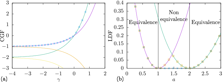
The Legendre-Fenchel conjugate of these two branches associated to different initial states are precisely the two branches of the microcanonical LDF in Eq. (23):

The summation over initial and final conditions is now carried out using an asymptotic approximation, which can be written heuristically as

explaining why a minimum on the branches of Eq. (31) appears in the final microcanonical LDF of Eq. (23). To summarize, from the Legendre-Fenchel conjugate of all the eigenvalues appearing in the biased operator of Eq. (24), we determined the partial LDFs. The minimum among these partial LDFs produces the microcanonical LDF. We illustrate this procedure in Fig. 1. From this figure, we conclude on the ensemble equivalence for this model: it holds for $a\in[0,1[\,\bigcup\,]2,+\infty[$, but the equivalence is partial at $a={1,2}$ and there is no equivalence for $a\in]1,2[$.

Remark that when the mean activities of each subsystem are the same, the two branches of the LDF merge toward a convex shape. Therefore, in this case non-ergodicity is not sufficient to observe ensemble non-equivalence associated to non-convexity of the LDF.

In the above example, we have seen that one can determine the asymptotic fluctuations of a physical observable by switching from one dynamical ensemble to another as long as the LDFs are piecewise-convex. In this section, we develop this approach for the more general framework of section II. In practice, this amounts to express the inverse Laplace transform as a Legendre-Fenchel transform, using the saddle point method and taking care of the initial condition appropriately.

By definition, for $b\in\mathbb{R}$, the microcanonical LDF for $\mathcal{O}$ writes

in term of the initial probability $p_{\mathrm{i}}(x_{\mathrm{i}})$ and of the propagator $G(x_{\mathrm{f}},x_{\mathrm{i}},\gamma)=\langle e^{T\gamma\mathcal{O}}\rangle_{x_{\mathrm{f}},x_{\mathrm{i}}}$ that generates the moments of $\mathcal{O}$ under given initial and final conditions. The argument of the logarithm in Eq. (33) is exactly the probability distribution function of $\mathcal{O}$. Since solely the most probable events contribute to the LDF, we can focus on the initial conditions leading to the minimal value of the LDF (as seen in section III.1):

Finally, the complex integral for the inverse Laplace conjugate follows from the saddle point method:

Alternatively, the convex hull of $I_{\textrm{mc}}(\mathfrak{o})$ is the Legendre-Fenchel conjugate of the CGF for the observable $\mathcal{O}$, namely

As seen in section III.1, the propagator $G$ may have an eigendecomposition for which the terms contributing to the CGF in the limit $T\to\infty$ depend on the initial or final condition. Hence, a maximum on $x_{\mathrm{f}}$ and $x_{\mathrm{i}}$ must appear

to select the dominant asymptotic behavior in the limit $T\to\infty$. In view of comparing with Eq. (35), the maximization is modified into a minimization through the commutation with the minus sign:

In the end, the difference between the LDF $I_{\textrm{mc}}(\mathfrak{o})$ and its convex hull $I_{\textrm{c}}(\mathfrak{o})$ comes from the non commutation of $\max_{\gamma}$ and $\min_{x_{\mathrm{f}},x_{\mathrm{i}}}$ as a consequence of the dependence on the initial conditions, i.e. of the non-ergodicity. Of course, if the LDF were convex, the ordering of these extremization would not matter.

The eigendecomposition of the propagator $G$ involves the eigenvalues of the biased matrix of Eq. (65). For non-ergodic systems or when the state space is infinite, the assumption of the Perron-Frobenius theorem does not hold and several eigenvalues may cross each other. To compute exactly the microcanonical LDF, one needs all the branches corresponding to each eigenvalue that becomes the highest eigenvalue for at least one $\gamma$. Only those branches matters, and other eigenvalues will not contribute, so as can be understood from the following argument: Be two eigenvalues $\phi_{1}(\gamma)$ and $\phi_{2}(\gamma)$ such that $\phi_{1}(\gamma)>\phi_{2}(\gamma)$ for all $\gamma$. Since $\gamma\mathfrak{o}-\phi_{1}(\gamma)<\gamma\mathfrak{o}-\phi_{2}(\gamma)$, we have

The last minimization in Eq. (35) on the partial LDFs will withdraw the contribution coming from the eigenvalue $\phi_{2}(\gamma)$ if it is smaller that $\phi_{1}(\gamma)$.

Physically speaking, we study a rare event in a system that has several independent subparts. We assume that the initial probability cannot be zero in all states of a subsytem, otherwise this subsystem shall be ignored. Each subpart of the system has its own probability to realize the rare event at stake. The subpart for which the event is the most likely will determine the event probability. This will be so if the rare event corresponds to a fluctuation of a time average quantity on a sufficiently long time so as to neglect the role of the initial state probability.

Mathematically speaking, when dealing with reducible biased operators whose highest eigenvalue is the CGF of interest, we must divide the operator into irreducible sub-operators for which holds the ensemble equivalence. For every sub-operators we proceed normally using the ensemble equivalence to determine the partial LDFs of the chosen observable from the Legendre-Fenchel transform of the highest eigenvalue of the sub-operator. The final LDF for the total system is then given by the minimum over all partial LDFs. This explains why the final LDF is piecewise convex.

Using the results of sec. III.2, we study the activity and magnetization of an infinite range Ising model. This model is ergodic when considering a finite number of spins, but breaks ergodicity in the thermodynamics limit. In the following, we first introduce the model and its mean field (MF) treatment. Second, we provide the propagator of the generating function for magnetization and activity, and next use it to determine the CGF and both the canonical and microcanonical LDFs.

References

- [1] H. B. Callen, Thermodynamics and an Introduction to Thermostatistics (Wiley, 1985).
- [2] Julien Barré, David Mukamel, and Stefano Ruffo, “Inequivalence of ensembles in a system with long-range interactions,” Phys. Rev. Lett. 87, 030601 (2001).
- [3] Alessandro Campa, Thierry Dauxois, and Stefano Ruffo, “Statistical mechanics and dynamics of solvable models with long-range interactions,” Physics Reports 480, 57–159 (2009).
- [4] Freddy Bouchet, Shamik Gupta, and David Mukamel, “Thermodynamics and dynamics of systems with long-range interactions,” Physica A: Statistical Mechanics and its Applications 389, 4389–4405 (2010), proceedings of the 12th International Summer School on Fundamental Problems in Statistical Physics.
- [5] Richard S. Ellis, Hugo Touchette, and Bruce Turkington, “Thermodynamic versus statistical nonequivalence of ensembles for the mean-field blume–emery–griffiths model,” Physica A: Statistical Mechanics and its Applications 335, 518–538 (2004).
- [6] Marius Costeniuc, Richard S. Ellis, and Hugo Touchette, “Complete analysis of phase transitions and ensemble equivalence for the curie-weiss-potts model,” J. Math. Phys. 46,, 063301,2005. (2005), cond-mat/0410744 .
- [7] Hugo Touchette, Richard S. Ellis, and Bruce Turkington, “An introduction to the thermodynamic and macrostate levels of nonequivalent ensembles,” Physica A: Statistical Mechanics and its Applications 340, 138–146 (2004), news and Expectations in Thermostatistics.
- [8] Freddy Bouchet, Thierry Dauxois, David Mukamel, and Stefano Ruffo, “Phase space gaps and ergodicity breaking in systems with long-range interactions,” Phys. Rev. E 77, 011125 (2008).
- [9] H. Touchette, Equivalence and nonequivalence of the microcanonical and canonical ensembles : a large deviations study, Ph.D. thesis, PhD Thesis Department of Physics, McGill University (2003).
- [10] Hugo Touchette, “The large deviation approach to statistical mechanics,” Physics Reports 478, 1–69 (2009).
- [11] Raphaël Chetrite and Hugo Touchette, “Nonequilibrium markov processes conditioned on large deviations,” Annales Henri Poincaré 16, 2005–2057 (2015).
- [12] Raphaël Chetrite and Hugo Touchette, “Nonequilibrium microcanonical and canonical ensembles and their equivalence,” Phys. Rev. Lett. 111, 120601 (2013).
- [13] Robert L. Jack and Peter Sollich, “Large deviations and ensembles of trajectories in stochastic models,” Progress of Theoretical Physics Supplement 184, 304–317 (2010), http://ptps.oxfordjournals.org/content/184/304.full.pdf+html .
- [14] V. Lecomte, C. Appert-Rolland, and F. van Wijland, “Thermodynamic formalism for systems with markov dynamics,” Journal of Statistical Physics 127, 51–106 (2007).
- [15] Thomas Speck, “Thermodynamic formalism and linear response theory for nonequilibrium steady states,” Phys. Rev. E 94, 022131 (2016), 1601.03540 .
- [16] Juan P Garrahan, “Classical stochastic dynamics and continuous matrix product states: gauge transformations, conditioned and driven processes, and equivalence of trajectory ensembles,” Journal of Statistical Mechanics: Theory and Experiment 2016, 073208 (2016).
- [17] Cécile Monthus, “Non-equilibrium steady states: maximization of the shannon entropy associated with the distribution of dynamical trajectories in the presence of constraints,” J. Stat. Mech. 2011, P03008 (2011).
- [18] Adrián A Budini, Robert M Turner, and Juan P Garrahan, “Fluctuating observation time ensembles in the thermodynamics of trajectories,” Journal of Statistical Mechanics: Theory and Experiment 2014, P03012 (2014).
- [19] Juan P Garrahan, Robert L Jack, Vivien Lecomte, Estelle Pitard, Kristina van Duijvendijk, and Frédéric van Wijland, “First-order dynamical phase transition in models of glasses: an approach based on ensembles of histories,” Journal of Physics A: Mathematical and Theoretical 42, 075007 (2009).
- [20] Willliam Feller, An introduction to probability theory and its applications, Vol. 2 (John Wiley & Sons, 2008).
- [21] Aaron S. Keys, David Chandler, and Juan P. Garrahan, “Using the ensemble to probe glasses formed by cooling and aging,” Phys. Rev. E 92, 022304 (2015).
- [22] Giulio Biroli and Juan P. Garrahan, “Perspective: The glass transition,” The Journal of Chemical Physics 138, 12A301 (2013), https://doi.org/10.1063/1.4795539 .
- [23] Mauro Merolle, Juan P. Garrahan, and David Chandler, “Space-time thermodynamics of the glass transition,” Proceedings of the National Academy of Sciences 102, 10837–10840 (2005), http://www.pnas.org/content/102/31/10837.full.pdf .
- [24] Robert L. Jack, Juan P. Garrahan, and David Chandler, “Space-time thermodynamics and subsystem observables in a kinetically constrained model of glassy materials,” The Journal of Chemical Physics 125, 184509 (2006), https://doi.org/10.1063/1.2374885 .
- [25] J. P. Garrahan, R. L. Jack, V. Lecomte, E. Pitard, K. van Duijvendijk, and F. van Wijland, “Dynamical first-order phase transition in kinetically constrained models of glasses,” Phys. Rev. Lett. 98, 195702 (2007).
- [26] Lester O. Hedges, Robert L. Jack, Juan P. Garrahan, and David Chandler, “Dynamic order-disorder in atomistic models of structural glass formers,” Science 323, 1309–1313 (2009), http://science.sciencemag.org/content/323/5919/1309.full.pdf .
- [27] David Chandler and Juan P. Garrahan, “Dynamics on the way to forming glass: Bubbles in space-time,” Annual Review of Physical Chemistry 61, 191–217 (2010), pMID: 20055676, https://doi.org/10.1146/annurev.physchem.040808.090405 .
- [28] T. Speck and J. P. Garrahan, “Space-time phase transitions in driven kinetically constrained lattice models,” The European Physical Journal B 79, 1–6 (2011).
- [29] Takahiro Nemoto and Shin-ichi Sasa, “Computation of large deviation statistics via iterative measurement-and-feedback procedure,” Phys. Rev. Lett. 112, 090602 (2014).
- [30] Grégoire Ferré and Hugo Touchette, “Adaptive sampling of large deviations,” 1803.11117v1 .
- [31] Hugo Touchette, “Methods for calculating nonconcave entropies,” J. Stat. Mech. P 05008 (2010), 1003.0382 .
- [32] Hugo Touchette, “Simple spin models with non-concave entropies,” Am. J. Phys. 76,, 26–30,2008 (2008), cond-mat/0504020 .
- [33] Joel L. Lebowitz and Herbert Spohn, “A gallavotti–cohen-type symmetry in the large deviation functional for stochastic dynamics,” Journal of Statistical Physics 95, 333–365 (1999).
- [34] C. Maes and K. Netočný, “Canonical structure of dynamical fluctuations in mesoscopic nonequilibrium steady states,” EPL (Europhysics Letters) 82, 30003 (2008).
- [35] Andre C. Barato and Raphael Chetrite, “A formal view on level 2.5 large deviations and fluctuation relations,” Journal of Statistical Physics 160, 1154–1172 (2015).
- [36] L Bertini, Alessandra Faggionato, and Davide Gabrielli, “From level 2.5 to level 2 large deviations for continuous time markov chains,” Markov Processes and Related Fields 20 (2012).
- [37] Stephen Boyd and Lieven Vandenberghe, Convex Optimization (Cambridge University Press, 2004).
- [38] I. Csiszár and P. C. Shields, Information Theory and Statistics: A Tutorial (Now Foundations and Trends, 2004).
- [39] N.G. Van Kampen, Stochastic Processes in Physics and Chemistry (Third Edition), third edition ed. (Elsevier, Amsterdam, 2007).
- [40] Elizabeth L. Wilmer David A. Levin, Yuval Peres, Markov Chains and Mixing Times (American Mathematical Society, 2008).
- [41] Gregory F. Lawler and Alan D. Sokal, “Bounds on the spectrum for markov chains and markov processes: A generalization of cheeger’s inequality,” Transactions of the American Mathematical Society 309, 557–580 (1988).
- [42] Mark I. Freidlin and Alexander D. Wentzell, Random Perturbations of Dynamical Systems, Grundlehren der mathematischen Wissenschaften (Springer-Verlag, New-York, 1984).
- [43] L. Onsager and S. Machlup, “Fluctuations and irreversible processes,” Phys. Rev. 91, 1505–1512 (1953).
- [44] Tobias Grafke, Rainer Grauer, and Tobias Schäfer, “The instanton method and its numerical implementation in fluid mechanics,” Journal of Physics A: Mathematical and Theoretical 48, 333001 (2015).
- [45] Daniel Nickelsen and Hugo Touchette, “Anomalous scaling of dynamical large deviations,” 1803.05708v1 .
- [46] J Szavits-Nossan and M R Evans, “Inequivalence of nonequilibrium path ensembles: the example of stochastic bridges,” Journal of Statistical Mechanics: Theory and Experiment 2015, P12008 (2015).
- [47] Takahiro Nemoto, “Zon-cohen singularity and negative inverse temperature in a trapped-particle limit,” Phys. Rev. E 85, 061124 (2012).
- [48] Roger A. Horn and Charles R. Johnson, Matrix Analysis, 2nd ed. (Cambridge University Press, 2012).
Appendix A Derivation of the propagator for generating function
We look for an expression of the propagator of the generating function as a path integral over all trajectories for the system state . We use the discrete time corresponding to the ’s time step of duration , with the final time . We write the system state for short. This state at time changes by or when a spin jumps from up to down, does’nt jump or jumps from down to up. The sum over all paths for a given initial condition is