Understanding Fashionability: What drives sales of a style?
Abstract.
We use customer demand data for fashion articles on Myntra, and derive a fashionability or style quotient, which represents customer demand for the stylistic content of a fashion article, decoupled with its commercials (price, offers, etc.). We demonstrate learning for assortment planning in fashion that would aim to keep a healthy mix of breadth and depth across various styles, and we show the relationship between a customer’s perception of a style vs a merchandiser’s catalogue of styles. We also backtest our method to calculate prediction errors in our style quotient and customer demand, and discuss various implications and findings.
Keywords:
E-commerce, Style Quotient, Fashionability, Top Sellers, Retail Planning, Inventory Management1. Introduction
A fashion merchandiser builds their inventory by taking several attributes into consideration, such as which fashion article types to carry (eg. women’s tops, kidswear, jeans for all, etc), what they should stand for (premium vs bargain vs fast fashion), and thereby what are the associated design attributes (fabric type, print, details, etc). On the other hand, a customer has a certain emotional connect with fashion that determines what s/he wears, how they shop for fashion, and how they perceive a brand or a retailer. How does a fashion retailer successfully interpret her merchandise in the customer’s view? The answer to this question is the key to building a more relevant inventory, fulfilling changing customer demand, and cutting losses on the long tail of inventory.
At Myntra, every month, about 30 million customers browse, search for, and purchase our collection of about articles that span a range of known big label brands, Myntra’s in-house fashion brands, and a marketplace where several small and medium scale brands list on our platform. Hence, we collect rich data on customer demand as well as available fashion inventory. In this paper, we propose a "Style Quotient" or the customer demand for a fashion product’s (hereby referred as style) content, that is independent of its commercials (price, discount applied, promotional offers, advertising and marketing spend, etc). In order to mirror demand closely out with a full demand picture that is dependent on commercials, and deriving a decoupled style quotient that we propose to use for assortment planning.
2. Style Quotient
When looking at demand data, the choice made by a customer is hard to interpret as solely a matter of preference for the content of the purchased article, as sales are driven by merchandising factors like discount, list views (shelf space allocated in online store), marketing, and promotions. In this work, we show how we infer the influence of stylistic content (such as brand, color, fabric, fit, length, prints) on customer purchases. Today, in the fashion industry Rate of Sales, ROS (Sales Quantity/days live) is used as a proxy for customer preference for stylistic content and we argue that in a highly dynamic environment such as ecommerce, where flash sales, festival discounts, and marketing notifications drive up demand, such a metric is non-representative of “true” customer preferences.
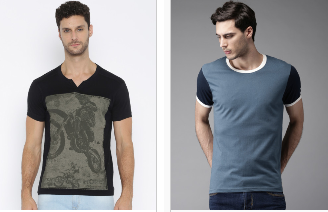
Figure 1 shows two fashion articles (styles) – both with high ROS. Even though both styles have a similar ROS, style (b) is better than style (a) as its demand is less price and promotions driven.
In order to compute the Style Quotient of a particular style listed on Myntra, we pick a subcategory of styles (article type - gender - elementary attributes based) within which comparisons are natural and easy to illustrate. A cross category style quotient can be computed by normalizing for width and depth appropriately, and without loss of generality, we will now deal with a subcategory alone in this paper.
2.1. Data
We consider weekly sales / demand data for our computations. Intuitively, this may circumvent over-fitting due to frequent fluctuations in daily data, and under-fitting due to dissolution and averaging of driving factors in data at a coarser scale. The following attributes of a style are considered in modeling demand driven style quotient. A few attributes are considered in their raw form and others are derived.
- •
Raw:
- –
Sales Quantity: A numerical measure indicating the actual sales of the style.
- –
Is Live: A binary measure indicating whether the style is live on platform or not.
- –
First Time on Discount: A binary measure indicating if the style is put on discount for the first time. This may attract additional traction and increase sales.
- –
Number of styles live from same brand: A numerical measure quantifying the competing styles from the same brand. Many similar styles may lower sales of a particular style.
- –
- •
Derived:
- –
Discount Deviation: Dispersion around average selling price.
- –
Normalised list price:to indicate whether a style is premium or for the mass market.
- –
List Views Deviation: List view is the shelf space allocated to a style in an online store. List views deviation is a numerical measure of style visibility dispersion indicating if a style is attracting higher views as compared to an average for reasons like promotion; making the style noticeable early than others.
- –
Style Age: A measure indicating the shelf life of a style. With longer shelf life, the style’s demand may decay with time.
- –
2.2. Design
We capture the customer preferences for an assortment using ‘demand prediction’ framework. Let there be a universal set = {, , , } which represents the store’s all styles for a given subcategory present in observed time duration . The store’s assortment at week is represented by = { : live at }.
Customers’ preferences is captured as probability of choosing a style at week and is denoted by . Customers choose a particular style based on style’s content and merchandising factors such as discount, list views, MRP, and promotion present in week . We use Multinomial Logit (MNL) model to derive customer preferences, where is given by (1).
| (1) |
where is utility attached to style . Style utility, is dependent on style’s content and merchandising factors in week . We use log-centered transformation on (1) to estimate customer preferences (see ref (Kök and Fisher, 2007) and (Cooper and Nakanishi, 1988)).
| (2) |
where is the mean choice probability over all styles live at , = if otherwise}, is the style-specific effect for style , represents time-varying merchandising factor feature, is the mean of the feature in the subcategory and is the error term. We use sales data in order to empirically compute as the ratio of the number of customers who bought style to the number of customers who bought any product in . We fit linear regression to estimate parameters and using Least Squares method. Style Quotient, for style is derived based on style-specific effect as follows:
| (3) |
We choose a parametric model to determine style quotient, as this metric determines a style’s ‘fashionability’, and is dependent on factors like look, quality, appeal which are subjective and difficult to quantify. Instead of computing it as a function of intangibles such as look and appeal, we propose its estimation as an additive contributor to customer choice over and above the merchandiser’s promotions.
3. Experiments
We now demonstrate the usefulness of our construct, by predicting measurable outcomes using our style quotient.
We consider 20,082 styles of men’s tshirts spanning 5 subcategories bought over a period of 26 weeks. Subcategory details are shown in Table 1. We consider only those styles that were listed for at least 4 weeks and construct the related feature set as explained in section 2.1.
| Subcategory | Description | No. of Styles |
| 1 | Short Sleeves, Polo Collar | 5,179 |
| 2 | Short Sleeves, Round Neck | 9,799 |
| 3 | Short Sleeves, V-Neck | 2,012 |
| 4 | Long Sleeves | 2,486 |
| 5 | Sleeveless | 606 |
| Total | 20,082 |
3.1. Evaluation
We use the data for first 22 weeks for each subcategory as training data and estimate sales for the next 4 weeks as part of test. Our baselines are –
- •
Simple Rate of Sales (ROS): Sales for the test period is estimated based on average ROS of last 4 weeks during the training period. This metric captures the recent demand of the style. However, it does not capture the subcategory level sales trend.
- •
Normalized Rate of Sales (ROS): Let, total sales for a given subcategory at time be , and represents estimated sales for style within the subcategory. is computed as follows:
(4) - •
Mean Intercept Demand Prediction: We train a linear regression model using training data and a non-varying intercept; such model does not capture the style specific effects. Essentially, asssuming that each style has same ‘fashionability’. Mathematically,
(5) is estimated using (1). is computed as follows:
(6) - •
can be estimated using suitable models, but for the sake of comparison across different benchmarks we are using actual sales data. Sales prediction error is calculated using weighted-MAPE (wMAPE) i.e. the mean absolute deviation from actual sales. Mathematically, defined as:
where, = Actual sales, = Predicted Sales. Lower the wMAPE, better is the prediction.
3.2. Results
Table 2 shows wMAPE with various baselines and SQ based prediction. With SQ in consideration for sale prediction, overall wMAPE significantly reduced by 20.9% over normalized ROS based prediction and by 10.6% over mean-intercept model. Reduced error thus imply that estimated style quotient helps in predicting the future sales better as compared to current methods.
| Simple | Normalized | Mean | SQ | Improvement | ||
| Sub | ROS | ROS | Intercept | Model | (d) vs (b) | (d) vs (c) |
| category | (a) | (b) | (c) | (d) | ||
| 1 | 73.0 | 66.5 | 55.2 | 47.2 | 19.3 | 8.0 |
| 2 | 73.2 | 72.0 | 61.1 | 48.6 | 23.4 | 12.5 |
| 3 | 74.8 | 67.3 | 52.3 | 43.1 | 24.2 | 9.2 |
| 4 | 58.8 | 53.4 | 49.1 | 37.8 | 15.6 | 11.3 |
| 5 | 58.3 | 53.5 | 44.9 | 40.8 | 12.7 | 4.1 |
| Overall | 70.3 | 66.4 | 56.1 | 45.5 | 20.9 | 10.6 |
Table 3 shows that projections based on ROS based models are highly inaccurate as we move further away from recent time (wMAPE ranges from 59.4% to 85.2% for Simple ROS; 55.9% to 80.5% for Normalized ROS) while regression models with or without style specific factor are stable and produce much less erroneous predictions as the models consider fluctuations of merchandising factors. Further, SQ based predictions are much less erroneous than mean intercept model predictions by 10%.
| Simple | Normalized | Mean | SQ | Improvement | ||
|---|---|---|---|---|---|---|
| Week | ROS | ROS | Intercept | Model | (d) vs (b) | (d) vs (c) |
| (a) | (b) | (c) | (d) | |||
| 23 | 59.4 | 55.9 | 56.8 | 45.4 | 10.5 | 11.4 |
| 24 | 63.9 | 62.4 | 53.9 | 44.1 | 18.3 | 9.8 |
| 25 | 73.7 | 67.4 | 55.2 | 45.2 | 22.2 | 10.0 |
| 26 | 85.2 | 80.5 | 58.6 | 47.5 | 33.0 | 11.1 |
Thus, style quotient helps answer the questions – a) We can better predict the sales with style quotient in consideration than without it; b) Style quotient captures ‘fashionability’ which varies with style and capture style’s intrinsic demand and appeal.
3.3. Qualitative Analysis
In this section, we discuss interesting insights and properties derived for Style Quotient. We analyze Style Quotient for subcategory 2 without loss of generality. For this analysis we make 10 bins on SQ, based on deciles (D1 being lowest SQ bin and D10 being highest SQ bin), to analyze its relationship with other performance characteristics.
- •
Style Quotient Distribution: Figure 2 shows the positively skewed distribution of Style Quotient normalized between 0 to 1. This indicates few styles having high SQ, as expected in Fashion industry.
- •
- •
Click Through Rate (CTR) variation with SQ: CTR is defined as the ratio of the number of times customer clicks on a product to the number of times product is shown. Figure 4 shows increase in CTR with increasing SQ indicates higher customer interest for higher SQ styles. Thereby, indicating effectiveness of SQ in identifying better stylistic content which appeals to customers.
4. Style Quotients in Fashion Retail
In this section, we discuss how to operationalize a fashion retail supply chain on the basis of our proposed SQ.
4.1. Top-Seller Identification
From Figure 3, it is clear that styles with high SQ sells at higher ROS and lower discounts. Thereby, indicating that styles with higher SQ are top-sellers. Hence, replenishment and planning must focus on higher SQ styles, to improve overall margin and assortment health.
4.2. Liquidation of Styles
Styles with lower SQ are potential subset for liquidation, as the expected return on low SQ styles (given demand elasticity curves) is poorer than with higher SQ styles, given holding costs and margins. Figure 5 and accompanying chart show a clear upward trend for sales ahead with increasing SQ.
4.3. Assortment Planning
The key objective of any fashion retailer is to appeal to the fashion aesthetics and needs of the customer segment they serve, and hence any assortment planning activity must aim to increase the average style quotient of their inventory, and soften the long tail in inventory management. The longer tail (by frequency of sale) of products should preferably of higher SQs so that a true depth vs breadth optimization can be achieved in assortment planning.
Table 4 shows the average SQ across various brands carried on Myntra. One way to increase average platform SQ could be to increase the representation of brands having higher mean SQ.
| Brand | No. of Styles | Mean SQ |
|---|---|---|
| B1 | 148 | 0.386 |
| B2 | 175 | 0.335 |
| B3 | 91 | 0.326 |
| B4 | 270 | 0.324 |
| B5 | 493 | 0.252 |
| B6 | 54 | 0.103 |
| B7 | 201 | 0.077 |
| B8 | 103 | 0.069 |
5. Related Work
Traditional approaches for retail assortment optimization are reviewed in great detail in (Kök et al., 2008). Most of these models are based on consumer choice models. In (Ryzin and Mahajan, 1999), Multinomial Logit (MNL) model is used to find the optimal inventory for assortment substitution in a category. This work is extended for stock-out substitution in (Mahajan and Van Ryzin, 2001) and for further scenarios in (Cachon et al., 2005; Maddah and Bish, 2007; Caro and Gallien, 2007). In (Smith and Agrawal, 2000; Kök and Fisher, 2007), assortment planning problem is studied with Exogenous Demand model and an integer programming formulation. In (Gaur and Honhon, 2006) it is shown that the products in the optimal assortment are far apart and there is no substitution between products. These models assume that the customers have a clear preference for the product they want to buy. If the preferred product is not available in the assortment, then the customer may substitute a different product based on a well define substitution probability. However, most of these studies are related to hard-goods and grocery segments which have long life spans and minimal variation in customer preference. Whereas in fast fashion industry, products have a short life span and ever changing customers preference, with choices being influenced by merchandising factors like discounts, advertisements etc.
Apart from assortment optimization, stylistic content of products has also been discussed in the context of personalized recommendations. (Bracher et al., 2016) has done some work in the direction of fashionability of articles by using style embeddings for product recommendation. Fashion articles are also ranked based on the likeability of their observable and latent visual features in (Wang et al., 2015). However, it does not account for merchandising factors which significantly affect demand and hence the assortment decision. A similar attempt to quantify stylistic content has been made in (Garg et al., 2016), though it has limited applicability due to the constraint of visual similarity.
6. Conclusion
In this work, we propose an indirect metric to assess fashionability of fashion articles : Style Quotient (SQ). We calculate style quotients for our assortment mix, and show that this metric is more stable to variations in external parameters (to style) such as discount and visibility provided on the selling platform. It is, hence, a better predictor of future demand for a style, as well as a key metric to increase while building fashion brands. While a diverse range of style quotients are needed to support a healthier mix of assortment appealing to various tastes, the average style quotient is a good indicator of the inherent match between a fashion retailer’s merchandise and its target segment’s tastes. We use a reductionist inferencing approach that does not make any assumptions on content of a style in its appeal to the user, but rests solely on user behaviour observed on our site. The long tail problem in fashion needs clear quantification to study, track, and optimise for, and our work is a first fashion retail specific approach to the problem, to the best of our knowledge. The various applications we discuss are currently operationalised or in process at Myntra, and therefore we demonstrate practical usefulness in decision making of our work.
References
- Bracher et al. (2016) Christian Bracher, Sebastian Heinz, and Roland Vollgraf. 2016. Fashion DNA: Merging content and sales data for recommendation and article mapping. arXiv preprint arXiv:1609.02489 (2016).
- Cachon et al. (2005) Gérard P Cachon, Christian Terwiesch, and Yi Xu. 2005. Retail assortment planning in the presence of consumer search. Manufacturing & Service Operations Management 7, 4 (2005), 330–346.
- Caro and Gallien (2007) Felipe Caro and Jérémie Gallien. 2007. Dynamic assortment with demand learning for seasonal consumer goods. Management Science 53, 2 (2007), 276–292.
- Cooper and Nakanishi (1988) Lee G Cooper and Masao Nakanishi. 1988. Market-Share Analvsis. Evaluatinq Comoetitive Marketing Effectiveness. International Series in Quantitative Marketing (ISQM). Boston, MA: Kluwer Academic Publishers.
- Garg et al. (2016) Vikram Garg, Rajdeep H Banerjee, KR Anoop, T Sreenivas, and Deepak Warrier. 2016. Sales Potential: Modelling Sellability of Visual Aesthetics of a Fashion Product. (2016).
- Gaur and Honhon (2006) Vishal Gaur and Dorothée Honhon. 2006. Assortment planning and inventory decisions under a locational choice model. Management Science 52, 10 (2006), 1528–1543.
- Kök and Fisher (2007) A Gürhan Kök and Marshall L Fisher. 2007. Demand estimation and assortment optimization under substitution: Methodology and application. Operations Research 55, 6 (2007), 1001–1021.
- Kök et al. (2008) A Gürhan Kök, Marshall L Fisher, and Ramnath Vaidyanathan. 2008. Assortment planning: Review of literature and industry practice. In Retail supply chain management. Springer, 99–153.
- Maddah and Bish (2007) Bacel Maddah and Ebru K Bish. 2007. Joint pricing, assortment, and inventory decisions for a retailer’s product line. Naval Research Logistics (NRL) 54, 3 (2007), 315–330.
- Mahajan and Van Ryzin (2001) Siddharth Mahajan and Garrett Van Ryzin. 2001. Stocking retail assortments under dynamic consumer substitution. Operations Research 49, 3 (2001), 334–351.
- Ryzin and Mahajan (1999) Garrett van Ryzin and Siddharth Mahajan. 1999. On the relationship between inventory costs and variety benefits in retail assortments. Management Science 45, 11 (1999), 1496–1509.
- Smith and Agrawal (2000) Stephen A Smith and Narendra Agrawal. 2000. Management of multi-item retail inventory systems with demand substitution. Operations Research 48, 1 (2000), 50–64.
- Wang et al. (2015) Jinghua Wang, Abrar Abdul Nabi, Gang Wang, Chengde Wan, and Tian-Tsong Ng. 2015. Towards Predicting the Likeability of Fashion Images. arXiv preprint arXiv:1511.05296 (2015).