See cover.pdf
Theory IIIb: Generalization in Deep Networks
Abstract
A main puzzle of deep neural networks (DNNs) revolves around the apparent absence of “overfitting”, defined in this paper as follows: the expected error does not get worse when increasing the number of neurons or of iterations of gradient descent. This is surprising because of the large capacity demonstrated by DNNs to fit randomly labeled data and the absence of explicit regularization. Recent results by [1] provide a satisfying solution of the puzzle for linear networks used in binary classification. They prove that minimization of loss functions such as the logistic, the cross-entropy and the exp-loss yields asymptotic, “slow” convergence to the maximum margin solution for linearly separable datasets, independently of the initial conditions. Here we prove a similar result for nonlinear multilayer DNNs near zero minima of the empirical loss. The result holds for exponential-type losses but not for the square loss. In particular, we prove that the weight matrix at each layer of a deep network converges to a minimum norm solution up to a scale factor (in the separable case). Our analysis of the dynamical system corresponding to gradient descent of a multilayer network suggests a simple criterion for ranking the generalization performance of different zero minimizers of the empirical loss.
1 Introduction
In the last few years, deep learning has been tremendously successful in many important applications of machine learning. However, our theoretical understanding of deep learning, and thus the ability of developing principled improvements, has lagged behind. A satisfactory theoretical characterization of deep learning is emerging. It covers the following questions: 1) representation power of deep networks 2) optimization of the empirical risk and 3) generalization — why the expected error does not suffer, despite the absence of explicit regularization, when the networks are overparametrized?
This paper addresses the third question which we call the no-overfitting puzzle, around which several recent papers revolve (see among others [2, 3, 4, 5, 6]). We show that generalization properties of linear networks described in [1] and [7] – namely that linear networks with certain exponential losses trained with gradient descent converge to the max margin solution, providing implicit regularization – can be extended to DNNs and thus resolve the puzzle. We also show how the same theory can predict generalization of different zero minimizers of the empirical risk.
2 Overfitting Puzzle
Classical learning theory characterizes generalization behavior of a learning system as a function of the number of training examples . From this point of view DNNs behave as expected: the more training data, the smaller the test error, as shown in Figure 1a. Other aspects of this learning curve seem less intuitive but are also easy to explain, e.g. the test error decreases for increasing even when the training error is zero (as noted in [1], this is because the classification error is reported, rather than the risk minimized during training, e.g. cross-entropy). It seems that DNNs may show generalization, technically defined as convergence for of the training error to the expected error. Figure 1 suggests generalization for increasing , for both normal and random labels. This is expected from previous results such as in [8] and especially from the stability results by [9]. Note that the property of generalization is not trivial: algorithms such as one-nearest-neighbor do not have this guarantee.
The property of generalization, though important, is of academic importance here. The real puzzle in the overparametrized regime typical for today’s deep networks – and the focus of this paper– is the apparent lack of overfitting in the absence of regularization. The same network which achieves zero training error for randomly labeled data (Figure 1b), clearly showing large capacity, does not show an increase in expected error when the number of neurons is increased in each layer without changing the multilayer architecture (see Figure 2a). In particular, the unregularized classification error on the test set does not get worse when the number of parameters increases well beyond the size of the training set.
It should be clear that the number of parameters is just a rough guideline to overparametrization. For details of the experimental setup, see Section 6.
3 Deep networks: definitions
We define a deep network with layers with the usual coordinate-wise scalar activation functions as the set of functions , where the input is , the weights are given by the matrices , one per layer, with matching dimensions. We use the symbol as a shorthand for the set of matrices . For simplicity we consider here the case of binary classification in which takes scalar values, implying that the last layer matrix is . The activation functions we discuss are the ReLU activation, linear activation and polynomial activation.
For RELU activations the following positive homogeneity property holds . For the network this implies , where with the Frobnius norm . In addition, Lemma 2.1 of [10] holds:
| (1) |
4 Linear networks and dynamical systems
Though we are mostly interested in the cross-entropy loss, our analysis is applicable to the square loss and the family of losses with exponential tails (see [1]), which include the exponential, logistic and cross-entropy losses. For simplicity we will mostly discuss here the simplest of them, the exponential loss, though the results follow for the whole class. The exponential loss is of the following form:
| (2) |
The square loss corresponds to and the exponential loss to with (binary classification).
Training a network by using gradient descent is equivalent to running the discrete version of the gradient dynamical system defined by
| (3) |
We consider the continuous case and therefore neglect the time-dependent learning rate parameter (see remarks in the Supplementary Material).
In the case of one-layer, linear models – where – an explanation for the lack of overfitting has been recently proposed in [1]. Two main properties are suggested to be important: the implicit regularization properties of gradient descent methods and the difference between classification error and the empirical loss which is actually minimized. Gradient descent iteratively controls the complexity of the model. As the number of iterations can be considered the inverse of a virtual regularization parameter, less regularization is enforced (see Appendix in [11]) as the number of iterations increase. This description is valid for several different loss functions but the limit of zero regularization (or infinite iterations) depends on the loss function in a subtle and important way:
- •
In the case of square loss the limit for is the minimum norm solution if gradient descent starts with small weights.
- •
In the case of the exponential loss – and also for the logistic and cross-entropy loss – the limit is again the minimum norm solution but now the convergence is independent of initial conditions.
In both cases, gradient descent does not change components of the weights that are in the null space of the data. The proof holds in the case of linear networks for a variety of loss functions and in particular for the square loss (see Appendix in [12] and Appendix 6.2.1 in [11]). However, for the exponential losses the limit used for classification will be independent of the initial conditions on the weights. In all cases, the minimum norm solution is the maximum margin solution. Intuitively, this ensures good expected classification error for linearly separable problems.
The results of [1] provide an interesting characterization in the case of losses with exponential tails. Lemma 1 in [1] shows that for loss functions such as cross-entropy, gradient descent on linear networks with separable data converges asymptotically to the max-margin solution with any starting point , while the norm diverges. In particular, Theorem 3 in [1] states that the solution for -smooth decreasing loss functions with tight exponential tail is such that
| (4) |
and that is the solution to the hard margin SVM, that is s.t. .
Furthermore, [1] proves that the convergence to the maximum margin solution is only logarithmic in the convergence of the empirical risk itself. This explains why optimization of the logistic loss helps decrease the classification error in testing, even after the training classification error is zero and the empirical risk is very small, as in Figure 1. The conditions on the data that imply good classification accuracy are related to Tsybakov conditions (see [13] and references therein).
5 Nonlinear dynamics of Deep Networks
Our main theorem provides and extension of the results for linear networks to nonlinear deep networks by exploiting the qualitative theory of dynamical systems. There are two main steps in our proof:
- (a)
We show that linearization around an equilibrium point yields a linear system with weight matrices at each layer that, once normalized, converge asymptotically to a finite limit which is the minimum norm solution for that specific linearization and is independent of initial conditions. The result does not extend to the square loss, as in this case the minimum norm solution for a linear network depends on the initial conditions.
- (b)
We prove that in the neighborhood of asymptotically stable minima of the training error, linearization of the nonlinear dynamics induced by the cross-entropy loss of a deep network describes its qualitative behavior. For this we use the classical Hartman-Grobman theorem (see Appendix). In particular, we show that the theorem is valid here for an arbitrarily small quadratic regularization term and thus also in the limit .
We explain the two steps here with more details in the Appendix.
5.1 Linearization
To be able to extend the linear results to nonlinear DNNs, we consider the dynamical systems induced by GD and use classical tools to analyze them. The dynamical systems considered here are defined in terms of the gradient of a potential (or Lyapunov) function that we identify here as the empirical risk. We are interested in the qualitative behavior of the dynamical system Equation 3 near a stable equilibrium point where , attained for . Note that we assume that gradient descent has found a set of weights that separate the training data that is . It easy to see that under this assumption GD converges then to zero loss for .
One of the key ideas in stability theory is that the qualitative behavior of an orbit under perturbations can be analyzed using the linearization of the system near the orbit [14]. Thus the first step is to linearize the system, which means considering the Jacobian of or equivalently the Hessian of at , that is and evaluate it at the equilibrium. Then the (linearized) dynamics of a perturbation at is given by
| (5) |
where the matrix has only real eigenvalues since it is symmetric.
In the case of the exponential loss with a deep network , the gradient dynamics induced by GD is given by the matrix differential equations (see Appendix) for :
| (6) |
We absorb here and later into and assume that the new is positive. As in the linear network case of [1], the weights of layer that change under the dynamics must be in the vector space spanned by the (which play the role of the data of the linear case). For overparametrized deep networks the situation is usually degenerate as reflected in the Hessian which for large is negative semi-definite with several zero eigenvalues. The linearized dynamics of the perturbation is thus given by , with
| (7) |
It is worth comparing this to the linear case where the Hessian is .
The key point here is that linearization around an equilibrium yields a set of equations for the weights at each layer. The dynamics is hyperbolic with any small regularization term and it converges to the minimum norm solution for each
Lemma 1
Linearization of the nonlinear dynamics of the weight matrices at each layer yields a system of equations in the weights where are normalized with the following properties:
- 1.
each converges to the minimum norm solution.
- 2.
The convergence is independent of initial conditions.
5.2 Validity of linearization
The question is whether linearization near an equilibrium provides a valid description of the properties of the nonlinear system. If yes, then the classical results for linear networks also apply to each layer of a nonlinear deep network near an equilibrium.
The standard tool to prove that the behavior of the nonlinear dynamical system associated with GD can be well described by its linearization is the Hartman-Grobman theorem. In our case, the theorem cannot be immediately applied. For square loss, this is because the minimum is in general degenerate for overparametrized deep networks. For losses with exponential tails, this is because the global minimum is only achieved at infinity. Both of these problems can be solved by adding a regularization term to the equation for for . The simplest case of corresponds to weight decay that is , that is the Frobenius norm for the matrix . We now show that the regularization term restore hyperbolicy and can be arbitrarily small.
Lemma 2
The dynamics of the weight matrices can be regularized by adding the term to the loss function. Such regularization ensures hyperbolicity of the linearized dynamics around a zero minimizer of the empirical loss for any and thus validity of the Hartman-Grobman theorem. The Hartman-Grobman theorem in turn implies that the nonlinear flow and the linearized flow are topologically conjugate. Thus both converge – in the limit – to their minimum norm solution.
Proof sketch
As shown in more detail in the Appendix the regularized nonlinear dynamics for the weight matrix is
| (8) |
It can be seen that the dynamics is asymptotically hyperbolic since the first r.h.s. matrix components decrease to zero because of the exponential, while the second term provides stability around the equilibrium. More detailed analyses involving the Hessian are in the appendices. It is easy to check that, remarkably, hyperbolicity is guaranteed for any value : smaller and smaller imply that the equilibrium is reached at longer and longer times. This in turns means that we can make statements about the limit , in close analogy to a standard definition of the pseudoinverse of a matrix.
Remember that two functions and are topologically conjugate if there exist an homeomorphism such that . As an example, consider the functions and: , which are functions in the vector spaces and respectively, and is a homeomorphism. Consider to be the matrix that solves the system of equations in and be the matrix that solves in the vector space . These systems are topologically conjugate if and only if the dimensions of stable (negative eigenvalues) and unstable (positive eigenvalues) subspaces of and match. The topological conjugacies are then and , conjugating the flows on unstable and stable subspaces. Then the map that conjugates the equations for and is . Note that if and are topologically conjugate then the iterated systems and are topologically conjugate.
The application of the Hartman-Grobman theorem strictly requires smooth activations. We can satisfy this hypothesis by considering polynomial approximations of the RELUs in the deep networks, since we have empirically shown that they are equivalent to the standard non-smooth RELUs in terms of performance. In addition, we conjecture that the hypothesis of smooth activations is just a technicality due to the necessary conditions for existence and uniqueness of solutions to ODEs, which the Hartman-Grobman theorem assumes. Generalizing to differential inclusions and non-smooth dynamical systems should allows for these conditions to be satisfied in the Filippov sense [15].
5.3 Main result
Putting together the lemmas, we obtain
Theorem 3
Given an exponential loss function and training data that are nonlinearly separable – that is s.t. for all in the training set, yielding zero classification error – the following properties hold around an asymptotic equilibrium:
- 1.
the gradient flow induced by GD is topologically equivalent to the linearized flow;
- 2.
the solution is the local (for the specific minimum) minimum Frobenius norm solution for the weight matrices at each layer.
In the case of quadratic loss the same analysis applies but since the linearized dynamics converges to the minimum norm only for zero initial conditions, the final statement of the theorem saying “ the solution is the local minimum norm solution” holds only for linear networks, such as kernel machines, but not for deep networks. Thus the differences between the square loss and the exponential losses becomes very significant in the nonlinear case. An intuitive grasp of why this is, is given by Figure 3. For deep networks around a global zero minimum the landscape of the square loss has generically many zero eigenvalues and this is flat many directions. However, for the cross-entropy and other exponential losses, the empirical error valleys have a small downwards slope towards zero at infinity (see Figure 3).

In the Supplementary Material we show that considering a related dynamics by writing and imposing via a penalty parameter , allows us to show independence on initial conditions and equivalence of early stopping and regularization.
5.4 Why classification is less prone to overfitting
Because the solution is the minimum norm solution of the linearized system, we expect, for low noise data sets11 1 In the linear case this corresponds to the linear separability condition, while in more general settings the low noise requirement is known as Tsybakov conditions [13]., little or no overfitting in the classification error associated with minimization of the cross-entropy [1]. Note that gradient descent in the cross-entropy case yields convergence with linearly separable data to the local max-margin solution with any starting point (intuitively because of the non-zero slope in Figure 3). Thus, overfitting may not occur at all for the expected classification error, as shown in Figure 2. Usually the overfit in the associated loss is also small, at least for almost noiseless data, because the solution is the local maximum margin solution – effectively the pseudoinverse of the linearized system around the minimum. A recent result (Corollary 2.1 in [10]) formally shows that the minima of the gradient of a hinge-loss for a deep network with RELU activations have large margin if the data are separable. The result is consistent with our extension to nonlinear networks of the results in [1] for exponential type losses. Note that so far we did not make any claim about the quality of the expected error. Different zero minimizers may have different expected errors, though in general this rarely happen for similar initializations of SGD. We discuss in a separate paper how our approach here may predict the expected error associated with each of the empirical minimizers.
In summary, our results imply that multilayer, deep networks behave similarly to linear models for classification. More precisely, in the case of classification by minimization of exponential losses the global minimizers are guaranteed to have local maximum margin. Thus the theory of dynamical systems suggests a satisfactory explanation of the central puzzle of non overfitting shown in Figure 2. The main result is that close to a zero minimum of the empirical loss, the solution of the nonlinear flow inherits the minimum norm property of the linearized flow because the flows are topologically conjugate. Overfitting in the loss may be controlled by regularization, explicitly (for instance via weight decay) or implicitly (via early stopping). Overfitting in the classification error may be avoided anyway depending on the data set, in which case the asymptotic solution is the maximum margin solution (for the cross-entropy loss) associated with the specific minimum.
6 Experimental sanity check
In this paper, we focus on gradient descent (GD) rather than stochastic gradient descent (SGD), just like the authors of [1]. The main reason is simplicity of analysis, since we expect the relevant results to be valid in both cases [16]. In simple problems, such as in the CIFAR dataset [17] we use in this paper, one can replace SGD with GD without affecting the empirical results. In more difficult problems, SGD not only converges faster but also is better at selecting global minima vs. local minima, for the theoretical reasons discussed in [18]. In all computer simulations shown in this paper, we turn off all the “tricks” used to improve performance such as data augmentation, weight decay, etc. This is because our goal is to study the basic properties of DNNs optimized with gradient descent algorithms. We keep in several figures batch normalization as it allows to quickly reach zero training error. We also reduce in some of the experiments the size of the network or the size of the training set. As a consequence, performance is not state-of-the-art, but optimal performance is not the goal here (in fact the networks we use achieve state-of-the-art performance using standard setups). The expected risk was measured as usual by an out-of-sample test set.
We test part of our theoretical analysis with the following experiment. After convergence of GD, we apply a small random perturbation with unit norm to the parameters , then run gradient descent until the training error is again zero; this sequence is repeated times. The dynamics of the perturbations are given by Equation 5. The analysis of previous sections makes then the following predictions for the square loss:
- •
The training error will go back to zero after each sequence of GD.
- •
Any small perturbation of the optimum will be corrected by the GD dynamics to push back the non-degenerate weight directions to the original values. Since the components of the weights in the degenerate directions are in the null space of the gradient, running GD after each perturbation will not change the weights in those directions. Overall, the weights will change in the experiment.
- •
Repeated perturbations of the parameters at convergence, each followed by gradient descent until convergence, will not increase the training error but will change the parameters, increase norms of some of the parameters and increase the associated test error. The norm of the projections of the weights in the null space undergoes a random walk (see the Appendix).
The same predictions apply also to the cross entropy case with the caveat that the weights increase even without perturbations, though more slowly. Previous experiments by [18] showed changes in the parameters and in the expected risk, consistently with our predictions above, which are further supported by the numerical experiments of Figure 5. In the case of cross-entropy the almost zero error valleys of the empirical risk function are slightly sloped downwards towards infinity, becoming flat only asymptotically.

The numerical experiments show, as predicted, that the behavior under small perturbations around a global minimum of the empirical risk for a deep networks is similar to that of linear degenerate regression (compare 5 with Figure 4 ). For the loss, the minimum of the expected risk may or may not occur at a finite number of iterations. If it does, it corresponds to an equivalent optimum non-zero regularization parameter . Thus a specific “early stopping” would be better than no stopping. The corresponding classification error, however, may not show overfitting.
7 Putting to rest the overfitting puzzle
Our analysis shows that deep networks, similarly to linear models, though they may overfit somewhat the expected risk, do not usually overfit the classification error for low-noise datasets. This follows from properties of gradient descent for linear network, namely implicit regularization of the risk and the corresponding margin maximization for classification. In practical use of deep networks, explicit regularization (such as weight decay) together with other regularizing techniques (such as virtual examples) is usually added and it is often beneficial but not necessary, especially in the case of classification.
As we discussed, the square loss is different from the exponential loss. In the case of the square loss, regularization with arbitrarily small (in the absence of noise) restores hyperbolicity of the gradient system and, with it, convergence to a solution. However, the norm of the solution depends on the trajectory and is not guaranteed to be the local minimum norm solution (in the case of nonlinear networks) in the parameters induced by the linearization. Without regularization, linear networks – but not deep nonlinear networks – are guaranteed to converge to the minimum norm solution. In the case of the exponential loss linear networks as well as nonlinear ones yield a hyperbolic gradient flow. Thus the solution is guaranteed to be the maximum margin solution independently of initial conditions. For linear networks, including kernel machines, there is a single maximum margin solution. In the case of deep nonlinear networks there are several maximum margin solutions, one for each of the global minima. In some sense, our analysis shows that regularization is mainly needed to provide hyperbolicity of the dynamics. Since this is true also for in the case of well-conditioned linear systems, the generic situation for interpolating kernel machines is that there is no need of regularization in the noiseless case (the conditioning number depends on separation of the data and is thus independent of noise in the labels, see [19]). In the case of deep networks this is true only for exponential type loss but not for the square loss.
The conclusion is that there is nothing magic in deep learning that requires a theory different from the classical linear one with respect to generalization, intended as convergence of the empirical to the expected error, and especially with respect to the absence of overfitting in the presence of overparametrization. Our analysis explains the puzzling property of deep networks, seen in several situations such as CIFAR, of not overfitting the expected classification error by showing that the properties of linear networks (for instance those emphasized by [1]) apply to deep networks.
8 Discussion
Of course, the problem of establishing quantitative and useful bounds on the performance of deep networks, remains an open and challenging problem (see [10]), as it is mostly the case even for simpler one-hidden layer networks, such as SVMs. Our main claim is that the puzzling behavior of Figure 2 can be explained qualitatively in terms of the classical theory.
There are of a number of open problems. Though we explained the absence of overfitting – meant as tolerance of the expected error to increasing number of parameters – we did not explain in this paper why deep networks generalize as well as they do. In other words, this paper explains why the test classification error in Figure 2 does not get worse when the number of parameters increases well beyond the number of training data, but does NOT explain why such test error is low.
We conjecture that the answer to this question may be contained in the following theoretical framework about deep learning, based on [20], [18], [16], [10]:
- •
- •
overparametrized deep networks yield many global degenerate, or almost degenerate, “flat” minima which are selected by SGD with high probability ([16]);
- •
overparametrization, which may yield overfit of the expected risk, can avoid overfitting the classification error for low-noise datasets because of the margin maximization implicitly achieved by gradient descent methods.
According to this framework, the main difference between shallow and deep networks is in terms of approximation power or, in equivalent words, of the ability to learn good representations from data based on the compositional structure of certain tasks. Unlike shallow networks, deep local networks – in particular convolutional networks – can avoid the curse of dimensionality in approximating the class of hierarchically local compositional functions. This means that for such class of functions deep local networks represent an appropriate hypothesis class that allows a realizable setting, that is zero approximation error, with a minimum capacity.
Acknowledgments
We thank Lorenzo Rosasco, Yuan Yao, Misha Belkin and especially Sasha Rakhlin for illuminating discussions. NSF funding provided by CBMM.
APPENDICES
9 Summary: overfitting and lack of it in Figure 2
The key reason of why there is often little or no overfitting in overparametrized networks, such as in Figure 2, is that the network minimizing the training error with close to zero loss is a minimum norm solution, as we prove in this paper in the case of deep networks. Informally a minimum norm solution implies that the network has the minimum complexity needed to fit the data. As an aside, it is clear that the number of parameters is not a good measure of the capacity or complexity of a function. Other measures are more appropriate such as covering numbers and entropy; norms and number of bits are closely related. The explanation in terms of minimum norm is classical for linear networks: the pseudoinverse solution is the best, independently of overparametrization. It does not overfit in the ideal noiseless case (up to numerical noise). Figure 6 shows an example.
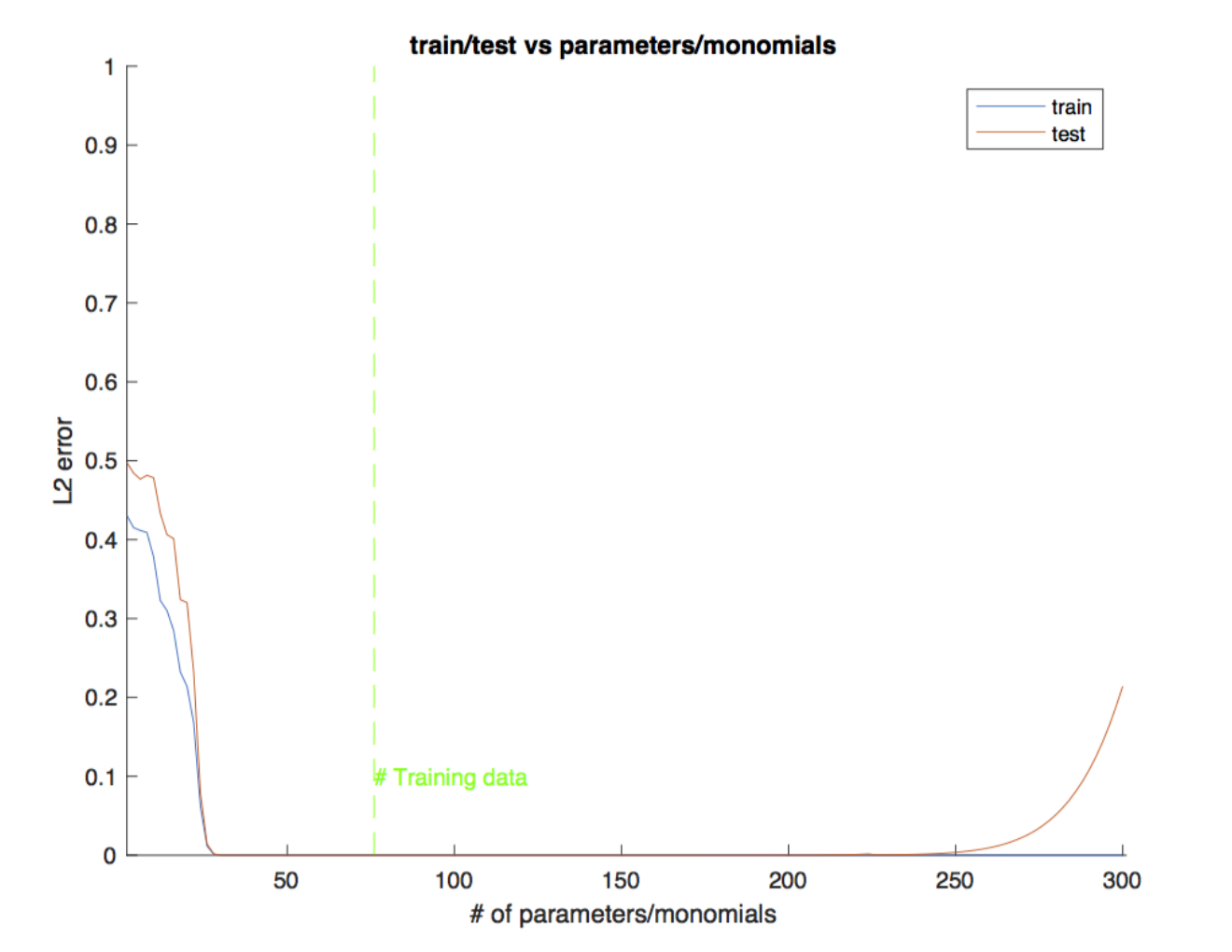
This is only part of the explanation. With real data there is always some “noise”, either in the training or testing data, since they do not exactly reflect the “true” underlying distribution. This implies the usual appearance of small overfitting. This is the case for the right side of Figure 2. The classification error is more resistant to overfitting, if the data satisfy Tsybakov “low noise” conditions (data density is low at the classification boundary). This explains the behavior of the left side of Figure 2, despite the small overfitting of the cross-entropy loss (on the right).
10 Hartman-Grobman theorem and dynamical systems
Consider the case in which the stable point(s) of the dynamical system is hyperbolic (the eigenvalues of the associated Hessian are negative). In this case the Hartman-Grobman theorem ([22]) holds (recall we assume that the RELUs are smoothly differentiable, since they can be replaced by polynomials). It says that the behavior of a dynamical system in a domain near a hyperbolic equilibrium point is qualitatively the same as the behavior of its linearization near this equilibrium point. Here is a version of the theorem adapted to our case.
Hartman-Grobman Theorem Consider a system evolving in time as with a smooth map . If has a hyperbolic equilibrium state and the Jacobian of at has no zero eigenvalues, then there exist a neighborhood of and a homeomorphism , s.t. and in the flow of is topologically conjugate by the continuous map to the flow of the linearized system where is the Hessian of .
Flows
For a linear dynamical system , we can define the flow of the solutions , which is the collection of the solutions depending on the initial conditions. The flow is solved by
| (9) |
Note, that for a symmetric matrix , all that really matters for the dynamics are the eigenvalues of , since we can perform the diagonalization , where is a diagonal matrix of eigenvalues of and is an orthogonal matrix. We can then write
Now is just a rotation or reflection in , so up to this simple transformation, the dynamics of a linear system and its phase portrait are governed by the eigenvalues of A.
Conjugacy
An important question in the theory of dynamical systems is whether any two given systems are different from each other. There exists several notions of equivalence, differing in smoothness. Here we review three of them:
- 1.
Linear conjugacy We say that two linear systems and are linearly conjugate iff there exists an invertible transformation such that and . Linear conjugacy is thus equivalent to similarity of matrices.
- 2.
Differentiable conjugacy For nonlinear systems, we can consider nonlinear changes of coordinates , where is a diffeomorphism, i.e. a continuously differentiable bijective map with a continuously differentiable inverse. We then say that an equation on some open set is differentiably conjugate to on when there exists a diffeomorphism such that the change of variables converts one of the systems to the other. The requirement for this to happen is
(10) Around equilibria and of the two dynamical systems, the dynamics linearize to
(11) and the two systems are linearly conjugate by . This implies that, like in the linear case, the eigenvalues of and have to be the same.
- 3.
Topological conjugacy A relaxation of the above employs homeomorphisms (continuous bijective maps with continuous inverse) rather than diffeomorphisms. We say that two flows of dynamical systems and are topologically conjugate if there exists a homeomorphism such that we have
(12) Importantly, for linearized systems with flows and the topological conjugacy relaxes the statement of similarity of and to the requirement that the dimensions of stable and unstable spaces of are equal to those of , i.e. only the signs of eigenvalues have to match.
11 Analysis: One layer linear networks
In this section we prove existence of a finite limit for the normalized weight vector independently of initial conditions. Our approach uses dynamical systems tools. It is more qualitative and less detailed than [1] but it can be used also for the nonlinear case in section 12.
We consider linear networks with one layer and one scalar output with (multilayer linear networks have been recently analyzed by [23]).
11.1 Square loss
Consider
| (13) |
where is a bounded real-valued variable. Assume further that the -dimensional weight vector fits all the training data, achieving zero loss on the training set, that is
- 1.
Dynamics The dynamics is
(14) with .
The only components of the the weights that change under the dynamics are in the vector space spanned by the examples ; components of the weights in the null space of the matrix of examples are invariant to the dynamics. Thus converges to the minimum norm solution if the dynamical system starts from zero weights, as we will see also later.
- 2.
Linearized dynamics The Jacobian of – and Hessian of – for is
(15) This linearization of the dynamics around for which yields
(16) where the associated is convex, since the Jacobian is minus the sum of auto-covariance matrices and thus is semi-negative definite. It is negative definite if the examples span the whole space but it is degenerate with some zero eigenvalues if [11].
- 3.
Regularization If a regularization term is added to the loss the gradient will be zero for finite values of .
In detail we have
(17) with
(18) which is always negative definite for any arbitrarily small . Thus the equilibrium in
(19) is hyperbolic and the Hartman-Grobman theorem applies.
In summary, regularization ensures the existence of a hyperbolic equilibrium for any at a finite (which increases to for ). If the initial conditions are , in the limit of the equilibrium converges to a minimum norm solution for and a maximum margin solution for . The reason is that the degenerate directions of in which the gradient is zero will not change during gradient descent and remain close to .
11.2 Exponential loss
Consider now the exponential loss. Even for a linear network the dynamical system associated with the exponential loss is nonlinear. While [1] gives a rather complete characterization of the dynamics, here we describe a different approach based on linearization of the dynamics. We will then extend this analysis from linear networks to nonlinear networks.
The exponential loss is
| (20) |
where is a binary variable taking the value or . Assume further that the -dimensional weight vector separates correctly all the training data, achieving zero classification error on the training set, that is . In some cases below (it will be clear from context) we incorporate into .
- 1.
Dynamics The dynamics is
(21) thus .
It is well-known that the weights of the networks that change under the dynamics must be in the vector space spanned by the examples ; components of the weights in the null space of the matrix of examples are invariant to the dynamics, exactly as in the square loss case. Unlike the square loss case, the dynamics of the weights diverges but the limit is finite and defines the classifier. This means that if a few components of the gradient are zero (for instance when the matrix of the examples is not full rank – which is the case if ) the associated component of the vector will not change anymore and the corresponding component in will be zero. This is why there is no dependence on initial conditions, unlike the square loss case.
- 2.
Linearized dynamics Though there are no equilibrium points at any finite , we can look at the Jacobian of – and Hessian of – for a large but finite . It is
(22) The linearization of the dynamics around any finite yields a convex , since is the negative sum of auto-covariance matrices. The Jacobian is semi-negative definite in general. It is negative definite if the examples span the whole space but it is degenerate with some zero eigenvalues if .
The dynamics of perturbation around is given by
(23) where the degenerate directions of the gradient will be washed out asymptotically in the vector which is effectively used for classification, as described earlier.
- 3.
Regularization If an arbitrarily small regularization term such as is added to the loss, the gradient will be zero for finite values of – as in the case of the square loss. Different components of the gradient will be zero for different v . At this equilibrium point the dynamic is hyperbolic and the Hartman-Grobman theorem directly applies:
(24) The minimum is given by , which can be solved by with for .
The Hessian of in the linear case for s.t. is given by
(25) which is always negative definite, since it is the negative sum of the coefficients of positive semi-definite auto-covariance matrices and . This means that the minimum of is hyperbolic and linearization gives the correct behavior for the nonlinear dynamical system.
As before for the square loss, regularization ensures the existence of a hyperbolic equilibrium. In this case the equilibrium exists for any at a finite which increases to for . In the limit of the equilibrium converges to a maximum margin solution for . The reason is that the components of in which the gradient is zero will not change during gradient descent. Those components will be divided by a very large number (the norm of ) and become zero in the normalized norm .
12 Analysis: Nonlinear deep networks
12.1 Square loss
| (26) |
Here we assume that the function achieves zero loss on the training set, that is
- 1.
Dynamics
The dynamics now is
(27) with .
- 2.
Linearized dynamics The Jacobian of – and Hessian of – for is
(28) where the last step is because of . Note that the Hessian involves derivatives across different layers, which introduces interactions between perturbations at layers and . The linearization of the dynamics around for which yields a convex , since the Jacobian is semi-negative definite. In general we expect several zero eigenvalues because the Hessian of a deep overparametrized network under the square loss is degenerate as shown by the following theorem in Appendix 6.2.4 of [11]:
Theorem 4
(K. Takeuchi) Let be a positive integer. Let for and , where . Consider a set of -hidden layer models of the form, parameterized by . Let be the objective function. Let be any twice differentiable point of such that . Then, if there exists such that where and (i.e., overparametrization), there exists a zero eigenvalue of Hessian .
- 3.
Regularization The effect of regularization is to add the term to the loss. This results in a Hessian of the form
(29)
which is always negative definite for any .
12.2 Exponential loss
Consider again the exponential loss
| (30) |
with definitions as before. We assume that , parametrized by the weight vectors , separates correctly all the training data , achieving zero classification error on the training set for , that is . Observe that if separates the data, then and this is where gradient descent converges [1].
Again there is no critical point for finite . Let us linearize the dynamics around a large by approximating with a low order Taylor approximation for small .
- 1.
Dynamics
The gradient flow is not zero at any finite . It is given by
(31) where the partial derivatives of w.r.t. can be evaluated in .
Let us consider a small perturbation of around in order to linearize around .
- 2.
Linearized dynamics
The linearized dynamics of the perturbation are , with
(32) Note now that the term containing the second derivative of does not vanish at a minimum, unlike in the square loss case. Indeed, away from the minimum this term contributes negative eigenvalues.
- 3.
Regularization
Adding a regularization term of the form yields for
(33) For compactness of notation, let us define
(34) with which we have a transcendental equation for the minimum.
(35) The Jacobian of (and negative Hessian of loss) is then
(36) - 4.
At this new finite equilibrium the Hessian is now positive definite for any . This guarantees that a perturbation around remains small: there is asymptotic stability. Furthermore, for the exponential loss – but not for the square loss – the dynamics for any close to remains qualitatively the same when , in other words is not affected by the presence of regularization. The parameters resulting from linearization may be different from the original weights: the minimum norm solution is in terms of these new local parameters.
- 5.
Normalized dynamics
We consider here the dynamics of the normalized network with normalized weight matrices induced by the gradient dynamics of , where is the weight matrix of layer . We note that this normalized dynamics is related to the technique called “weight normalization” used in gradient descent[24]. For simplicity of notation we consider here for each weight matrix the corresponding “vectorized” representation in terms of a vector that we denote as (dropping the index for convenience).
We use the following definitions and self-evident properties:
- •
Define ; thus with .
- •
The following relations are easy to check:
- (a)
- (b)
. has at most one zero eigenvalue since is rank with a single eigenvalue .
- (c)
- (d)
- (e)
- (a)
- •
We assume .
- •
Thus
- •
The gradient descent dynamic system used in training deep networks for the exponential loss of Equation 30 is given by Equation 6, that is by
(37) with a Hessian given by (assuming )
(38) - •
The dynamics above for induces the following dynamics for and :
(39) and
(40) Thus
(41) where, assuming that is the vector corresponding to the weight matrix of layer , we obtain because of Lemma 1 in [10]. We assume that separates all the data, that is . Thus and . In the 1-layer network case the dynamics yields asymptotically. For deeper networks, this is different. In Section 14 we show that the product of weights at each layer diverges faster than logarithmically, but each individual layer diverges slower than in the 1-layer case. By defining
(42) the Equation above becomes
(43) The dynamics imply for , while . As in the square loss case for , the degenerate components of are not directly updated by the gradient equation but unlike the square loss case, they are indirectly updated because . Thus the dynamics is independent of the initial conditions, unlike the dynamics of in the square loss case. Note that the constraint is automatically enforced by the definition of .
- •
This section, and in particular inspection of Equations 41 and 43, shows that the dynamics of the normalized matrices at each layer converges. Adding a regularization term of the form and letting go to supports the following conjecture
Proposition 5
The normalized weight matrix at each layer converges to the minimum Frobenius norm solution, independently of initial conditions.
12.3 Another approach to prove linearization of a nonlinear deep network and its validity
In this section we study the linearization of the deep nonlinear networks around fixed points of GD and its relation with equivalent linear networks. We first review the step of linearization described in section 5.1 for linear networks with either square or exponential losses to study the dynamics of perturbations . We also review the same linearizaton step for the deep nonlinear networks. Unlike the linear case, the Hessian can have negative eigenvalues, and only becomes positive-definite around the minimum.
We then
- •
show that in the case of the square loss, the Hessian of a deep nonlinear network can be mapped to a linear network with appropriately transformed data;
- •
for the exponential losses we show that linearization of a deep nonlinear network yields a deep linear network.
- •
show that the Hartman-Grobman theorem guarantees that the linearization faithfully describes the behavior of the DNNs near a minimum of GD.
Proof sketch
We first regularize the square loss or a loss with an exponential tail and derive the continuous dynamical system in associated with gradient descent (with a fixed learning rate). We then linearize around the asymptotic equilibrium at which the gradient is zero, obtaining the dynamical system for perturbations around in Equation (5). At this point we check that the analysis available for linear networks – especially in the case of exponential losses – applies to the linearized dynamical systems. For this, we need to understand the dynamics of perturbations for both the linear networks and the deep nonlinear ones.
Note that the phase portraits of a dynamical system (5) depend solely on the eigenvalues of . For both the exponential losses and the square loss on linear networks, the Hessian is positive semi-definite everywhere, even without any regularization, with the number of distinct eigenvalues bounded by – the number of training examples . For the deep nonlinear networks, the Hessian can in general have negative eigenvalues, and only at a minimum of GD it become positive semi-definite. Interestingly, for the square loss at the Hessian has also at most distinct eigenvalues, since we have
where vanishes at a zero minimum. Due to the higher number of weights than in the one layer linear network case, the Hessian is of higher dimensionality () than in the linear case (). This implies that the linearization of the nonlinear deep network with square loss corresponds to a linear system with higher dimensional “virtual” data related to the original data by . This construction provides a (stronger) differentiable conjugacy to a linear network.
In the case of losses with exponential tails, the Hessian has a non-vanishing additional term proportional to . In the case of the exponential loss we obtain
In particular, derivatives across different layers induce a higher number of distinct eigenvalues than . We show below that deep linear networks (with ) have the same behavior for derivatives across layers (here and elsewhere we do not assume a convolutional structure). The only difficulty is then of two derivatives in the same layer, , which we remove by the assumption of rectified nonlinearities, for which the second derivative vanishes. Thus a deep nonlinear network with an exponential loss linearizes to a deep linear network with same loss, which also converges to the pseudo-inverse like the shallow linear network. Finally, the linearized system satisfies the Hartman-Grobman theorem (for any ) and is therefore a good qualitative description of the dynamics of the nonlinear system around the asymptotic equilibrium .
12.3.1 Square loss
Note that the Hessian of a deep network is of much higher dimensionality for over-parametrized networks. However, since the number of distinct eigenvalues of the linear and nonlinear Hessians match (since they are both sums of outer products of training example vectors), we can find a linear system with inputs with and weights that satisfies the same linearized dynamical system as the linearized deep network. Since we can explicitly match the two Hessians, the dynamical system of a deep network with a square loss around a minimum of gradient descent is differentiably conjugate to a linear network with square loss.
12.3.2 Exponential loss
The Hessian around for the exponential loss is quite different from the square loss case for the same network . This is because the term cannot in general be written as an outer product of some vector. Let us investigate two simple cases.
- 1.
Consider a simple one-layer network, with an arbitrary smooth non-linear activation applied to it. In this case we have . It is easy to see that in this case
(44) which is again a simple outer product of a vector. Hence, the Hessian has again at most distinct eigenvalues, just like in the linear case. It is interesting to note that this simple case is also valid for a deep network, if we restrict ourselves to optimizing only one layer at a time. This extends the results in [1] from piecewise-linear activations to arbitrary nonlinear smooth ones.
In the one-layer case there exists a simple mapping of the continuum GD dynamics of the nonlinear network around a minimum to an equivalent linear system with an exponential loss by setting . The exact mapping of Hessians implies again a differentiable conjugacy of the two dynamical systems.
- 2.
If we add a single linear layer on top of the one we just considered, i.e. , the second derivative becomes
(45) The second term here cannot be written as a simple outer product of a vector, hence there is no guarantee that the Hessian has only distinct eigenvalues. This naturally extends to the case with more layers. Indeed, simple numerical checks show that this bound is generically broken.
From the second example it is clear that when we consider derivatives across layers, the Hessian of a deep network with an exponential loss around a minimum for training examples has more eigenvalues than a one layer linear model with the same loss. Adding a regularization term helps with making all the eigenvalues positive, but does not change the number of distinct eigenvalues. Hence, unlike the square loss, there does not exist a linear model with a single layer which is differentiably conjugate to the dynamical system of the deep network around a minimum. Nonetheless, after adding an arbitrarily small regularization it is possible to construct a linear network with an equal number of positive eigenvalues. Thus the dynamical system of a deep nonlinear network with arbitrarily small regularization parameter around a minimum of gradient descent is topologically conjugate to that of a regularized linear network.
It is natural to ask whether we can strengthen this statement into differentiable conjugacy in some way. With this in mind, let us consider a deep linear network, which also converges in general to the minimum norm solution. We have for a network with layers. Without loss of generality, consider the two-layer case, for which the Hessian is
| (46) |
This expression clearly cannot be written as a sum of outer products of vectors, hence we expect it to have in principle more than distinct eigenvalues. This is indeed generically true in simulations.
We would like to compare this to the Hessian of a nonlinear deep network
where the second term is given by Equation (45). To simplify the comparison, let us consider case when the second derivative at the same layer vanishes, which holds true for rectified nonlinearities. The nonlinear network can be written as , where is a diagonal matrix with entries 0 or 1 giving the profile of the ReLU activations in layer [10]. While it is straightforward to match the value of the nonlinear network to a linear one at a point for each of the training examples, we do not in principle have enough variables to match the Hessians exactly. From the discussion in Section 10 we know that we only have to match the eigenvalues, rather than matrices. In [25] the spectrum of the Hessian of a deep network with cross-entropy loss was studied numerically and was shown to be highly degenerate around a minimum of GD.
Since the Hessians are real symmetric matrices, they are linearly conjugate to diagonal matrices. Thus we obtain two linear systems and , where and are the eigenvalues of the nonlinear and linear deep networks respectively. Adding an arbitrarily small regularization now gives hyperbolic dynamics, for which the Hartman-Grobman theorem applies. Ordering the eigenvalues so that and similarly for , we can construct the conjugacies
| (47) |
If , then is a diffeomorphism, otherwise it is a homeomorphism. If there exists a deep linear network with the same number of distinct eigenvalues as the nonlinear one at a minimum (up to the freedom of choosing the regularization parameters), then we obtain differentiable conjugacy. Otherwise there will exist directions in weight-space in which the equivalence will hold up to a topological conjugacy. Whether the number of eigenvalues can be matched remains an open question.
The results above hold not only for the exponential loss, but also for the family of losses with exponential tails, for example the logistic function. Note that technically the statements above work for smooth nonlinearities, for example , but we expect they should apply to non-smooth dynamical systems in the Filippov sense [15].
In particular, the results obtained by [1] and [23] for the case of linear networks (both shallow and deep) guarantee a “linearized” minimum norm solution in the neighborhood of independently of the path taken by gradient descent to reach the neighborhood of . In our derivation this is because the convergence is driven by non zero gradient and it is thus independent of initial conditions. It is important to note that this situation is unlike the case of the square loss (see Figure 3) where the dependence on initial conditions means that the norm of the local linearized solution depends on the overall trajectory of gradient descent and not only on .
13 Early stopping
We discuss here a slightly different dynamical system minimizing the same exponential loss function. The dynamics is related to gradient descent with batch normalization.
Consider the usual loss function . We define for where is the number of layer and is the matrix of weights of layer , is the normalized matrix of weights at layer . Homogeneity of implies . We enforce as constraints (any constant instead of is acceptable) in the minimization of by penalization controlled by . Note that this penalty is formally different from a regularization parameter since it enforces unit norm. Thus we are led to finding and for which is zero. We minimize with respect to by gradient descent. We obtain for
| (48) |
and for each layer
| (49) |
where .
Observe (see next section) that , decreasing to zero for . Also from the results in Section 14. Note that, since , Equation 49 implies
| (50) |
Equation 50 can be rewritten as
| (51) |
with decreasing to zero for increasing . When the equilibrium is reached and has unit norm.
In the approach of this section the values of the are set by which enforces the constraint. This means that the value of effectively determines , the time at which the change in stop because . Thus a finite stopping time follows from the value of . The dynamics around the equilibrium point is hyperbolic for any , allowing the use of the Hartman-Grobman theorem. Note that the unperturbed dynamics around is topologically the same for as well as for . This suggests a possible approach to prove that (necessary) early stopping is equivalent to regularization. The argument would claim that in the absence of the terms the dynamics has to be stopped after a (possibly very long) time and this is equivalent to a small finite regularization term.
Finally, the Hessian of wrt tells us about the linearized dynamics around a minimum where the gradient is zero. The Hessian is
| (52) |
Thus the Hessian is negative semidefinite for for large times because the absolute value of the first term decreases more slowly than the second term. However, it is asymptotically negative definite with any and thus also in the limit of .
Putting together all the observations above we have the following proposition:
Proposition 6
The linearized dynamics for the exponential loss is hyperbolic for large, finite , describing the dynamics of each layer weight matrix near a zero minimum of the loss. The Hartman-Grobman theorem implies that near a global asymptotic minimum , for an arbitrarily large finite , the linearized flow is topologically equivalent to the nonlinear dynamics induced by a deep network. The flow converges to the local maximum margin solution asymptotically, independently of the trajectory leading to the global minimum.
Remarks
The intuition behind the equations of this section is that if a solution for the weights exists such that , then the normalized solution also separates the data. In this case the loss can be made as small as desired by increasing . Among all normalized solutions, GD selects the one with minimum norm because only the nondegenerate directions around a minimum – in which the gradient is not zero – increase. The degenerate directions, which do not change, are “washed out” by normalization since the effective norm increases steadily during gradient descent. This justifies the term and its limit for .
Note that we do not assume linearization in the previous paragraph. Linearization only enters when we consider the Hessian and its properties around a minimum. It seems therefore possible to compare meaningfully the norms of different minima to predict expected errors. In particular, consider running gradient descent. Assume that GD converges to an asymptotic global minimum, around which the increase in the norm is very slow. Set and use Equations 48, 49, with , to compute the products of the Frobenius norms when . This network norm would be a proxy for the complexity of the network at the specific minimum, allowing a comparison of different minimizers.
14 Rate of growth of weights
In linear 1-layer networks the dynamics of gradient descent yield asymptotically. For the validity of the results in the previous section, we need to show that the weights of a deep network also diverge at infinity. In general, the nonlinearly coupled equations (48) are not easily solved analytically. For simplicity of analysis, let us consider the case of a single training example , as we expect the leading asymptotic behavior to be independent of . In this regime we have
| (53) |
Keeping all the layers independent makes it difficult to disentangle for example the behavior of the product of weights , as even in the 2-layer case the best we can do is to change variables to and , for which we still get the coupled system
| (54) |
from which reading off the asymptotic behavior is nontrivial.
As a simplifying assumption let us consider the case when . This gives us the single differential equation
| (55) |
This implies that for the exponentiated product of weights we have
| (56) |
Changing the variable to , we get finally
| (57) |
We can now readily check that for we get , so . It is also immediately clear that for the product of weights diverges faster than logarithmically. In the case of we get , where is the logarithmic integral function. We show a comparison of the 1-layer and 2-layer behavior in the left graph in Figure 7. For larger we get faster divergence, with the limit given by , where and .
Interestingly, while the product of weights scales faster than logarithmically, the weights at each layer diverge slower than in the linear network case, as can be seen in the right graph in Figure 7.
Remarks
- •
Cross-entropy loss with Softmax classifier While the results in the article have been derived for binary classification, they extend to the case of labels in the set . In this case we can write the neural network with layers and rectified nonlinearities as
(58) where the last layer . In this notation is a -dimensional vector and we can label its’ -th component as . The cross-entropy loss with the Softmax classifier is then
(59) where is the component of corresponding to the correct label for the example . The gradient of the loss is then
(60) The equivalent assumption of non-linear separability for the cross-entropy loss is that there exists a such that . Using the property of rectified networks , we immediately get that
for any value of . We thus get that as the gradient of the cross-entropy loss , the weights diverge. Rewriting we see that up to a slightly different normalization (by a sum of exponentials rather than a single exponential) and an additional summation, the dynamics of GD for the cross-entropy loss are those of the exponential loss for binary classification, and as such the results in this article apply also to multi-class classification.
- •
GD with weight normalization Note that the dynamics of Equations 48 and 49 is different from other gradient descent dynamics, though similar. It represents one of the possible approaches for training deep nets on exponential type losses: the first approach is to update and then, in principle at least, normalize at the end. The second approach, is similar to using weight normalization: GD implements the dynamics of . The third approach uses the dynamics corresponding to a penalization term enforcing unit Frobenius norm of the weight matrix .
- •
Non separable case Consider the linear network in the exponential loss case. There will be a finite for which the gradient is zero. The question is whether this is similar to the regularization case or not, that is whether misclassification regularizes.
Let us look at a linear example:
(61) in which we assume that there is one classification error (say for ), meaning that the term grows exponentially with . Let us also assume that gradient descent converges to . This implies that : for the gradient is zero and . Is this a hyperbolic equilibrium? Let us look at a very simple , case:
(62) If then for which implies . This is clearly a hyperbolic equilibrium point, since we have
(63) so the single eigenvalue in this case has no zero real part.
In general, if there are only a small number of classification errors, one expects a similar situation for some of the components. Differently from the regularization case, misclassification errors do not “regularize” all components of but only the ones in the span of the misclassified examples.
- •
Learning rate and discretization In the paper we have neglected the time dependence of the learning rate in GD because we considered the associated continuous dynamical systems. A time-dependent learning rate is important when the differential equations are discretized. This can be seen by considering the differential equation
(64) with solution . The condition corresponds to . Conditions of this type are needed for asymptotic convergence to the minimum of the process . Consider now the “noisy” case : we need to eliminate the effect the “noise” , implying at least . The “noise” may just consist of discretization “noise”.
References
- [1] D. Soudry, E. Hoffer, and N. Srebro. The Implicit Bias of Gradient Descent on Separable Data. ArXiv e-prints, October 2017.
- [2] Moritz Hardt and Tengyu Ma. Identity matters in deep learning. CoRR, abs/1611.04231, 2016.
- [3] Behnam Neyshabur, Srinadh Bhojanapalli, David McAllester, and Nathan Srebro. Exploring generalization in deep learning. arXiv:1706.08947, 2017.
- [4] Jure Sokolic, Raja Giryes, Guillermo Sapiro, and Miguel Rodrigues. Robust large margin deep neural networks. arXiv:1605.08254, 2017.
- [5] P. Bartlett, D. J. Foster, and M. Telgarsky. Spectrally-normalized margin bounds for neural networks. ArXiv e-prints, June 2017.
- [6] C. Zhang, Q. Liao, A. Rakhlin, K. Sridharan, B. Miranda, N.Golowich, and T. Poggio. Musings on deep learning: Optimization properties of SGD. CBMM Memo No. 067, 2017.
- [7] L. Rosasco and B. Recht. Waiting for godot. CBMM Memo 0XY, 2017. Regression part only orally disclosed before writing this paper.
- [8] M. Anthony and P. Bartlett. Neural Network Learning - Theoretical Foundations. Cambridge University Press, 2002.
- [9] Moritz Hardt, Benjamin Recht, and Yoram Singer. Train faster, generalize better: Stability of stochastic gradient descent. CoRR, abs/1509.01240, 2015.
- [10] Tengyuan Liang, Tomaso Poggio, Alexander Rakhlin, and James Stokes. Fisher-rao metric, geometry, and complexity of neural networks. CoRR, abs/1711.01530, 2017.
- [11] T. Poggio, Q. Liao, B. Miranda, L. Rosasco, X. Boix, J. Hidary, and H. Mhaskar. Theory of deep learning III: explaining the non-overfitting puzzle. arXiv:1703.09833, CBMM Memo No. 073, 2017.
- [12] Chiyuan Zhang, Samy Bengio, Moritz Hardt, Benjamin Recht, and Oriol Vinyals. Understanding deep learning requires rethinking generalization. CoRR, abs/1611.03530, 2016.
- [13] Yuan Yao, Lorenzo Rosasco, and Andrea Caponnetto. On early stopping in gradient descent learning. Constructive Approximation, 26(2):289–315, Aug 2007.
- [14] N.P. Bhatia and G.P. Szegö. Stability Theory of Dynamical Systems. Classics in Mathematics. Springer Berlin Heidelberg, 2002.
- [15] F.M. Arscott and A.F. Filippov. Differential Equations with Discontinuous Righthand Sides: Control Systems. Mathematics and its Applications. Springer Netherlands, 1988.
- [16] C. Zhang, Q. Liao, A. Rakhlin, K. Sridharan, B. Miranda, N.Golowich, and T. Poggio. Theory of deep learning IIb: Optimization properties of SGD. CBMM Memo 072, 2017.
- [17] A Krizhevsky. Learning multiple layers of features from tiny images. Technical Report, 2009.
- [18] T. Poggio and Q. Liao. Theory II: Landscape of the empirical risk in deep learning. arXiv:1703.09833, CBMM Memo No. 066, 2017.
- [19] M. Belkin, S. Ma, and S. Mandal. To understand deep learning we need to understand kernel learning. ArXiv e-prints, Feb 2018.
- [20] T. Poggio, H. Mhaskar, L. Rosasco, B. Miranda, and Q. Liao. Theory I: Why and when can deep - but not shallow - networks avoid the curse of dimensionality. Technical report, CBMM Memo No. 058, MIT Center for Brains, Minds and Machines, 2016.
- [21] H.N. Mhaskar and T. Poggio. Deep vs. shallow networks: An approximation theory perspective. Analysis and Applications, pages 829– 848, 2016.
- [22] Thomas Wanner. The hartman-grobman theorem for caratheodory-type differential equations in banach spaces. 2000.
- [23] S. Gunasekar, J. Lee, D. Soudry, and N. Srebro. Implicit Bias of Gradient Descent on Linear Convolutional Networks. ArXiv e-prints, June 2018.
- [24] Tim Salimans and P. Kingma Diederik. Weight normalization: A simple reparameterization to accelerate training of deep neural networks. Advances in Neural Information Processing Systems, 2016.
- [25] Levent Sagun, Léon Bottou, and Yann LeCun. Singularity of the hessian in deep learning. CoRR, abs/1611.07476, 2016.