跳到论文正文
W Papers独立论文阅读器 arXiv:1806.11057 论文正文 计算阅读时间 · 0%
引用这篇论文根据当前论文元数据生成,正式投稿前建议核对。


License: arXiv.org perpetual non-exclusive license
arXiv:1806.11057v1 [physics.plasm-ph] 28 Jun 2018

The electric field of an electron in a electron-hole plasma with degenerate electrons

S. P. Sadykova1    A. A. Rukhadze2 Affiliation: 1 Forschungszentrum Julich, Jülich Supercomputing Center, Jülich, Germany
2 Prokhorov General Physics Institute, Russian Academy of Sciences, Moscow, Russia
Abstract

We consider the possibility of formation of a superconductivity state either in a semiconductor or in a electron-hole plasma with the degenerate electrons due to the attractive forces between the electrons as a result of the exchange effects through the electron-hole sound wave by analogy to the phonon waves in a solid state. We have determined the view of an interaction potential between two electrons in a degenerate electron-hole plasma. The potential appears to be attractive at distances large than the Debye radius and decreases as 1/r31/r^{3}. We discuss the conditions at which the bound electron state - Cooper Pair in a such field can be formed.

1 Introduction

Here we would like to consider the conditions for existence of the electron-hole sound waves in a semiconductor at cryogenic temperatures when electrons (light and of a negative charge) are degenerate and one of the major unsolved problems of the superconductivity theory is determination of the static potential of a point electron. Obviously, the sign of the electron potential in a superconductive medium must be opposite to that in a vacuum. This follows from the Bardeen-Cooper-Schrieffer theory, since the Cooper electron pair can form only when the potential appears to be attractive for both electrons. Below, we will show that in a electron-hole plasma of a semiconductor when the electrons are degenerate and holes are not degenerate, i.e. when

ϵF−=PF−22​m−=3​π22/3​ℏ2​n−2/32​m−>>kB​T−≥kB​T+>>3​π22/3​ℏ2​n+2/32​m+,{\epsilon_{F-}}=\frac{P_{F-}^{2}}{2m_{-}}=\frac{{3\pi^{2}}^{2/3}\hbar^{2}{n_{-}}^{2/3}}{2m_{-}}>>k_{B}T_{-}\geq k_{B}T_{+}>>\frac{{3\pi^{2}}^{2/3}\hbar^{2}{n_{+}}^{2/3}}{2m_{+}}, (1)

a weakly damped electron-hole sound wave with the speed

VF−=2​ϵF−m−>>vs=ϵF−3​m+>>VT+=kB​Tm+{V_{F-}}=\sqrt{\frac{2\epsilon_{F-}}{m_{-}}}>>v_{s}=\sqrt{\frac{\epsilon_{F-}}{3m_{+}}}>>{V_{T+}}=\sqrt{\frac{k_{B}T}{m_{+}}} (2)

can form in such a plasma . The electron-hole sound wave can be described by the following dispersion relation [1].

ϵl​(ω,k)=1+3​ωL−2k2​VF−2​(1+ı​π​ω2​k​VF−)−ωL+2ω2=0.{\epsilon^{l}(\omega,k)}=1+\frac{3\omega_{L-}^{2}}{k^{2}V_{F-}^{2}}(1+\imath\frac{\pi\omega}{2kV_{F-}})-\frac{\omega_{L+}^{2}}{\omega^{2}}=0. (3)

where the following oscillation spectrum comes from:

ω2=ωL+21+3​ωL−2/k2​VF−2,δ=−34​π​m+m−​ωL+4k3​VF−3.\omega^{2}=\frac{\omega_{L+}^{2}}{1+3\omega_{L-}^{2}/k^{2}V_{F-}^{2}},\>\>\>\>\>\delta=-\frac{3}{4}\frac{\pi m_{+}}{m_{-}}\frac{\omega_{L+}^{4}}{k^{3}V_{F-}^{3}}. (4)

In a long range limit at 3​ωL−2>>k2​VF−23\omega_{L-}^{2}>>k^{2}V_{F-}^{2} or

k2​rD2=k2​VF−23​ωL−2<<1.k^{2}r_{D}^{2}=k^{2}\frac{V_{F-}^{2}}{3\omega_{L-}^{2}}<<1. (5)

Taking into account that n−=n+n_{-}=n_{+}, we can get the linear spectrum from .

ω=k​n+3​n−​m−m+​VF−,δ=−π4​n+n−​n+3​n−​m−m+​ω.\omega=k\sqrt{\frac{n_{+}}{3n_{-}}\frac{m_{-}}{m_{+}}}V_{F-},\>\>\>\>\>\delta=-\frac{\pi}{4}\frac{n_{+}}{n_{-}}\sqrt{\frac{n_{+}}{3n_{-}}\frac{m_{-}}{m_{+}}}\omega. (6)

In a short range limit, when the inverse to relation is satisfied, we get

ω2=ωL+2,δ=−34​π​m+m−​ωL+2k3​VF−3.\omega^{2}=\omega_{L+}^{2},\>\>\>\>\>\delta=-\frac{3}{4}\frac{\pi m_{+}}{m_{-}}\frac{\omega_{L+}^{2}}{k^{3}V_{F-}^{3}}. (7)

2 The interaction potential of two electrons in a electron-hole plasma

The interaction potential of two electrons α\alpha and β\beta in a electron-hole plasma can be described by the following equation [2]:

U⁡(r)=∫eı​k→​r→​U​(k→)​𝑑k→,U⁡(k)=eα​eβ2​π2​1k2​εl​(k​Vα,k).U(r)=\int e^{\imath\vec{k}\vec{r}}U(\vec{k})d\vec{k},\>\>\>\ U(k)=\frac{e_{\alpha}e_{\beta}}{2\pi^{2}}\frac{1}{k^{2}\varepsilon^{l}(kV_{\alpha},k)}. (8)

According to the Eq. (ref3)

k2​ϵl​(k​Vα,k)=k2+3​ωL−2VF−2−ωL+2Vα2+ı​β,β=3​π​Vα​ωL−2VF−3,k^{2}{\epsilon^{l}(kV_{\alpha},k)}=k^{2}+\frac{3\omega_{L-}^{2}}{V_{F-}^{2}}-\frac{\omega_{L+}^{2}}{V_{\alpha}^{2}}+\imath\beta,\>\>\>\beta=\frac{3\pi V_{\alpha}\omega_{L-}^{2}}{V_{F-}^{3}}, (9)

here VαV_{\alpha} is the speed of a test electron with the charge eαe_{\alpha} producing the potential ϕα\phi_{\alpha} at a point r=0r=0 where the charge eβe_{\beta} is located. Taking into account that d​r→/d​t=Vαd\vec{r}/dt=V_{\alpha}, it follows r→↑↑Vα\vec{r}\uparrow\uparrow V_{\alpha}, Vα>VT+V_{\alpha}>V_{T+}. As a result, at eα=eβ=ee_{\alpha}=e_{\beta}=e we will get

U⁡(k)=e22​π2​1k2+3​ωL−2VF−2−ωL+2Vα2​x2+ı​β,U⁡(r)=e22​π2​∫eı​k​r​x​d​k→k2+3​ωL−2VF−2−ωL+2Vα2​x2+ı​β,U(k)=\frac{e^{2}}{2\pi^{2}}\frac{1}{k^{2}+\frac{3\omega_{L-}^{2}}{V_{F-}^{2}}-\frac{\omega_{L+}^{2}}{V_{\alpha}^{2}x^{2}}+\imath\beta},\>\>\>\ U(r)=\frac{e^{2}}{2\pi^{2}}\int\frac{e^{\imath krx}d\vec{k}}{k^{2}+\frac{3\omega_{L-}^{2}}{V_{F-}^{2}}-\frac{\omega_{L+}^{2}}{V_{\alpha}^{2}x^{2}}+\imath\beta}, (10)

where x=c​o​s​(θ)x=cos(\theta).
Let us analyse this expression in two limitting cases: 1) In a short range limit at r∼1k≤VF−ωL−<<VαωL+∼VF−ωL+r\sim\frac{1}{k}\leq\frac{V_{F-}}{\omega_{L-}}<<\frac{V_{\alpha}}{\omega_{L+}}\sim\frac{V_{F-}}{\omega_{L+}} 2) In a long range limit at r∼1k>>VF−ωL−r\sim\frac{1}{k}>>\frac{V_{F-}}{\omega_{L-}}.

2.1 The short range limit interaction

U(r)=e22​π2∫eı​k→​r→​d​k→k2+1rD−2=e2re−r/rD−,U(r)=\frac{e^{2}}{2\pi^{2}}\int\frac{e^{\imath\vec{k}\vec{r}}d\vec{k}}{k^{2}+\frac{1}{r_{D-}^{2}}}=\frac{e^{2}}{r}e^{-r/r_{D-}}, (11)

where rD−=VF−23​ωL−2r_{D-}=\sqrt{\frac{V_{F-}^{2}}{3\omega_{L-}^{2}}}

2.2 The long range limit interaction

U⁡(r)=e2​rD−22​π2​∫eı​k​r​x​d​k→1−Ax2+ı​β1,U(r)=\frac{e^{2}r_{D-}^{2}}{2\pi^{2}}\int\frac{e^{\imath krx}d\vec{k}}{1-\frac{A}{x^{2}}+\imath\beta_{1}}, (12)

where β1=β​rD−2>0\beta_{1}=\beta r_{D-}^{2}>0, A=ωL+23​ωL−2​VF−2Vα2∼m+m−<<1A=\frac{\omega_{L+}^{2}}{3\omega_{L-}^{2}}\frac{V_{F-}^{2}}{V_{\alpha}^{2}}\sim\frac{m_{+}}{m_{-}}<<1.

Taking into account that

limβ1→011−Ax2+ı​β1=−ı​π​δ​(1−Ax2)\lim_{\beta_{1}\to 0}\frac{1}{1-\frac{A}{x^{2}}+\imath\beta_{1}}=-\imath\pi\delta(1-\frac{A}{x^{2}})

the potential (12) will get the following view

UD(r)=−ıπe2​rD−2π∫0∞k2dk∫−1+1dxeı​k​r​xδ(1−Ax2)=−ıe2rD−2∫0∞k2dk[eı​k​r​x02/x0−e−ı​k​r​x02/x0]=−ıe2​rD−2​x022ı∫0∞sin(krx0)k2dk=e2​rD−2r3​A​∫0∞s​i​n​(x)​x2​𝑑x=−2​e2​rD−2r3​A\begin{gathered}U_{D}(r)=-\imath\pi\frac{e^{2}r_{D-}^{2}}{\pi}\int_{0}^{\infty}k^{2}dk\int_{-1}^{+1}dxe^{\imath krx}\delta(1-\frac{A}{x^{2}})=\hfill\\ -\imath e^{2}r_{D-}^{2}\int_{0}^{\infty}k^{2}dk[\frac{e^{\imath krx_{0}}}{2/x_{0}}-\frac{e^{-\imath krx_{0}}}{{2/x_{0}}}]=\hfill\\ -\imath\frac{e^{2}r_{D-}^{2}x_{0}}{2}2\imath\int_{0}^{\infty}sin(krx_{0})k^{2}dk=\hfill\\ \frac{e^{2}r_{D-}^{2}}{r^{3}A}\int_{0}^{\infty}sin(x)x^{2}dx=-2\frac{e^{2}r_{D-}^{2}}{r^{3}A}\end{gathered} (13)

2.3 Analysis

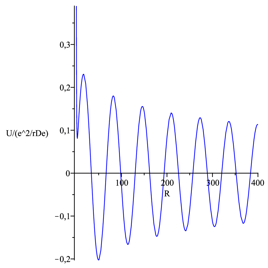
It can be clearly seen that at a long range distances the potential has an opposite sign and decays slowly as −1/r3-1/r^{3} compared to that.

Refer to caption
Figure 1: The sum of two potentials (13) and the potential (14) of two electrons in a degenerate electron-hole plasma, here R=r/rD​eR=r/r_{De}

In a general case the Eq.(8) can be deduced to the following integral

U⁡(r)=e2​rD−2​Ar3​∫0∞y2​d​y(y2​rD−2r2+1)3/2​s​i​n​(y​Ay2​rD−2r2+1)=e2​rD−2​Ar3​∫0R⋅rD−rD+y2​d​y(y2R2+1)3/2​s​i​n​(y​Ay2R2+1)=e2​rD−2r3​∫0A​r/rDz2​s​i​n​(z)​d​z(A−z2​rD−2r2)5/2\begin{gathered}U(r)=\frac{e^{2}r_{D-}^{2}\sqrt{A}}{r^{3}}\int_{0}^{\infty}\frac{y^{2}dy}{({y^{2}\frac{r_{D-}^{2}}{r^{2}}+1})^{3/2}}sin(\frac{y\sqrt{A}}{\sqrt{y^{2}\frac{r_{D-}^{2}}{r^{2}}+1}})=\frac{e^{2}r_{D-}^{2}\sqrt{A}}{r^{3}}\int_{0}^{R\cdot\frac{r_{D-}}{r_{D+}}}\frac{y^{2}dy}{({\frac{y^{2}}{R^{2}}+1})^{3/2}}sin(\frac{y\sqrt{A}}{\sqrt{\frac{y^{2}}{R^{2}}+1}})\hfill\\ =\frac{e^{2}r_{D-}^{2}}{r^{3}}\int_{0}^{\sqrt{A}r/r_{D}}\frac{z^{2}sin(z)dz}{(A-z^{2}\frac{r_{D-}^{2}}{r^{2}})^{5/2}}\end{gathered} (14)

Having solved the integral (14), we get the following from of the potential shown in Fig.1, where the integration till the k≤1/rD​ik\leq 1/r_{Di} was performed. Here, we see the multiple minima revealing the quantum nature of the phenomenon: many energy levels, see the Table 1. Here, for the existence of the energy level the following condition must be satisfied :

MIN R1R_{1} R2R_{2} Rm​i​nR_{min} U⁡(Rm​i​n)/UDU(R_{min})/U_{D} U⁡(Rm​i​n)U(R_{min}),   eV Um​i​nL{U_{min}}_{L},   eV Um​i​nL{U_{min}}_{L},   K U⁡(Rm​i​n)U(R_{min}),   K
1 33.85 66.36 50.46 -0.202 -0.053 6∗10−66*10^{-6} 0.07 622
2 98.41 130.06 114.17 -0.166 -0.044 6.47∗10−66.47*10^{-6} 0.0751 511
3 161.95 193.66 177.65 -0.147 -0.039 6.45∗10−66.45*10^{-6} 0.0749 453
4 225.35 257.12 240.88 -0.134 -0.035 6.4∗10−66.4*10^{-6} 0.0746 413
5 288.68 320.3 304.71 -0.125 -0.033 6.4∗10−66.4*10^{-6} 0.075 385
Table 1:
U⁡(Rm​i​n)>Um​i​nL=π2​ℏ24​me​a2,U(R_{min})>{U_{min}}_{L}=\frac{\pi^{2}\hbar^{2}}{4m_{e}a^{2}}, (15)

here aa - potential well width, Um​i​nL{U_{min}}_{L} - its height [3].

Let us estimate the energy levels of particles moving in a series of potential wells shown in Fig. The energy levels in a rectangular potential wells:

Em​i​nn=π2​ℏ22​me​a2n2,n=1,2⋯,N{{E_{min}}_{n}}=\frac{\pi^{2}\hbar^{2}}{2m_{e}a^{2}}n^{2},n=1,2\cdots,N (16)

where the following condition must be satisfied Um​a​x>Em​i​nnU_{m}ax>{{E_{min}}_{n}}, here S=(R2−R1)⋅Um​a​xS=(R_{2}-R_{1})\cdot U_{m}ax, SS - area of the rectangular well with the width R2−R1R_{2}-R_{1} and height Um​a​xU_{max}.
In the following Table 2 the estimated energy levels are given for a series of potential wells.

MIN R1R_{1} R2R_{2} Um​a​x,e​VU_{max},\;eV n1n_{1} Em​i​nn1,e​V{E_{min}}_{n_{1}},\;eV nNn_{N} Em​i​nnN,e​V{E_{min}}_{n_{N}},\;eV
1 33.85 66.36 -0.03235 1 −1.228⋅10−5-1.228\cdot 10^{-5} 51 −512⋅1.228⋅10−5-51^{2}\cdot 1.228\cdot 10^{-5}
2 98.41 130.06 - 0.0267 1 −1.2956⋅10−5-1.2956\cdot 10^{-5} 45 −452⋅1.2956⋅10−5-45^{2}\cdot 1.2956\cdot 10^{-5}
3 161.95 193.66 -0.0236 1 −1.29⋅10−5-1.29\cdot 10^{-5} 42 −422⋅1.29⋅10−5-42^{2}\cdot 1.29\cdot 10^{-5}
4 225.35 257.12 -0.0215 1 −1.2859⋅10−5-1.2859\cdot 10^{-5} 40 −402⋅1.2859⋅10−5-40^{2}\cdot 1.2859\cdot 10^{-5}
5 288.68 320.3 1 - 0.01997 1.298⋅10−51.298\cdot 10^{-5} 39 −392⋅1.298⋅10−5-39^{2}\cdot 1.298\cdot 10^{-5}
⋅\cdot ⋅\cdot ⋅\cdot ⋅\cdot ⋅\cdot ⋅\cdot ⋅\cdot ⋅\cdot
45 2812.6 2844.12 0.0072 1 1.306⋅10−51.306\cdot 10^{-5} 23 −232⋅1.306⋅10−5-23^{2}\cdot 1.306\cdot 10^{-5}
⋅\cdot ⋅\cdot ⋅\cdot ⋅\cdot ⋅\cdot ⋅\cdot ⋅\cdot ⋅\cdot
120 7538.75 7570.26 0.00362 1 1.307⋅10−51.307\cdot 10^{-5} 16 −162⋅1.307⋅10−5-16^{2}\cdot 1.307\cdot 10^{-5}
Table 2:

3 Discussion of the results and quantitative estimations

From the made above analysis, we can conclude that interaction between two electrons at the distances much larger than the Debye electron radius changes its sign and becomes attractive. This potential amplitude is much higher than that, repulsive one, at the short distances and can lead to the bound state of two electrons (Cooper pair).
I would like to express my deepest gratitude and appreciation to Prof. Dr. A. A. Rukhadze for such a long fruitful collaboration with me and personal support.

References

  • [1] A.F. Alexandrov, L.S. Bogdankevich, A.A. Rukhadze, Principles of Plasma Electrodynamics (Springer, Heidelberg, 1984), pp. 167-170.
  • [2] Livshits E. M., Pitaevsky L.P., Physical Kinetics (Pergamon Press, London, 1982).
  • [3] Livshits E. M., Pitaevsky L.P., Quantum Mechanics (Pergamon Press, London, 1982).