Differentiability versus continuity: Restriction and extension theorems and monstrous examples

Krzysztof C. Ciesielski Address: Department of Mathematics,
West Virginia University, Morgantown,
WV 26506-6310, USA.
and
Department of Radiology, MIPG,
University of Pennsylvania,
Philadelphia, PA 19104-6021, USA. Email address: KCies@math.wvu.edu and Juan B. Seoane–Sepúlveda Address: Instituto de Matemática Interdisciplinar (IMI),
Departamento de Análisis y Matemática Aplicada,
Facultad de Ciencias Matemáticas,
Plaza de Ciencias 3,
Universidad Complutense de Madrid,
28040 Madrid, Spain. Email address: jseoane@ucm.es

Abstract.

The aim of this expository article is to present recent developments in the centuries old discussion on the interrelations between continuous and differentiable real valued functions of one real variable. The truly new results include, among others, the $D^{n}$ - $C^{n}$ interpolation theorem: For every $n$ -times differentiable $f\colon{\real}\to{\real}$ and perfect $P\subset{\real}$ there is a $C^{n}$ function $g\colon{\real}\to{\real}$ such that $f\restriction P$ and $g\restriction P$ agree on an uncountable set and an example of a differentiable function $F\colon{\real}\to{\real}$ (which can be nowhere monotone) and of compact perfect $\mathfrak{X}\subset{\real}$ such that $F^{\prime}(x)=0$ for all $x\in\mathfrak{X}$ while $F[\mathfrak{X}]=\mathfrak{X}$ ; thus, the map $\mathfrak{f}=F\restriction\mathfrak{X}$ is shrinking at every point while, paradoxically, not globally. However, the novelty is even more prominent in the newly discovered simplified presentations of several older results, including: a new short and elementary construction of everywhere differentiable nowhere monotone $h\colon{\real}\to{\real}$ and the proofs (not involving Lebesgue measure/integration theory) of the theorems of Jarník: Every differentiable map $f\colon P\to{\real}$ , with $P\subset{\real}$ perfect, admits differentiable extension $F\colon{\real}\to{\real}$ and of Laczkovich: For every continuous $g\colon{\real}\to{\real}$ there exists a perfect $P\subset{\real}$ such that $g\restriction P$ is differentiable. The main part of this exposition, concerning continuity and first order differentiation, is presented in an narrative that answers two classical questions: To what extend a continuous function must be differentiable? and How strong is the assumption of differentiability of a continuous function? In addition, we overview the results concerning higher order differentiation. This includes the Whitney extension theorem and the higher order interpolation theorems related to Ulam-Zahorski problem. Finally, we discuss the results concerning smooth functions that are independent of the standard axioms ZFC of set theory. We close with a list of currently open problems related to this subject.

Key words and phrases:

continuous function, differentiable function, points of continuity, points of differentiability, Whitney extension theorem, interpolation theorems, independence results, classification of real functions, Baire classification functions, Pompeiu derivative

2010 Mathematics Subject Classification

26A24, 54C30, 46T20, 58B10, 54A35, 26A21, 26A27, 26A30, 54C20, 41A05

1. Introduction and overview

Continuity and Differentiability are among the most fundamental concepts of differential calculus. Students often struggle to fully comprehend these deep notions. Of course, as we all know, differentiability is a much stronger condition than continuity. Also, continuity can behave in many strange ways. For instance, besides the classical definition of continuous function, there are many characterizations of this concept that, usually, are not taught at an undergraduate level. One of these characterization (due to Hamlett [59], see also [54, 17, 114, 72, 119] for further generalizations) states that a function $f$ from to is continuous if, and only if, $f$ maps continua (compact, connected sets) to continua. On the contrary, and quite surprisingly, there are nowhere continuous functions mapping connected sets to connected sets, and (separately) compact sets to compact sets ([55]). Somehow, a key direction of study of continuity and differentiability deals with trying to provide a clear structure of what the set of points of continuity/differentiability looks like.

The leading theme of this expository paper is to discuss the following two questions concerning the functions from to :

Q1:

How much continuity does differentiability imply?
Q2:

How much differentiability does continuity imply?

They will be addressed in Sections 2 and 3, respectively. The main narrative presented in these sections is independent of any results from Lebesgue measure and/or integration theory. In particular, it can be incorporated into an introductory course of real analysis. The question Q1, addressed in Section 2, will be interpreted as a question on the continuity of the derivatives. We will recall that the derivatives must have the intermediate value property and must be continuous on a dense $G_{\delta}$ -set.¹¹ 1 As usual, we say that a set is a $G_{\delta}$ -set whenever is the countable intersection of open sets. The key novelty here will be a presentation of recently found simple construction of a differentiable monster, that is, a differentiable function that is nowhere monotone. The existence of such examples shows that none of the good properties of the derivatives discussed earlier can be improved. Towards the answer of Q2, presented in Section 3, we start with a construction of a Weierstrass monster, that is, a continuous function which is differentiable at no point. Then, we proceed to show that for every continuous functions $f\colon{\real}\to{\real}$ there exists a compact perfect set $P\subset{\real}$ such that the restriction $f\restriction P$ is differentiable. Moreover, there exists a $C^{1}$ (i.e., continuously differentiable) function $g\colon{\real}\to{\real}$ for which the set $[f=g]\coloneqq\{x\in{\real}\colon f(x)=g(x)\}$ is uncountable, the result known as $C^{1}$ -interpolation theorem. This function $g$ will be constructed using a recently found version of a Differentiable Extension Theorem of Jarník. As a part of this discussions we also show that differentiable functions from a compact perfect set $P\subset{\real}$ into can behave quite paradoxical, by describing a simple construction of a perfect subset $\mathfrak{X}$ of the Cantor ternary set ${\mathfrak{C}}\subset{\real}$ and a differentiable surjection $\mathfrak{f}\colon\mathfrak{X}\to\mathfrak{X}$ such that $\mathfrak{f}\,^{\prime}\equiv 0$ .

In Section 4 we shall discuss the extension and interpolation theorems for the classes of functions from to of higher smoothness: $D^{n}$ , of $n$ -times differentiable functions, and $C^{n}$ , of those functions from $D^{n}$ whose $n$ th derivative is continuous.

Section 5 shall provide a set theoretical flavor to this expository paper by giving an overview of the results related to smooth functions which are independent of the axiomatic set system ZFC. We shall go through interpolations theorems via consistency results, and provide some consequences of the Martin’s Axiom (MA), Continuum Hypothesis (CH), or Covering Property Axiom (CPA) on “how many” $C^{n}$ functions are needed in order to cover any $f\in D^{n}$ . Furthermore, and in the spirit of the classical Sierpiński decomposition, we will also consider when the plane can be covered by the graphs of few (i.e., fewer than continuum many) continuous/continuously differentiable functions. Other consistency results will be presented. At the end, some open questions and final remarks will be provided in Section 6.

2. Continuity from differentiability

Clearly any differentiable function $F\colon{\real}\to{\real}$ is continuous. Thus, the true question we will investigate here is:

Can we “squeeze” more continuity properties from the assumption of differentiability of $F$ ?

More specifically:

To what extent the derivative $F^{\prime}$ of $F$ must be continuous?

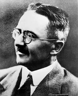
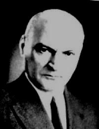
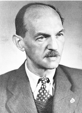
Of course, for a differentiable complex function $F\colon{\mathbb{C}}\to{\mathbb{C}}$ , its derivative is still differentiable and, thus, continuous. The same is true for any real analytic function $F(x)\coloneqq\sum_{n=0}^{\infty}a_{n}x^{n}$ . Moreover, one of the most astonishing results, due to Augustin Louis Cauchy²² 2 We include the pictures and birth-to-death years of the main contributors to this story who are already deceased. (1789-1857), [20], in the theory of complex variables states that for functions of a single complex variable, a function being analytic is equivalent to it being holomorphic. Recall that, although the term analytic function is often used interchangeably with that of holomorphic function, the word analytic is defined in a much broader sense in order to denote any function (real, complex, or of more general type) that can be written as a convergent power series in a neighborhood of each point in its domain.

Refer to caption — Figure 1. Augustin Louis Cauchy.

For the functions from to the situation is considerably more complicated. It is true that most of the derivatives we see in regular calculus courses are continuous. Nevertheless (in spite of what probably many calculus students believe) there exist differentiable functions from to with discontinuous derivatives. This is commonly exemplified by a map $h\colon{\real}\to{\real}$ given by (1), which appeared already in a 1881 paper [115, p. 335] of Vito Volterra (1860-1940):

(1)

h(x)\coloneqq\begin{cases}x^{2}\sin\left(x^{-1}\right)&\mbox{ for $x\neq 0$},\\ 0&\mbox{ for $x=0$},\\ \end{cases}

(see Fig. 2) with the derivative³³ 3 $h^{\prime}(0)=0$ follows from the squeeze theorem, since $\left|\frac{h(x)-h(0)}{x-0}\right|\leq\left|\frac{x^{2}-h(0)}{x-0}\right|=|x|$ .

h^{\prime}(x)\coloneqq\begin{cases}2x\sin\left(x^{-1}\right)-\cos\left(x^{-1}\right)&\mbox{ for $x\neq 0$},\\ 0&\mbox{ for $x=0$}.\\ \end{cases}

The existence of such examples lead mathematicians to the investigation of which functions are the derivatives and, more generally, of the properties that the derivatives must have. The systematic study of the structure of derivatives (of functions from to ) can be traced back to at least the second half of the 19th century. The full account of these studies can be found in the 250 page monograph [13] of Andrew Michael Bruckner (1932–) from 1978 (with bibliography containing 218 items) and its 1994 updated edition [15]. The limited scope of this article does not allow us to give a full account of such a vast material. Instead, we will focus here on the results that are best suited to this narrative.

We will start with discussing the “nice” properties of the class of derivatives, that is, those that coincide with the properties of the class of all continuous functions.

2.1. Nice properties of derivatives

Of course, by the Fundamental Theorem of Calculus, any continuous function $f\colon{\real}\to{\real}$ is a derivative of $F\colon{\real}\to{\real}$ defined as $F(x)\coloneqq\int_{0}^{x}f(t)\;dt$ . Also, in spite of the existence of discontinuous derivatives, the derivatives share several ‘‘good” properties of continuous functions. For example, the derivatives form a vector space:⁴⁴ 4 However, the product of a two derivatives need not be a derivative. For example, if $F(x)\coloneqq x^{2}\sin\left(1/x^{2}\right)$ for $x\neq 0$ and $F(0)\coloneqq 0$ , then $F$ is differentiable, but $(F^{\prime})^{2}$ is not a derivative (see, e.g., [13, page 17]). this follows from a basic differentiation formula, that $(a\,f(x)+b\,g(x))^{\prime}=a\,f^{\prime}(x)+b\,g^{\prime}(x)$ for every differentiable functions $f,g\colon{\real}\to{\real}$ . Also, similarly as any continuous function, any derivative has the intermediate value property, as shown by Jean-Gaston Darboux (1842-1917) in his 1875 paper [41].

Theorem 2.1.

Any derivative $f\colon{\real}\to{\real}$ has the intermediate value property, that is, for every $a<b$ and $y$ between $f(a)$ and $f(b)$ there exists an $x\in[a,b]$ with $f(x)=y$ .

Proof.

Assume that $f(a)\leq y\leq f(b)$ (the case $f(b)\leq y\leq f(a)$ is similar). Let $F\colon{\real}\to{\real}$ be such that $F^{\prime}=f$ and define $\varphi\colon{\real}\to{\real}$ as $\varphi(t)\coloneqq F(t)-yt$ . Then $\varphi^{\prime}(t)=f(t)-y$ and $\varphi^{\prime}(a)=f(a)-y\leq 0\leq f(b)-y=\varphi^{\prime}(b)$ . We need to find an $x\in[a,b]$ with $\varphi^{\prime}(x)=0$ . This is obvious, unless $\varphi^{\prime}(a)<0<\varphi^{\prime}(b)$ , in which case the maximum value of $\varphi$ on $[a,b]$ , existing by the extreme value theorem, must be attained at some $x\in(a,b)$ . For such $x$ we have $\varphi^{\prime}(x)=0$ .

An alternative proof of Theorem 2.1 can be found in [96]. Because of Darboux’s work, nowadays the functions from to that have the intermediate value property (or, more generally, the functions from a topological space $X$ into a topological space $Y$ that map connected subsets of $X$ onto connected subsets of $Y$ ) are often called Darboux functions.

It is easy to see that a composition of Darboux functions remains Darboux. Thus, the composition of derivatives, similarly as the composition of continuous functions on , still enjoys the intermediate value property, in spite the fact that a composition of two derivatives need not be a derivative.⁵⁵ 5 For example, if $F$ is as in the footnote 4, then $(F^{\prime})^{2}$ is a composition of two derivatives, $F^{\prime}(x)$ and $g(x)\coloneqq x^{2}$ , which is not a derivative.

The next result, that comes from the 1899 dissertation [5] of René-Louis Baire (1874-1932), shows that every derivative must have a lot of points of continuity. (See also [88].) This research of Baire is closely related to another fascinating real analysis topic: the study of separately continuous functions (i.e., of functions $g\colon{}^{2}\to{\real}$ for which the sectional maps $g(x,\cdot)$ and $g(\cdot,x)$ are continuous for all $x\in{\real}$ ),⁶⁶ 6 It is easy to see that $f\colon{\real}\to{\real}$ is differentiable if, and only if, the difference quotient map $q(x,y)\coloneqq\frac{f(x)-f(y)}{x-y}$ , defined for all $x\neq y$ , can be extended to a separately continuous map $g\colon{}^{2}\to{\real}$ , with $g(x,x)=f^{\prime}(x)$ for all $x\in{\real}$ . In this context, we sometimes refer to the functions of more than one variable as jointly continuous if they are continuous in the usual (topological) sense. recently surveyed by the first author and David Alan Miller [28]. (Most interestingly, Cauchy, in his 1821 book Cours d’analyse [21], proves that separate continuity implies continuity, which is well known to be false. Nevertheless, as explained in [28], Cauchy was not mistaken!)

Theorem 2.2.

The derivative of any differentiable function $F\colon{\real}\to{\real}$ is Baire class one, that is, it is a pointwise limit of continuous functions. In particular, since the set of points of continuity of any Baire class one function is a dense $G_{\delta}$ -set, the same is true for $F^{\prime}$ .

Proof.

Clearly $F^{\prime}$ is a pointwise limit of continuous functions, since we have $F^{\prime}(x)=\lim_{n\to\infty}F_{n}(x)$ , where functions $F_{n}(x)\coloneqq\frac{f(x+1/n)-f(x)}{1/n}$ are clearly continuous.

Also, for any function $g\colon{\real}\to{\real}$ , the set $C_{g}$ of points of continuity of $g$ is a $G_{\delta}$ -set: $C_{g}\coloneqq\bigcap_{n=1}^{\infty}V_{n}$ , where the sets

V_{n}\coloneqq\bigcup_{\delta>0}\{x\in{\real}\colon\mbox{$|g(s)-f(g)|<1/n$ for all $s,t\in(x-\delta,x+\delta)$}\}

are open. At the same time, any pointwise limit $g\colon{\real}\to{\real}$ of continuous functions $g_{n}\colon{\real}\to{\real}$ is continuous on a dense $G_{\delta}$ -set $G\coloneqq\bigcap_{n=1}^{\infty}\bigcup_{N=1}^{\infty}U^{n}_{N}$ , where each $U^{n}_{N}$ is the interior of the closed set

\{x\in{\real}\colon|f_{k}(x)-f_{m}(x)|\leq 1/n\mbox{ for all $m,k\geq N$}\}.

(See e.g., [93, theorem 48.5].) Thus, the set of points of continuity of any Baire class one function must be dense (containing a set in form of $G$ ) and a $G_{\delta}$ -set.

Another interesting property of continuous functions that is shared by derivatives is the fixed point property:

Proposition 2.3.

If $f\colon[-1,1]\to[-1,1]$ is a derivative, then it has a fixed point, that is, there exists an $x\in[-1,1]$ such that $f(x)=x$ .

Proof.

The function $g\colon[-1,1]\to{\real}$ , defined as $g(x)\coloneqq f(x)-x$ is a derivative. Thus, by Theorem 2.1, it has the intermediate value property. Since $g(-1)=f(x)+1\geq 0$ and $g(1)=f(1)-1\leq 0$ , there exists $z\in[-1,1]$ such that $f(z)-z=g(z)=0$ . Thus, $f(z)=z$ , as needed.

More interestingly, a composition of finitely many derivatives, from $[0,1]$ to $[0,1]$ , also possesses the fixed point property. For the composition of two derivatives this has been proved, independently, in [40] and [45], while the general case is shown in [107]. This happens, in spite the fact that a composition of two derivatives need not be of Baire class one (so, by Theorem 2.2, a derivative). This is shown by the following example, which is a variant of one from [11].⁷⁷ 7 The fixed point property of the composition of derivatives could be easily deduced, if it could be shown that the composition of the derivatives has a connected graph. However, it remains unknown if such a result is true, see e.g., [11] and Problem 6.2.

Example 2.4.

There exist derivatives $\varphi,\gamma\colon[-1,1]\to[-1,1]$ such that their composition $\psi\coloneqq\varphi\circ\gamma$ is not of Baire class one.

Proof.

Let $\gamma(x)\coloneqq\cos(x^{-1})$ for $x\neq 0$ and $\gamma(0)\coloneqq 0$ . It is a derivative, as a sum of two derivatives: a continuous function $f(x)\coloneqq x\sin\left(x^{-1}\right)$ for $x\neq 0$ , $f(0)\coloneqq 0$ , and function $-h^{\prime}$ , where $h$ is as in (1). The graph of $\gamma$ is of the form from the right hand side of Figure 2.

Let $\varphi(x)\coloneqq m\ h^{\prime}(x-b)$ for $x\in[-1,1]$ , where $h$ is an inverse of Pompeiu’s function from Proposition 2.8, $b\in{\real}$ is such that $h^{\prime}(b)=0$ , and $m>0$ is such that $\varphi[-1,1]\subset[-1,1]$ . Clearly, $\varphi$ is also a derivative.

To see that $\psi=\varphi\circ\gamma$ is not of Baire class one, by Theorem 2.2 it is enough to show that it is discontinuous on the set $G\coloneqq\{x\in(-1,1)\colon\varphi(x)=0\}$ , which is a dense $G_{\delta}$ . Thus, fix $x\in G$ and note that $\psi(x)=0$ . It suffices to show that, for every ${\varepsilon}>0$ such that $(x-{\varepsilon},x+{\varepsilon})\subset(-1,1)$ , there exists $y\in(x-{\varepsilon},x+{\varepsilon})$ with $\psi(y)=1$ . Indeed, since $\varphi$ is nowhere constant, there exists $z\in(x,x+{\varepsilon})$ such that $\varphi(z)>0$ . Then, since $\gamma[(0,\varphi(z))]=[-1,1]$ , there exists $p\in(0,\varphi(z)]$ such that $\gamma(p)=1$ . Also, since $\varphi$ is Darboux and $p\in(0,\varphi(z)]=(\varphi(x),\varphi(z)]$ , there exists $y\in(x,z)\subset(x,x+{\varepsilon})$ such that $\varphi(y)=p$ . Thus, $\psi(y)=\varphi(\gamma(y))=\varphi(p)=1$ , as needed.

Next we turn our attention to show, by means of illuminating examples, that the nice properties of the derivatives we stated above cannot be improved in any essential way.

2.2. Differentiable monster and other examples

We start here with showing that all that can be said about the set of points of continuity of derivatives is already stated in Theorem 2.2.

Theorem 2.5.

For every dense $G_{\delta}$ -set $G\subset{\real}$ there exists a differentiable function $f\colon{\real}\to{\real}$ such that $G$ is the set of points of continuity of the derivative $f^{\prime}$ .

Sketch of proof.

Choose $d\in(0,1)$ such that $h^{\prime}(d)=0$ , where $h$ is as in (1). For every closed nowhere dense $E\subset{\real}$ define $f_{E}\colon{\real}\to[-1,1]$ via

f_{E}(x)\coloneqq\begin{cases}\displaystyle h\left(\frac{2d\,{\rm dist}(x,\{a,b\})}{b-a}\right)&\mbox{ for $x$ in a component $(a,b)$ of ${\real}\setminus E$,}\\ 0&\mbox{ for $x\in E$}.\end{cases}

This is a variant of a Volterra function from [115]. It is easy to see that $f_{E}$ is differentiable with the derivative continuous on ${\real}\setminus E$ and having oscillation 2 at every $x\in E$ .

Now, if $G\subset{\real}$ is a dense $G_{\delta}$ , then $\real\setminus G\coloneqq\bigcup_{n<\omega}E_{n}$ , some some family $\{E_{n}\colon n<\omega\}$ of closed nowhere dense sets in . In particular (see e.g. [103, Theorem 7.17]), the function $f\coloneqq\sum_{n<\omega}3^{-n}f_{E_{n}}$ is differentiable and its derivative $f^{\prime}=\sum_{n<\omega}3^{-n}f_{E_{n}}^{\prime}$ is continuous precisely at the points of $G$ .

Theorems 2.2 and 2.5 immediately give the following characterization of the sets of points of continuity of the derivatives.

Corollary 2.6.

For a $G\subset{\real}$ , there exists a differentiable function $f\colon{\real}\to{\real}$ such that $G$ is the set of points of continuity of its derivative $f^{\prime}$ if, and only if, $G$ is a dense $G_{\delta}$ -set.

Next, we will turn our attention to an example of a differentiable function which is one of the strangest, most mind-boggling examples in analysis.

2.2.1. Differentiable nowhere monotone maps

We will start with the following elementary example showing that, for a differentiable function $\psi\colon{\real}\to{\real}$ , a non-zero value of the derivative at a point does not imply the monotonicity of the function in a neighborhood of the point. For instance (see [57]), this is the case for $\psi(x)\coloneqq x+2h(x)$ , where $h$ is given by (1), that is,

\psi(x)\coloneqq\begin{cases}x+2x^{2}\sin(x^{-1})&\mbox{ for $x\neq 0$,}\\ 0&\mbox{ for $x=0$,}\\ \end{cases}

see Fig. 5. Indeed $\psi^{\prime}(0)=1$ , while $\psi$ is not monotone on any non-empty interval $(-\delta,\delta)$ .

Figure 5. The graphs of

\psi

and

\psi^{\prime}

The example from the next theorem pushes this pathology to the extreme.

Theorem 2.7.

There exists a differentiable function $f\colon{\real}\to{\real}$ which is monotone on no non-trivial interval. In particular, each of the sets

Z_{f}\coloneqq\{x\in{\real}\colon f^{\prime}(x)=0\}\text{ and }Z_{f}^{c}\coloneqq\{x\in{\real}\colon f^{\prime}(x)\neq 0\}

is dense and $f^{\prime}$ is discontinuous at every $x\in Z_{f}^{c}$ .

The graph of such a function is simultaneously smooth and very rugged. This sounds (at least to us) like an oxymoron. Therefore, we started to refer to such functions as differentiable monsters, see [36]. Of course, a differentiable monster $f$ must attain local maximum (as well as local minimum) on every interval. In particular, the set $Z_{f}$ must indeed be dense. Its complement, $Z_{f}^{c}$ , must also be dense, since otherwise $f$ would be constant on some interval.

The history of differentiable monsters is described in detail in the 1983 paper of A. M. Bruckner [14]. The first construction of such a function was given in 1887 (see [77]) by Alfred Köpcke (1852-1932). (There was, originally, a gap in [77], but it was subsequently corrected in [78, 79].) The most influential study of this subject is a 1915 paper [42] of Arnaud Denjoy (1884–1974). The construction we describe below comes from a recent paper [36] of the first author. It is simpler than the constructions from the 1974 paper [68] of Yitzhak Katznelson (1934–) and Karl Stromberg (1931–1994) and from the 1976 article [118] of Clifford Weil. There are quite a few different technical constructions of such monster, some of them including (for instance) the use of wavelets (see the work by R.M. Aron, V.I. Gurariy and the second author, [2] or, also, [53]).

As a matter of fact (and with the appropriate background) our construction of a differentiable monster can be reduced to a single line:

f(x)\coloneqq h(x-t)-h(x)

, where

h

is the inverse of a Pompeiu’s map

g

as described below and $t$ is an arbitrary number from some residual set (i.e., a set containing a dense $G_{\delta}$ -set). A more detailed argument follows.

Pompeiu’s functions.

Let $Q\coloneqq\{q_{i}\colon i\in{\mathbb{N}}\}$ be an enumeration of a countable dense subset of (e.g., the set ${{\mathbb{Q}}}$ of rational numbers) such that $|q_{i}|\leq i$ for all $i\in{\mathbb{N}}$ . Fix an $r\in(0,1)$ and let $g\colon{\real}\to{\real}$ be defined by $g(x)\coloneqq\sum_{i=1}^{\infty}r^{i}(x-q_{i})^{1/3}.$ This $g$ is essentially⁸⁸ 8 Usually $g$ is defined on $[0,1]$ as $\hat{g}(x)\coloneqq\sum_{i=1}^{\infty}a_{i}(x-q_{i})^{1/3}$ , where $Q$ is an arbitrary enumeration of ${{\mathbb{Q}}}\cap[0,1]$ and numbers $a_{i}>0$ are arbitrary so that $\sum_{i=1}^{\infty}a_{i}$ converges. This $\hat{g}$ can also be transformed into the function $g\colon{\real}\to{\real}$ we need, rather than using our definition. Specifically, if $[c,d]=\hat{g}[[0,1]]$ , then we can take $g\coloneqq h_{1}\circ\hat{g}\circ h_{0}$ , where $h_{0}$ and $h_{1}$ are the diffeomorphisms from onto $(0,1)$ and from $(c,d)$ onto , respectively. the function constructed in the 1907 paper [100] of Dimitrie Pompeiu (1873–1954), as seen in Fig. 7. (See [36]. Compare also [14] or [111, section 9.7].)

Intuitively, $g$ has a non-horizontal tangent line at every point, vertical at each $(q_{i},g(q_{i}))$ , since the same is true for the map $(x-q_{i})^{1/3}$ . The graph of its inverse, $h$ , is the reflection of the graph of $g$ with respect to the line $y=x$ . So, $h$ also has a tangent line at every point, the vertical tangent lines of $g$ becoming horizontal tangents of $h$ .

Figure 7. Rough sketch of the graph of a partial sum of Pompeiu’s original example, function

g

and its derivative, constructed over the interval

[0,1]

More formally,

Proposition 2.8.

The map $g$ is continuous, strictly increasing, and onto . Its inverse $h\coloneqq g^{-1}\colon{\real}\to{\real}$ is everywhere differentiable with $h^{\prime}\geq 0$ and such that the sets $Z\coloneqq\{x\in{\real}\colon h^{\prime}(x)=0\}$ and $Z^{c}\coloneqq\{x\in{\real}\colon h^{\prime}(x)\neq 0\}$ are both dense in .

Proof.

The series

g(x)\coloneqq\sum_{i=1}^{\infty}r^{i}(x-q_{i})^{1/3}

converges uniformly on every bounded set:

|g(x)|\leq\sum_{i=1}^{\infty}r^{i}(|x|+i+1)

since

\left|(x-q_{i})^{1/3}\right|\leq(|x|+|q_{i}|+1)^{1/3}\leq|x|+|q_{i}|+1\leq|x|+i+1.

Thus, $g$ is continuous. It is strictly increasing and onto , since that is true of every term $\psi_{i}(x)\coloneqq r^{i}(x-q_{i})^{1/3}$ .

The trickiest part is to show that

(2)

g^{\prime}(x)=\sum_{i=1}^{\infty}\psi_{i}^{\prime}(x)\left(=\sum_{i=1}^{\infty}r^{i}\frac{1}{3}\frac{1}{(x-q_{i})^{2/3}}\right).

However, this clearly holds when $\sum_{i=1}^{\infty}\psi_{i}^{\prime}(x)=\infty$ , since then, for every $y\neq x$ , we have

\frac{g(x)-g(y)}{x-y}=\sum_{i=1}^{\infty}\frac{\psi_{i}(x)-\psi_{i}(y)}{x-y}\geq\sum_{i=1}^{n}\frac{\psi_{i}(x)-\psi_{i}(y)}{x-y},

and the last expression is arbitrarily large for large enough $n$ and $y$ close enough to $x$ . On the other hand, when $\sum_{i=1}^{\infty}\psi_{i}^{\prime}(x)<\infty$ , then (2) follows from the fact that

0<\frac{\psi_{i}(x)-\psi_{i}(y)}{x-y}\leq 6\psi_{i}^{\prime}(x)

for every $y\neq x$ .⁹⁹ 9 It is enough to prove this for $\psi(x)\coloneqq x^{1/3}$ . It holds for $x=0$ , as $\psi^{\prime}(0)=\infty$ . Also, since $\psi(x)$ is odd and concave on $(0,\infty)$ , we can assume that $x>0$ and $y<x$ . Then $L(y)<\psi(y)$ , where $L$ is the line passing through $(x,\psi(x))$ and $(0,-\psi(x))$ . So, $0<\frac{\psi(x)-\psi(y)}{x-y}<\frac{L(x)-L(y)}{x-y}=\frac{2x^{1/3}}{x}=6\psi^{\prime}(x)$ , as needed. Indeed, given ${\varepsilon}>0$ and $n\in{\mathbb{N}}$ for which $\sum_{i=n+1}^{\infty}\psi_{i}^{\prime}(x)<{\varepsilon}/14$ ,

	$\displaystyle\left\|\frac{g(x)-g(y)}{x-y}-\sum_{i=1}^{\infty}\psi_{i}^{\prime}(x)\right\|$	$\displaystyle\leq\sum_{i=1}^{n}\left\|\frac{\psi_{i}(x)-\psi_{i}(y)}{x-y}-\psi_{i}^{\prime}(x)\right\|+7\left\|\sum_{i=n+1}^{\infty}\psi_{i}^{\prime}(x)\right\|$
		$\displaystyle\leq\sum_{i=1}^{n}\left\|\frac{\psi_{i}(x)-\psi_{i}(y)}{x-y}-\psi_{i}^{\prime}(x)\right\|+\frac{{\varepsilon}}{2}$

which is less than ${\varepsilon}$ for $y$ close enough to $x$ .

Now, by (2), $g^{\prime}(x)=\infty$ on the dense set $Q$ . Therefore, the inverse $h\coloneqq g^{-1}$ is strictly increasing and differentiable, with $h^{\prime}\geq 0$ . The set $Z\coloneqq\{x\in{\real}\colon h^{\prime}(x)=0\}$ is dense in , since it contains the dense set $g[Q]$ . The complement of $Z$ must be dense since, otherwise, $h$ would be constant on some interval.

Construction of $f$ from Theorem 2.7.

Let $h$ , $Z$ , and $Z^{c}$ be as in Proposition 2.8 and let $D\subset{\real}\setminus Z$ be countable and dense. Since $h^{\prime}$ is discontinuous at every $x\in Z^{c}$ , we conclude from Theorem 2.2 that the set $G\coloneqq\bigcap_{d\in D}\bigl((-d+Z)\cap(d-Z)\bigr)$ is residual. We claim that, for any $t\in G$ , the function $f\colon{\real}\to{\real}$ defined as $f(x)\coloneqq h(x-t)-h(x)$ is a differentiable monster.

Indeed, clearly $f$ is differentiable with $f^{\prime}(x)=h^{\prime}(x-t)-h^{\prime}(x)$ . Also, $f^{\prime}>0$ on $t+D$ , since for every $d\in D$ we have $t+d\in Z$ , so that

f^{\prime}(t+d)=h^{\prime}(d)-h^{\prime}(t+d)=h^{\prime}(d)>0.

Similarly, $f^{\prime}<0$ on $D$ , since for every $d\in D$ we have $d-t\in Z$ , so that $f^{\prime}(d)=h^{\prime}(d-t)-h^{\prime}(d)=-h^{\prime}(d)<0$ .

2.2.2. More examples related to calculus

One of the first things we learn in calculus is that if for a differentiable function $\varphi\colon{\real}\to{\real}$ its derivative changes sign at a point $p$ , then $\varphi$ has a (local) proper extreme value at $p$ .

Our fist example here (see also [57]) shows that the change of sign of the derivative is not necessary for the existence of a proper extreme value at $p$ . For instance, this is the case for $\varphi(x)\coloneqq 2x^{4}+x^{2}h(x)$ , where $h$ is given by (1), that is,

\varphi(x)\coloneqq\begin{cases}x^{4}\left(2+\sin(x^{-1})\right)&\mbox{ for $x\neq 0$,}\\ 0&\mbox{ for $x=0$,}\\ \end{cases}

see Fig. 8. It is easy to see that it has a proper minimum at $p=0$ , while its derivative does no change sign at $0$ .

Figure 8. The graphs of

\varphi

and

\varphi^{\prime}

The second example here (see also [57]) shows that a derivative of a differentiable function $\eta\colon{\real}\to{\real}$ need not satisfy the Extrema Value Theorem (even though it satisfies the Intermediate Value Theorem). For instance, this is the case for $\eta(x)\coloneqq e^{-3x}h(x)$ , where $h$ is given by (1), that is,

\eta(x)\coloneqq\begin{cases}e^{-3x}x^{2}\sin(x^{-1})&\mbox{ for $x\neq 0$,}\\ 0&\mbox{ for $x=0$,}\\ \end{cases}

see Fig. 9.

The Extrema Value Theorem fails for $\eta^{\prime}$ , since $\inf\eta^{\prime}[[0,1/3]]=-1\notin\eta^{\prime}[[0,1/3]]$ . To see this, note that $\eta^{\prime}(x)=-3e^{-3x}h(x)+e^{-3x}h^{\prime}(x)$ , that is, $\eta^{\prime}(0)=0$ and

\eta^{\prime}(x)=e^{-3x}\left(-3x^{2}\sin(x^{-1})+2x\sin(x^{-1})-\cos(x^{-1})\right)

for $x\neq 0.$

In particular, on $(0,1/3]$ , we have

|\eta^{\prime}(x)|\leq e^{-3x}\left(3x^{2}+2x+1\right)\leq e^{-3x}\left(1+3x\right)<1,

where the last inequality holds since, by Taylor formula,

e^{3x}=\sum_{i=0}^{\infty}\frac{(3x)^{i}}{i!}>1+3x.

This justify $-1\notin\eta^{\prime}([0,1/3])$ . As the same time, for $x_{n}\coloneqq(2\pi n)^{-1}$ , we have $\lim_{n\to\infty}\eta^{\prime}(x_{n})=\lim_{n\to\infty}-e^{-x_{n}^{2}}=-1$ , that is, indeed $\inf\eta^{\prime}([0,1/3])=-1$ .

Figure 9. Graphs of

\eta

and

\eta^{\prime}

This last example, $\eta$ , can be pushed even further, as shown by A. W. Bruckner in [13, §VI, Theorem 3.1]: there are derivatives defined on a closed interval that achieve no local extrema (i.e., maximum or minimum). However, their constructions is considerably more complicated. Many more pathologies of this kind can be found in the excellent monograph [57]. See also [6, 57, 39, 3, 46, 19, 71, 69] for a long list of pathologies enjoyed by continuous and differentiable functions in $\mathbb{R}^{\mathbb{R}}$ .

It is appropriate to finish this section recalling that there is no characterization of the derivatives simpler than the trivial one:

$f$ is a derivative if, and only if, there exists an $F$ for which $f=F^{\prime}$ .

Perhaps, a simpler characterization can never be found. (See, e.g., [51].)

3. Differentiability from continuity

In this section we will address the question

Q2: How much differentiability does continuity imply?

We will argue, in spite of what the next example shows, that actually every continuous function has some traces of differentiability.

3.1. Weierstrass monsters

At a first glance, an answer to the question Q2 should be none, since there exist continuous functions $f\colon{\real}\to{\real}$ that are differentiable at no point $x\in{\real}$ .

Although the first known example of this kind dates back to Bernard Bolzano (1781-1848) in 1822 (see, e.g., [63]), the first published example of such an $f$ appeared in 1886 paper [116] (for the English translation see [117]) by Karl Weierstrass (1815–1897). The example, defined as

W(x)\coloneqq\sum^{\infty}_{n=0}\frac{1}{2^{n}}\cos(13^{n}\pi x),

was first presented by Weierstrass to Prussian Academy of Sciences in 1872. At that time, mathematicians commonly believed that a continuous function must have a derivative at a “significant” set of points. Thus, the example came as a general shock to the audience and was received with such disbelief that continuous nowhere differentiable functions became known as Weierstrass’s monsters.

A large number of simple constructions of Weierstrass’s monsters have appeared in the literature; see, for example, [62, 66, 110]. Our favorite is the following variant of a 1930 example of Bartel Leendert van der Waerden (1903–1996) [113] (compare [103, Thm. 7.18]), described already in a 1903 paper [108] of Teiji Takagi (1875–1960), since the proof of its properties requires only the standard tools of one-variable calculus: $f(x)\coloneqq\sum_{n=0}^{\infty}4^{n}f_{n}(x)$ , where $f_{n}(x)\coloneqq\min_{k\in{\mathbb{Z}}}\left|x-\frac{k}{8^{n}}\right|$ is the distance from $x\in{\real}$ to the set $\frac{1}{8^{n}}{\mathbb{Z}}=\{\frac{k}{8^{n}}\colon k\in{\mathbb{Z}}\}$ . (See Fig. 11.) It is continuous at each $x\in{\real}$ , since

|f(y)-f(x)|\leq\left|\sum_{i=0}^{n}4^{i}f_{i}(y)-\sum_{i=0}^{n}4^{i}f_{i}(x)\right|+\frac{1}{2^{n}}

for every $y\in{\real}$ and $n\in{\mathbb{N}}$ . It is not differentiable at any $x\in{\real}$ , since for every $n\in{\mathbb{N}}$ and $k\in{\mathbb{Z}}$ with $x\in\left[\frac{k}{8^{n}},\frac{k+1}{8^{n}}\right]$ there exists a $y_{n}\in\left\{\frac{k}{8^{n}},\frac{k+1}{8^{n}}\right\}\setminus\{x\}$ such that

	$\displaystyle\left\|\frac{f(x)-f(y_{n})}{x-y_{n}}\right\|$	$\displaystyle\geq\left\|\frac{f(\frac{k+1}{8^{n}})-f(\frac{k}{8^{n}})}{\frac{k+1}{8^{n}}-\frac{k}{8^{n}}}\right\|$
		$\displaystyle=8^{n}\left\|\sum_{i=0}^{n}4^{i}f_{i}(\frac{k+1}{8^{n}})-\sum_{i=0}^{n}4^{i}f_{i}(\frac{k}{8^{n}})\right\|\geq\frac{2}{3}4^{n-1}.$

Remark 3.1.

In fact, any typical continuous function¹⁰¹⁰ 10 Term typical is used the Baire category sense, that is, it holds for every map from a co-meager set $G\subset C([a,b])$ of functions. is a Weierstrass monster, see e.g. [93]. Actually, a typical continuous function agrees with continuum many constant functions on perfect sets. Also, in [12], the authors studied the structure of the sets in which the graphs of a residual set of continuous functions intersect with different straight lines. They showed that any typical continuous functions $f$ has a certain structure with respect to intersections with straight lines. In particular, all but at most two of the constant functions that agree anywhere with $f$ , agree on uncountable sets (and the same also holds with lines in all non-vertical directions).

3.2. Lipschitz and differentiable restrictions

The goal of this section is to prove the following 1984 theorem of Miklós Laczkovich (1948–) from [81].

Theorem 3.2.

For every continuous $f\colon{\real}\to{\real}$ there is a perfect set $Q\subset{\real}$ such that $f\restriction Q$ is differentiable.

In the statement of the theorem, the differentiability of $h\coloneqq f\restriction Q$ is understood as existence of its derivative: the function $h^{\prime}\colon Q\to\real$ where

h^{\prime}(p)\coloneqq\lim_{x\to p,\ x\in Q}\frac{h(x)-h(p)}{x-p}

for every $p\in Q$ . The proof of this theorem presented below comes from [35]. Its advantage over the original proof is that none of its steps require the tools of Lebesgue measure/integration theory.

Before we turn our attention to the proof, we like to make two remarks, which lay outside of the main narrative here (as they use Lebesgue measure tools), but give a better perspective on Theorem 3.2. The first one is a more general version of the theorem, in the form presented in the original paper [81].

Remark 3.3.

For every $E\subset{\real}$ of positive Lebesgue measure and every continuous function $f\colon E\to{\real}$ there exists a perfect $Q\subset E$ such that $f\restriction Q$ is differentiable.

It is worth to note, that the proof we present below can be easily adapted to deduce also the statement from Remark 3.3.

The next remark shows that, in general, we cannot expect that the set $Q$ in Theorem 3.2 can be either of positive Lebesgue measure or of second category.

Remark 3.4.

There exists a continuous function $f\colon{\real}\to{\real}$ such that $f\restriction Q$ can be differentiable only when $Q$ is both first category and of Lebesgue measure 0.

A function $f\colon[0,1]\to{\real}$ with such property can be chosen as one of the coordinates of the classical Peano curve that maps continuously $[0,1]$ onto $[0,1]^{2}$ . Indeed, such coordinates are nowhere approximately and $\mathcal{I}$ -approximately differentiable, as proved in 1989 by the first author, Lee Larson, and Krzysztof Ostaszewski [26]. (See also [27, example 1.4.5].) Clearly, such $f$ cannot have a differentiable restriction to a set $Q$ of positive measure (second category) since then $f$ would be approximately ( $\mathcal{I}$ -approximately) differentiable at any density ( $\mathcal{I}$ -density) point of $Q$ .

The main tool in the presented proof of Theorem 3.2 is the following result, which is of independent interest. Notice that Theorem 3.5 follows also easily from the interpolation Theorem 3.10, whose original proof was not using Theorem 3.5.¹¹¹¹ 11 If $g\colon{\real}\to{\real}$ is a $C^{1}$ function from Theorem 3.10, then, by the Mean Value Theorem, its restriction $g\restriction[-M,M]$ is Lipschitz for every $M>0$ . Thus, for some $M>0$ , the set $P\coloneqq[f=g]\cap[-M,M]$ is perfect non-empty and $f\restriction P=g\restriction P$ is Lipschitz. However, our proof of Theorem 3.10 uses Theorem 3.5.

Theorem 3.5.

Assume that $f\colon{\real}\to{\real}$ is monotone and continuous on a non-trivial interval $[a,b]$ . For every $L>\left|\frac{f(b)-f(a)}{b-a}\right|$ there exists a closed uncountable set $P\subset[a,b]$ such that $f\restriction P$ is Lipschitz with constant $L$ .

The difficulty in proving Theorem 3.5 without measure theoretical tools comes from the fact that there exist functions like Pompeiu map from Proposition 2.8: strictly increasing continuous maps $f\colon{\real}\to{\real}$ which posses finite or infinite derivative at every point, but such that the derivative of $f$ is infinite on a dense $G_{\delta}$ -set. These examples show that a perfect set in Theorem 3.5 should be nowhere sense. Thus, we will use a measure theoretical approach, in which the measure theoretical tools will be present only implicitly or, as in case of Fact 3.7, given together with a simple proof.

The presented proof of Theorem 3.5 is extracted from a proof of a Lebesgue theorem that every monotone function $f\colon{\real}\to{\real}$ is differentiable almost everywhere. It is based on the following 1932 result of Frigyes Riesz (1880-1956) from [101], known as the rising sun lemma, see Fig. 14. See also [109].

Lemma 3.6.

If $g$ is a continuous function from a non-trivial interval $[a,b]$ into , then the set $U\coloneqq\{x\in[a,b)\colon g(x)<g(y)\mbox{ for some }y\in(x,b]\}$ is open in $[a,b)$ and $g(c)\leq g(d)$ for every connected component $(c,d)$ of $U$ .

Proof.

It is clear that $U$ is open in $[a,b)$ . To see the other part, let $(c,d)$ be a component of $U$ . By continuity of $g$ , it is enough to prove that $g(p)\leq g(d)$ for every $p\in(c,d)$ . Assume by way of contradiction that $g(d)<g(p)$ for some $p\in(c,d)$ and let $x\in[p,b]$ be a point at which $g\restriction[p,b]$ achieves the maximum. Then $g(d)<g(p)\leq g(x)$ and so we must have $x\in[p,d)\subset U$ , as otherwise $d$ would belong to $U$ . But $x\in U$ contradicts the fact that $g(x)\geq g(y)$ for every $y\in(x,b]$ .

For an interval $I$ let $\ell(I)$ be its length. We need the following simple well-known observations.

Fact 3.7.

Let $a<b$ and ${\mathcal{J}}$ be a family of open intervals with $\bigcup{\mathcal{J}}\subset(a,b)$ .

(i)

If $[\alpha,\beta]\subset\bigcup{\mathcal{J}}$ , then $\sum_{I\in{\mathcal{J}}}\ell(I)>\beta-\alpha$ .
(ii)

If the intervals in ${\mathcal{J}}$ are pairwise disjoint, then $\sum_{I\in{\mathcal{J}}}\ell(I)\leq b-a$ .

Proof.

(i): By compactness of $[\alpha,\beta]$ we can assume that ${\mathcal{J}}$ is finite, say of size $n$ . Then (i) follows by an easy induction on $n$ : if $(c,d)=J\in{\mathcal{J}}$ contains $\beta$ , then either $c\leq\alpha$ , in which case (i) is obvious, or $\alpha<c$ and, by induction, $\sum_{I\in{\mathcal{J}}}\ell(I)=\ell(J)+\sum_{I\in{\mathcal{J}}\setminus\{J\}}\ell(I)>\ell([c,\beta])+\ell([\alpha,c])=\beta-\alpha$ .

(ii): Once again, it is enough to show (ii) for finite ${\mathcal{J}}$ , say of size $n$ , by induction. Then, there is $(c,d)=J\in{\mathcal{J}}$ to the right of any $I\in{\mathcal{J}}\setminus\{J\}$ . So, by induction, $\sum_{I\in{\mathcal{J}}}\ell(I)=\ell(J)+\sum_{I\in{\mathcal{J}}\setminus\{J\}}\ell(I)\leq(b-c)+(c-a)=b-a$ .

Proof of Theorem 3.5.

If there exists a nontrivial interval $[c,d]\subset[a,b]$ on which $f$ is constant, then clearly $P\coloneqq[c,d]$ is as needed. Thus, we can assume that $f$ is strictly monotone on $[a,b]$ . Also, replacing $f$ with $-f$ , if necessary, we can also assume that $f$ is strictly increasing.

Fix $L>|q(a,b)|=\frac{f(b)-f(a)}{b-a}$ and define $g\colon{\real}\to{\real}$ as $g(t)\coloneqq f(t)-Lt$ . Then $g(a)=f(a)-La>f(b)-Lb=g(b)$ .

Let $m\coloneqq\sup\{g(x)\colon x\in[a,b]\}$ and $\bar{a}\coloneqq\sup\{x\in[a,b]\colon g(x)=m\}$ . Then $f(\bar{a})-L\bar{a}=g(\bar{a})\geq g(a)>g(b)=f(b)-Lb$ , so $a\leq\bar{a}<b$ and we still have $L>|q(\bar{a},b)|=\frac{f(b)-f(\bar{a})}{b-\bar{a}}$ . Moreover, $\bar{a}$ does not belong to the set

U\coloneqq\{x\in[\bar{a},b)\colon g(y)>g(x)\mbox{ for some }y\in(x,b]\}

from Lemma 3.6 applied to $g$ on $[\bar{a},b]$ . In particular, $U$ is open in and the family ${\mathcal{J}}$ of all connected components of $U$ contains only open intervals $(c,d)$ for which, by Lemma 3.6, $g(c)\leq g(d)$ .

The set $P\coloneqq[\bar{a},b]\setminus U\subset[a,b]$ is closed and for any $x<y$ in $P$ we have $f(y)-Ly=g(y)\leq g(x)=f(x)-Lx$ , that is, $|f(y)-f(x)|=f(y)-f(x)\leq Ly-Lx=L|y-x|$ . In particular, $f$ is Lipschitz on $P$ with constant $L$ . It is enough to show that $P$ is uncountable.

In order to see this notice that for every $J\coloneqq(c,d)\in{\mathcal{J}}$ we have $f(d)-Ld=g(d)\geq g(c)=f(c)-Lc$ , that is, $\ell(f[J])=f(d)-f(c)\geq L(d-c)=L\ell(J)$ . Since the intervals in the family ${\mathcal{J}}^{*}\coloneqq\{f[J]\colon{\mathcal{J}}\in{\mathcal{J}}\}$ are pairwise disjoint and contained in the interval $(f(\bar{a}),f(b))$ , by Fact 3.7(ii) we have $\sum_{J^{*}\in{\mathcal{J}}^{*}}\ell(J^{*})\leq f(b)-f(\bar{a})$ . Thus,

\sum_{J\in{\mathcal{J}}}\ell(J)\leq\frac{1}{L}\sum_{J\in{\mathcal{J}}}\ell(f[J])=\frac{1}{L}\sum_{J^{*}\in{\mathcal{J}}^{*}}\ell(J^{*})\leq\frac{f(b)-f(\bar{a})}{L}<b-\bar{a}.

Therefore, by Fact 3.7(i), $P\coloneqq[\bar{a},b]\setminus U=[\bar{a},b]\setminus\bigcup{\mathcal{J}}\neq\emptyset$ . However, we need more, that $P$ cannot be contained in any countable set, say $\{x_{n}\colon n\in{\mathbb{N}}\}$ . To see this, fix $\delta>0$ such that $\frac{f(b)-f(\bar{a})}{L}+\delta<b-\bar{a}$ , for every $n\in{\mathbb{N}}$ choose an interval $(c_{n},d_{n})\ni x_{n}$ of length $2^{-n}\delta$ , and put $\hat{\mathcal{J}}\coloneqq{\mathcal{J}}\cup\{(c_{n},d_{n})\colon n<\omega\}$ . Then

\sum_{J\in\hat{\mathcal{J}}}\ell(J)=\sum_{J\in{\mathcal{J}}}\ell(J)+\sum_{n\in{\mathbb{N}}}\ell((c_{n},d_{n}))\leq\frac{f(b)-f(\bar{a})}{L}+\delta<\beta-\alpha

so, by Fact 3.7(i), $U\cup\bigcup_{n\in{\mathbb{N}}}(c_{n},d_{n})\supset U\cup\{x_{n}\colon n\in{\mathbb{N}}\}$ does not contain $[\bar{a},b]$ . In other words, $P=[\bar{a},b]\setminus U$ is uncountable, as needed.

The last step needed in the proof of Theorem 3.2 is the following proposition, in which $\Delta\coloneqq\{\langle x,x\rangle\colon x\in{\real}\}$ .

Proposition 3.8.

For every continuous $f\colon{\real}\to{\real}$ there exists a perfect set $Q\subset{\real}$ such that the quotient map $q\colon{}^{2}\setminus\Delta\to{\real}$ , $q(x,y)\coloneqq\frac{f(x)-f(y)}{x-y}$ , restricted to $Q^{2}\setminus\Delta$ is bounded and uniformly continuous.

Proof.

If $f$ is monotone on some non-trivial interval $[a,b]$ , then, by Theorem 3.5, there exists a perfect set $P\subset{\real}$ such that $f\restriction P$ is Lipschitz with some constant $L\in[0,\infty)$ . In particular, the values of $q\restriction P^{2}\setminus\Delta$ are in the bounded interval $[-L,L]$ . Therefore, by a theorem of Michał Morayne (1958–) from [92] applied to $F\coloneqq q\restriction P^{2}\setminus\Delta$ , there exists a perfect $Q\subset P$ for which $F\restriction Q^{2}\setminus\Delta$ is uniformly continuous. In such case, $q\restriction Q^{2}\setminus\Delta=F\restriction Q^{2}\setminus\Delta$ is clearly bounded and uniformly continuous.

On the other hand, if $f$ is monotone on no non-trivial interval, then, by a 1953 theorem of Komarath Padmavally [97] (compare also [91, 84, 56]), there exists a perfect set $Q\subset{\real}$ on which $f$ is constant. Of course, the quotient map on such $Q$ is as desired.

Note that the results from papers [97] and [92], which we used above, have simple topological proofs that do not require any measure theoretical tools.

Proof of Theorem 3.2.

Let $Q\subset{\real}$ be as in Proposition 3.8. Then the uniformly continuous $q\restriction Q^{2}\setminus\Delta$ can be extended to the uniformly continuous $\bar{q}$ on $Q^{2}$ . Therefore, for every $x\in Q$ , the limit

\lim_{y\to x,y\in Q}\frac{f(y)-f(x)}{y-x}=\lim_{y\to x,y\in Q}q(y,x)=\bar{q}(x,y)

is well defined and equal to the derivative of $f\restriction Q$ at $x$ .

3.3. Differentiable extension: Jarník and Whitney theorems

By Theorem 3.2, any continuous functions $f\colon{\real}\to{\real}$ has a differentiable restriction to a perfect set. In the next subsection we will prove an even stronger theorem, that there always exists a $C^{1}$ function $g\colon{\real}\to{\real}$ which agrees with $f$ on an uncountable set. The main tool proving this result is the Whitney’s $C^{1}$ extension theorem, proved in the 1934 paper [120] of Hassler Whitney (1907-1989). We will use this result in form of Theorem 3.9 from a recent paper of Monika Ciesielska and the first author [22] (check also [35]), since we can sketch here its elementary proof. (See also [33] for another simple proof of the Whitney’s $C^{1}$ extension theorem.) To state it, we need the following notation. For a bounded open interval $J$ let $I_{J}$ be the closed middle third of $J$ and, given a perfect set $Q\subset{\real}$ , we let

\hat{Q}\coloneqq Q\cup\bigcup\left\{I_{J}\colon J\mbox{ is a bounded connected component of }{\real}\setminus Q\right\}.

Theorem 3.9.

Let $f\colon Q\to{\real}$ , where $Q$ is a perfect subset of .

(a)

If $f$ is differentiable, then there exists a differentiable extension $F\colon{\real}\to{\real}$ of $f$ .
(b)

If $\hat{f}\coloneqq\bar{f}\restriction\hat{Q}$ , where $\bar{f}\colon{\real}\to{\real}$ is a linear interpolation of $f$ , then $\hat{f}$ is differentiable and

$f$ admits a $C^{1}$ extension if, and only if, $\hat{f}$ is continuously differentiable.

Part (b) of Theorem 3.9 gives a criteria, in term of $\hat{f}$ , on admission of a $C^{1}$ extension of $f$ . In particular, it can be viewed as a version of the ( $C^{1}$ -part of) Whitney’s extension theorem (for functions of one variable).

Part (a) of Theorem 3.9 has long and interesting story. It first appeared in print in a 1923 paper [65] of Vojtěch Jarník (1897–1970), for the case when $Q\subset{\real}$ is compact. Unfortunately, [65] appeared in the not so well known journal Bull. Internat. de l’Académie des Sciences de Bohême, was written in French, and it only sketched the details of the construction. A more complete version of the proof, that appeared in [64], was written in Czech and was even less readily accessible. Therefore, this result of Jarník was unnoticed by the mathematical community until the mid 1980’s. Theorem 3.9(a) was rediscovered by György Petruska (1941–) and Miklós Laczkovich and published in 1974 paper [99]. Its proof in [99] is quite intricate and embedded in a deeper, more general research. A simpler proof of the theorem appeared in a 1984 paper [85] by Jan Mařík (1920–1994); however, it is considerably more complicated than the one we presented below and it employs Lebesgue integration tools. Apparently, the authors of neither [99] nor [85] had been aware of Jarník’s paper [65] at the time of publication of their articles. However [65] is cited in 1985 paper [4] that discusses multivariable version of Theorem 3.9(a). Also, two recent papers [94, 75] that address generalizations of Theorem 3.9(a) mention [65]. (See also [73, 74]).

Figure 16. Graph of

f\colon P\to{\real}

, horizontal thick segments, with

f^{\prime}=0

P

. No differentiable extension

F\colon{\real}\to{\real}

f

has continuous derivatives, unless

\displaystyle\frac{f(a_{n})-f(b_{n+1})}{a_{n}-b_{n+1}}\stackrel{{\scriptstyle n\to\infty}}{{\longrightarrow}}0

Figure 17. Illustrating the situation presented in statement (3).

It is well known and easy to see that function $f$ from Jarník’s theorem need not to admit $C^{1}$ extension, even when $f^{\prime}$ is constant. See, for example, a map from Fig. 16.

Notice also, that Theorem 3.9(a) is actually true for $Q$ being any arbitrary closed subset of . Such a version was proved in all cited papers on the subject that appeared after the original works by Jarník. We skip such generality in order to avoid a problem of defining the notion of the derivative for the set with isolated points as well as some additional technical issues. But the general theorem can be easily deduced from the version from Theorem 3.9(a), since for any differentiable function $f$ on a closed subset $P$ of there exists a perfect set $Q$ containing $P$ such that a linear interpolation of $f$ restricted to $Q$ is differentiable.

Sketch of proof of Theorem 3.9.

Extending slightly $f$ , if necessary, we can assume that the perfect set $Q$ is unbounded from both sides. Then a linear interpolation $\bar{f}\colon{\real}\to{\real}$ of $f$ is uniquely determined.

First notice that the unilateral (i.e., one sided) derivatives $D^{-}\bar{f}$ and $D^{+}\bar{f}$ of $\bar{f}$ exists at every point. Indeed, $D^{+}\bar{f}(x)$ and $D^{-}\bar{f}(x)$ clearly exist for every $x\in{\real}\setminus Q$ . They also exist for every $x\in Q$ , since for every component $I\coloneqq(a,b)$ of ${\real}\setminus Q$ with $x\notin[a,b]$ , we have that

(3)

\frac{|\bar{f}(y)-\bar{f}(x)|}{y-x}\text{ lies between }\frac{|f(a)-f(x)|}{a-x}\text{ and }\frac{|f(b)-f(x)|}{b-x}\quad\forall y\in(a,b),

thus

\left|f^{\prime}(x)-\frac{|\bar{f}(y)-\bar{f}(x)|}{y-x}\right|\leq\max\left\{\left|f^{\prime}(x)-\frac{|f(a)-f(x)|}{a-x}\right|,\left|f^{\prime}(x)-\frac{|f(b)-f(x)|}{b-x}\right|\right\}

In particular, $\hat{f}\coloneqq\bar{f}\restriction\hat{Q}$ is differentiable, $\bar{f}$ is the linear interpolation of $\hat{f}$ , and $\bar{f}$ is differentiable at all points $x\in{\real}$ that do not belong to the set $E_{Q}$ of all end-points of connected components of $\real\setminus\hat{Q}$ . The function $F$ we are after is defined as $\bar{f}+g$ for some small adjustor map $g\colon{\real}\to{\real}$ such that $g=0$ on $\hat{Q}$ .

Let $\kappa\leq\omega$ be the cardinality of the family ${\mathcal{J}}$ of all connected components of ${\real}\setminus\hat{Q}$ and let $\{(a_{i},b_{i})\colon 1\leq i\leq\kappa\}$ be an enumeration of ${\mathcal{J}}$ . Since we assumed that $g=0$ on $\hat{Q}$ , it is enough to define $g$ on each interval in ${\mathcal{J}}$ .

Therefore, for every $1\leq i\leq\kappa$ , define $\ell_{i}\coloneqq\min\{1,b_{i}-a_{i}\}$ and let ${\varepsilon}_{i}\in(0,3^{-i}\ell_{i})$ be such that

(a)

$\displaystyle\left|f^{\prime}(a_{i})-\frac{f(x)-f(a_{i})}{x-a_{i}}\right|<3^{-i}$ for every $x\in P\cap[a_{i}-{\varepsilon}_{i},a_{i})$ ;
(b)

$\displaystyle\left|f^{\prime}(b_{i})-\frac{f(x)-f(b_{i})}{x-b_{i}}\right|<3^{-i}$ for every $x\in P\cap(b_{i},b_{i}+{\varepsilon}_{i}]$ .

Now, define $g$ on $(a_{i},b_{i})$ as $g(x)\coloneqq\int_{a_{i}}^{x}h_{i}(r)\;dr$ , where $h_{i}\colon[a_{i},b_{i}]\to{\real}$ , depicted in Fig. 18, is such that $h_{i}\coloneqq 0$ on $[a_{i}+{\varepsilon}_{i}^{2},b_{i}-{\varepsilon}_{i}^{2}]$ ,

•

there exists $s_{i}\in(a_{i},a_{i}+{\varepsilon}_{i}^{2})$ such that $h_{i}$ is linear on $[a_{i},s_{i}]$ with $h_{i}(s_{i})\coloneqq 0$ and $h_{i}(a_{i})\coloneqq f^{\prime}(a_{i})-\frac{f(b_{i})-f(a_{i})}{b_{i}-a_{i}}$ , while $\int_{a_{i}}^{s_{i}}|h_{i}(r)|\;dr=\frac{1}{2}|h_{i}(a_{i})|(s_{i}-a_{i})<{\varepsilon}_{i}^{2}$ ; on $[s_{i},a_{i}+{\varepsilon}_{i}^{2}]$ it is defined as $h_{i}(x)\coloneqq A_{i}{\rm dist}(x,\{s_{i},a_{i}+{\varepsilon}_{i}^{2}\})$ , where the constant $A_{i}$ is chosen so that $\int_{a_{i}}^{a_{i}+{\varepsilon}_{i}^{2}}h_{i}(r)\;dr=0$ ;
•

there exists $t_{i}\in(b_{i}-{\varepsilon}_{i}^{2},b_{i})$ such that $h_{i}$ is linear on $[t_{i},b_{i}]$ with $h_{i}(t_{i})\coloneqq 0$ and $h_{i}(b_{i})\coloneqq f^{\prime}(b_{i})-\frac{f(b_{i})-f(a_{i})}{b_{i}-a_{i}}$ , while $\int_{t_{i}}^{b_{i}}|h_{i}(r)|\;dr=\frac{1}{2}|h_{i}(b_{i})|(b_{i}-t_{i})<{\varepsilon}_{i}^{2}$ ; on $[b_{i}-{\varepsilon}_{i}^{2},t_{i}]$ it is defined as $h_{i}(x)\coloneqq B_{i}{\rm dist}(x,\{b_{i}-{\varepsilon}_{i}^{2},t_{i}\})$ , where the constant $B_{i}$ is chosen so that $\int_{b_{i}-{\varepsilon}_{i}^{2}}^{b_{i}}h_{i}(r)\;dr=0$ .

Figure 18. A sketch of a map

h_{i}

It is easy to see that such definition ensures that $g\restriction[a_{i},b_{i}]$ is $C^{1}$ ,

•

$D^{+}g(a_{i})=f^{\prime}(a_{i})-\frac{f(b_{i})-f(a_{i})}{b_{i}-a_{i}}$ and $D^{-}g(b_{i})=f^{\prime}(b_{i})-\frac{f(b_{i})-f(a_{i})}{b_{i}-a_{i}}$ ,
•

$g=0$ on $[a_{i}+{\varepsilon}_{i}^{2},b_{i}-{\varepsilon}_{i}^{2}]$ and $|g(x)|\leq{\varepsilon}_{i}^{2}$ for $x\in[a_{i},b_{i}]$ ,
•

$|g(x)|\leq|g^{\prime}(a_{i})(x-a_{i})|$ for $x\in[a_{i},a_{i}+{\varepsilon}_{i}^{2}]$ , and
•

$|g(x)|\leq|g^{\prime}(b_{i})(x-b_{i})|$ for $x\in[b_{i}-{\varepsilon}_{i}^{2},b_{i}]$ .

We claim that, if $g$ satisfies all these requirements, then $F\coloneqq\bar{f}+g$ is differentiable. To see this, it suffices to show that the unilateral derivatives $D^{+}F(x)$ and $D^{-}F(x)$ exist for all $x\in{\real}$ . Indeed, if they exist, then they are equal: for $x\in{\real}\setminus\hat{Q}$ this is obvious whereas, for $x\in\hat{Q}\setminus\bigcup_{1\leq i\leq\kappa}\{a_{i},b_{i}\}$ , this is ensured by the fact that $D^{+}F(x)=D^{+}f(x)=D^{-}f(x)=D^{-}F(x)$ , while for $x\in\bigcup_{1\leq i\leq\kappa}\{a_{i},b_{i}\}$ by the first of four items above.

By symmetry, it suffices to show the existence of $D^{+}F(x)$ . It clearly exists, unless $x\in\hat{Q}\setminus\{a_{i}\colon 1\leq i\leq\kappa\}$ . For such an $x$ we have $F(x)=f(x)$ . Choose ${\varepsilon}>0$ . It is enough to find $\delta>0$ such that

(4)

\left|f^{\prime}(x)-\frac{F(y)-f(x)}{y-x}\right|<5{\varepsilon}

whenever

y\in(x,x+\delta)

For this, pick $m\in{\mathbb{N}}$ with $3^{-m}<{\varepsilon}$ and choose $\delta>0$ such that $(x,x+\delta)$ is disjoint with $\bigcup_{i<m}[a_{i},b_{i}]$ and $\left|f^{\prime}(x)-\frac{\bar{f}(y)-\bar{f}(x)}{y-x}\right|<{\varepsilon}$ when $0<|y-x|<\delta$ . An elementary, although tedious estimation (for details, see [22]), shows that such a choice of $\delta$ ensures (4). Thus, indeed, $F=\bar{f}+g$ is differentiable, finishing the proof of part (a).

Now we turn our attention to the proof of part (b). First, assume that $f$ admits a $C^{1}$ extension, say $G\colon{\real}\to{\real}$ . We need to show that $\hat{f}$ is continuously differentiable. Since, by the proof of part (a), $\hat{f}\coloneqq F\restriction\hat{Q}$ is differentiable, it is enough to show that $\hat{f}^{\prime}$ is continuous. Clearly $\hat{f}^{\prime}$ is continuous on $\hat{Q}\setminus Q$ , since $\hat{f}$ is locally linear on $\hat{Q}\setminus Q\coloneqq\bigcup_{J\in{\mathcal{J}}}I_{J}$ . Thus, we need to show that $\hat{f}^{\prime}$ is continuous on $Q$ . Notice that $G=f$ and $G^{\prime}=f^{\prime}$ on $Q$ .

Fix an $x\in Q$ and ${\varepsilon}>0$ . It is enough to find a $\delta>0$ such that

(5)

|\hat{f}^{\prime}(x)-\hat{f}^{\prime}(y)|<{\varepsilon}

whenever

y\in\hat{Q}\cap(x-\delta,x+\delta)

Let $\delta_{0}\in(0,1)$ be such that $|G^{\prime}(x)-G^{\prime}(y)|<{\varepsilon}$ whenever $|x-y|<\delta_{0}$ . Choose $\delta\in(0,\delta_{0})$ such that for every $J\coloneqq(a,b)\in{\mathcal{J}}$ : if $x\in[a,b]$ , then $\delta<\frac{b-a}{3}$ ; if $x\notin[a,b]$ and $[a,b]\not\subset(x-\delta_{0},x+\delta_{0})$ , then $(x-\delta,x+\delta)$ is disjoint with $[a,b]$ . To see that such $\delta$ satisfies (5) pick $y\in\hat{Q}\cap(x-\delta,x+\delta)$ . If $y\in Q$ , then (5) holds, since then $|\hat{f}^{\prime}(x)-\hat{f}^{\prime}(y)|=|G^{\prime}(x)-G^{\prime}(y)|<{\varepsilon}$ . Thus, assume that $y\notin Q$ . Then, there exists a $J=(a,b)\in{\mathcal{J}}$ such that $y\in I_{J}$ . Note that $x\notin[a,b]$ , since in such case $\delta<\frac{b-a}{3}$ , preventing $y\in I_{J}$ . Therefore, $[a,b]\subset(x-\delta_{0},x+\delta_{0})$ , as $(x-\delta,x+\delta)$ is not disjoint with $[a,b]$ , both containing $y$ . By the mean value theorem, there exists a $\xi\in(a,b)\subset(x-\delta_{0},x+\delta_{0})$ such that $G^{\prime}(\xi)=\frac{G(b)-G(a)}{b-a}$ . Thus, $|G^{\prime}(x)-G^{\prime}(\xi)|<{\varepsilon}$ . Also,

\hat{f}^{\prime}(y)=\bar{f}^{\prime}(y)=\frac{f(b)-f(a)}{b-a}=\frac{G(b)-G(a)}{b-a}=G^{\prime}(\xi).

Therefore, $|\hat{f}^{\prime}(x)-\hat{f}^{\prime}(y)|=|G^{\prime}(x)-G^{\prime}(\xi)|<{\varepsilon}$ , proving (5). So, indeed, $\hat{f}^{\prime}$ is continuous.

To finish the proof, assume that the derivative of $\hat{f}$ is continuous. We need to show that, in such case, there is a continuously differentiable extension $F\colon{\real}\to{\real}$ of $\hat{f}$ . This $F$ is constructed by a small refinement of the construction of $F$ extracted from part (a). More specifically, for every $1\leq i\leq\kappa$ , let $\alpha_{i}$ and $\beta_{i}$ be the endpoints of $[a_{i},b_{i}]$ such that $\hat{f}^{\prime}(\alpha_{i})\leq\hat{f}^{\prime}(\beta_{i})$ and, when choosing maps $h_{i}$ , ensure that their range is contained in the interval

\left[\hat{f}^{\prime}(\alpha_{i})-\frac{f(b_{i})-f(a_{i})}{b_{i}-a_{i}}-3^{-i},\hat{f}^{\prime}(\beta_{i})-\frac{f(b_{i})-f(a_{i})}{b_{i}-a_{i}}+3^{-i}\right].

This can be achieved by choosing $s_{i}$ and $t_{i}$ so close to, respectively, $a_{i}$ and $b_{i}$ that the resulted constants $A_{i}$ and $B_{i}$ have magnitude $\leq 3^{-i}$ . We claim, that such constructed $F$ has continuous derivative. To see this, choose an $x\in{\real}$ . We will show only that $F^{\prime}$ is right-continuous at $x$ , the argument for left-continuity being similar.

Clearly, the definition of $F$ ensures that $F^{\prime}$ is right-continuous at $x$ if there exists a $y>x$ such that $(x,y)\cap\hat{Q}=\emptyset$ . So, assume that there is no such $y$ . Choose an ${\varepsilon}>0$ . It is enough to find a $\delta>0$ such that

(6)

|F^{\prime}(x)-F^{\prime}(y)|<2{\varepsilon}

whenever

y\in(x,x+\delta)

Let $\delta_{0}>0$ be such that $|\hat{f}^{\prime}(x)-\hat{f}^{\prime}(y)|<{\varepsilon}$ whenever $y\in(x,x+\delta_{0})\cap\hat{Q}$ . Choose $n\in{\mathbb{N}}$ such that $3^{-n}<{\varepsilon}$ and let $\delta\in(0,\delta_{0})$ such that: $(0,\delta)$ is disjoint with every $(a_{i},b_{i})$ for which $i<n$ ; if $(a_{i},b_{i})$ intersects $(0,\delta)$ , then $[a_{i},b_{i}]\subset(0,\delta_{0})$ . To see that such $\delta$ satisfies (6) pick $y\in(x,x+\delta)$ . If $y\in\hat{Q}$ , then (6) holds, since then $|F^{\prime}(x)-F^{\prime}(y)|=|\hat{f}^{\prime}(x)-\hat{f}^{\prime}(y)|<{\varepsilon}$ . So, assume that $y\notin\hat{Q}$ . Then, $y\in(a_{i},b_{i})$ for some $i\geq n$ . Since $\beta_{i}\in[a_{i},b_{i}]\subset(0,\delta_{0})$ , we have $|\hat{f}^{\prime}(x)-\hat{f}^{\prime}(\beta_{i})|<{\varepsilon}$ and $\hat{f}^{\prime}(\beta_{i})<\hat{f}^{\prime}(x)+{\varepsilon}$ . So, $F^{\prime}(y)=\bar{f}^{\prime}(y)+g^{\prime}(y)=\frac{f(b_{i})-f(a_{i})}{b_{i}-a_{i}}+h_{i}(y)\leq\hat{f}^{\prime}(\beta_{i})+3^{-i}<\hat{f}^{\prime}(x)+{\varepsilon}+3^{-i}\leq F^{\prime}(x)+2{\varepsilon}$ . Similarly, $F^{\prime}(y)\geq\hat{f}^{\prime}(\alpha_{i})-3^{-i}>\hat{f}^{\prime}(x)-{\varepsilon}-3^{-i}\geq F^{\prime}(x)-2{\varepsilon}$ . So, (6) holds.

Finally, let us note that there is no straightforward generalization of part (a) of Theorem 3.9, that is, of Jarník’s theorem, to the differentiable functions $f$ defined on closed subsets $P$ of ⁿ. This is the case, since the derivative of any extension $F\colon{}^{n}\to{\real}$ is Baire class one, as it is a pointwise limit of continuous functions $F_{n}(x)\coloneqq n\left(F\left(x+\frac{1}{n}\right)-F(x)\right)$ . Therefore the derivative $f^{\prime}$ of any differentiable extendable map $f^{\prime}\colon P\to{\real}$ must be also Baire class one. However, there exists a differentiable function $f\colon P\to{\real}$ , with $P\subset{}^{2}$ being closed, for which $f^{\prime}$ is not Baire class one, see [4, thm 5]. Clearly this $f$ admits no differentiable extension to ². However, in [4] the authors prove that this is the only obstacle to generalize Jarník’s theorem to multivariable functions. More specifically, they prove that a differentiable function $f\colon P\to{\real}$ , with $P$ being a closed subset of ⁿ, admits differentiable extension $F\colon{}^{n}\to{\real}$ if, and only if, $f^{\prime}\colon P\to{\real}$ is Baire class one.

Also, a straightforward generalization of Jarník’s theorem, Theorem 3.9(a), to the higher order smoothness is false, since, by Example 4.3 that comes from [33], there are a perfect $Q\subset{\real}$ and a twice differentiable $f\colon Q\to{\real}$ such that $f$ admits no extension $F\in C^{2}({\real})$ , in spite that it admits a $C^{1}$ extension $F\colon{\real}\to{\real}$ . Compare also Section 4.1 and Problem 6.4.

3.4. $C^{1}$ -interpolation theorem and Ulam-Zahorski problem

The main result we like to discuss here is the following theorem of Steven J. Agronsky, Andrew M. Bruckner, Miklós Laczkovich, and David Preiss from 1985, [1].

Theorem 3.10.

For every continuous function $f\colon{\real}\to{\real}$ there exists a continuously differentiable function $g\colon{\real}\to{\real}$ with the property that the set $[f=g]\coloneqq\{x\in{\real}\colon f(x)=g(x)\}$ is uncountable. In particular, $[f=g]$ contains a perfect set $P$ and the restriction $f\restriction P$ is continuously differentiable.

The story behind Theorem 3.10 spreads over a big part of the 20th century and is described in detail in [95] and [9]. Briefly, around 1940 Stanisław Ulam (1909–1984) asked, in the Scottish Book (Problem 17.1, see [112] or [87]) whether every continuous $f\colon{\real}\to{\real}$ agrees with some real analytic function on an uncountable set. Zygmunt Zahorski (1914–1998) showed, in his 1948 paper [123], that the answer is no: there exists a $C^{\infty}$ (i.e., infinitely many times differentiable) function which can agree with every real analytic function on at most countable set of points. At the same paper Zahorski stated a problem known latter as Ulam-Zahorski problem: does every $C^{0}$ (i.e., continuous) function $f\colon{\real}\to{\real}$ agree with some $C^{\infty}$ (or possibly $C^{n}$ or $D^{n}$ ) function on an uncountable set? Clearly, Theorem 3.10 shows that Ulam-Zahorski problem has an affirmative answer for the class of $C^{1}$ functions. This is the best possible result in this direction, since Alexander Olevskiǐ (1939–) constructed, in his 1994 paper [95], a continuous function $f\colon[0,1]\to{\real}$ which can agree with every $C^{2}$ function on at most countable set of points.

The results related to the Ulam-Zahorski problem for the higher order differentiable functions are discussed in Section 4.2.

Proof of Theorem 3.10.

If the perfect set $Q\subset{\real}$ is the one from Proposition 3.8, then the quotient map $q_{0}\coloneqq q\restriction Q^{2}\setminus\Delta$ can be extended to a uniformly continuous map $\bar{q}$ on $Q^{2}$ and $f\colon Q\to{\real}$ is continuously differentiable with $(f\restriction Q)^{\prime}(x)=\bar{q}(x,x)$ for every $x\in Q$ . By part (b) of Theorem 3.9, the extension $\hat{f}$ of $f\restriction Q$ is differentiable. In particular, $\hat{f}^{\prime}(x)=(f\restriction Q)^{\prime}(x)$ for every $x\in Q$ and $\hat{f}^{\prime}(x)=\bar{q}(c,d)$ whenever $x\in I_{J}$ , where $J\coloneqq(c,d)$ is a bounded connected component of ${\real}\setminus Q$ .

By Theorem 3.9(b), we need to show that $\hat{f}^{\prime}$ is continuous. Clearly $\hat{f}^{\prime}$ is continuous on $\hat{Q}\setminus Q$ , since it is locally constant on this set. So, let $x\in Q$ and fix ${\varepsilon}>0$ . We need to find an open $U$ containing $x$ such that $|\hat{f}^{\prime}(x)-\hat{f}^{\prime}(y)|<{\varepsilon}$ whenever $y\in\hat{Q}\cap U$ . Since $\bar{q}$ is continuous, there exists an open $V\in{}^{2}$ containing $\langle x,x\rangle$ such that $|\hat{f}^{\prime}(x)-\bar{q}(y,z)|=|\bar{q}(x,x)-\bar{q}(y,z)|<{\varepsilon}$ whenever $\langle y,z\rangle\in Q^{2}\cap V$ . Let $U_{0}$ be open interval containing $x$ such that $U_{0}^{2}\subset V$ and let $U\subset U_{0}$ be an open set containing $x$ such that: if $U\cap I_{J}\neq\emptyset$ for some bounded connected component $J=(c,d)$ of ${\real}\setminus Q$ , then $c,d\in U_{0}$ . We claim that $U$ is as needed. Indeed, let $y\in\hat{Q}\cap U$ . If $y\in Q$ , then $\langle y,y\rangle\in U^{2}\subset V$ and $|\hat{f}^{\prime}(x)-\hat{f}^{\prime}(y)|=|\bar{q}(x,x)-\bar{q}(y,y)|<{\varepsilon}$ . Also, if $y\in I_{J}$ for some bounded connected component $J=(c,d)$ of ${\real}\setminus Q$ , then $\langle c,d\rangle\in U_{0}^{2}\subset V$ and, once again, $|\hat{f}^{\prime}(x)-\hat{f}^{\prime}(y)|=|\bar{q}(x,x)-\bar{q}(c,d)|<{\varepsilon}$ .

3.5. Differentiable maps on a perfect set $P\subset{\real}$ : another monster

According to Theorem 3.2, every continuous $f\colon{\real}\to{\real}$ has a differentiable restriction to a perfect subset of . Thus, a natural question is:

What can be said about differentiable functions $f\colon P\to{\real}$ , where $P$ is a perfect subset of ?

If $P$ has a non-zero Lebesgue measure, than quite a bit can be said about $f$ . (For example, its derivative will have a continuous, even Lipschitz, restriction to a subset of $P$ of positive measure, see Remark 3.3.) However, little seem to be known, in general case, when the perfect sets $P$ could have Lebesgue measure $0$ .

In the “positive” direction, we have the following generalization of Theorem 2.2. We would like to point out that the technic employed in our proof of Proposition 3.11 is of a much simpler nature than that from the work of Miklós Laczkovich on $C^{1}$ interpolation.

Proposition 3.11.

If $P\subset{\real}$ is perfect and $F\colon P\to{\real}$ is differentiable, then $F^{\prime}$ is Baire class one. In particular, $F^{\prime}$ is continuous on a dense $G_{\delta}$ subset of $P$ .

Proof.

Let $\bar{F}\colon{\real}\to{\real}$ be a differentiable extension of $F$ , which exists by Theorem 3.9(a). Then, by Theorem 2.2, $\bar{F}^{\prime}$ is Baire class one, and so is $F^{\prime}=\bar{F}^{\prime}\restriction P$ .

There is little else we can say about the derivatives of differentiable functions $F\colon P\to{\real}$ . The next example, first constructed in 2016 by the first author and Jakub Jasinski in [25], shows how counterintuitively such maps can behave. We use the symbol ${\mathfrak{C}}$ to denote the Cantor ternary set, that is, ${\mathfrak{C}}\coloneqq\left\{\sum_{n=0}^{\infty}\frac{2s(n)}{3^{n+1}}\colon s\in 2^{\omega}\right\}$ , where $2^{\omega}$ is the set of all functions from $\omega\coloneqq\{0,1,2,\ldots\}$ into $2\coloneqq\{0,1\}$ .

Example 3.12.

There exists a perfect set $\mathfrak{X}\subset{\mathfrak{C}}$ and a differentiable bijection ${\mathfrak{f}}\colon\mathfrak{X}\to\mathfrak{X}$ such that ${\mathfrak{f}}\,^{\prime}(x)=0$ for every $x\in\mathfrak{X}$ . (See Fig. 20.) Moreover, ${\mathfrak{f}}$ does not have any periodic points.

Of course, by Theorem 3.9(a), function ${\mathfrak{f}}$ can be extended to a differentiable map $F\colon{\real}\to{\real}$ . However, no function ${\mathfrak{f}}$ as in the example admits continuously differentiable extension $F\colon{\real}\to{\real}$ , as proved in [24, lemma 3.3].

There is something counterintuitive about such function. Having derivative 0 at every point, it is pointwise contractive with every constant $\lambda\in(0,1)$ : for every $x\in\mathfrak{X}$ there is an open subset $U$ of $\mathfrak{X}$ containing $x$ such that $|\mathfrak{f}(x)-\mathfrak{f}(y)|\leq\lambda|x-y|$ for all $y\in U$ . Thus, $\mathfrak{f}$ is pointwise contractive but globally stable (in the sense that $\mathfrak{f}[\mathfrak{X}]=\mathfrak{X}$ ). The functions that have such property globally cannot map any compact perfect set onto itself: if $\mathfrak{f}$ is shrinking (i.e., such that $|\mathfrak{f}(x)-\mathfrak{f}(y)|<|x-y|$ for all distinct $x,y\in\mathfrak{X}$ ), then ${\rm diam}(\mathfrak{f}[\mathfrak{X}])<{\rm diam}(\mathfrak{X})$ . The map $\mathfrak{f}$ also cannot be locally shrinking, in a sense that for every $x\in\mathfrak{X}$ there exists an open $U\ni x$ in $\mathfrak{X}$ such that $\mathfrak{f}\restriction U$ is shrinking. Indeed, by a theorem of Michael Edelstein (1917-2003) from his 1962 paper [44], every locally shrinking self-map of a compact space must have a periodic point. Of course, $\mathfrak{X}$ must have Lebesgue measure zero, since ${\mathfrak{f}}\,^{\prime}\equiv 0$ implies that $\mathfrak{f}[\mathfrak{X}]$ must have measure zero, see for example [50, p. 355].

The construction of $\mathfrak{f}$ we present below comes from [36] and is based on its variants from [25] and [8].

Construction of $\mathfrak{f}$ from Example 3.12.

Let $\sigma\colon 2^{\omega}\to 2^{\omega}$ be the add-one-and-carry adding machine, that is, defined, for every $s\coloneqq\langle s_{0},s_{1},s_{2},\ldots\rangle\in 2^{\omega}$ , as

\sigma(s)\coloneqq\begin{cases}\langle 0,0,0,\ldots\rangle&\mbox{ if $s_{i}=1$ for all $i<\omega$},\\ \langle 0,0,\ldots,0,1,s_{k+1},s_{k+2},\ldots\rangle&\mbox{ if $s_{k}=0$ and $s_{i}=1$ for all $i<k$}.\end{cases}

For more on adding machines, see survey [43].

The map $\mathfrak{f}$ is defined as $\mathfrak{f}\coloneqq h\circ\sigma\circ h^{-1}\colon h[2^{\omega}]\to h[2^{\omega}]$ , where $h\colon 2^{\omega}\to{\real}$ is an appropriate embedding that ensures that $\mathfrak{f}\,^{\prime}\equiv 0$ . Thus, $\mathfrak{X}\coloneqq h[2^{\omega}]$ .

We define embedding $h$ via formula:

h(s)\coloneqq\sum_{n=0}^{\infty}2s_{n}3^{-(n+1)N(s\restriction n)},

where $N(s\restriction n)$ is the natural number for which the following 0-1 sequence¹²¹² 12 $\nu(s,n)$ is obtained from $s\restriction n=\langle s_{0},\ldots,s_{n-1}\rangle$ by: “flipping” its last digit $s_{n-1}$ to $1-s_{n-1}$ , appending 1 at the end, and reversing the order. The ‘appending 1’ step is to ensure that $2^{n}\leq N(s\restriction n)$ . The “flipping” step is the key new trick, that comes from [8]. $\nu(s,n)\coloneqq\langle 1,1-s_{n-1},s_{n-2},\ldots,s_{0}\rangle$ is its binary representation, that is, we have $N(s\restriction n)\coloneqq\sum_{i<n-1}s_{i}2^{i}+(1-s_{n-1})2^{n-1}+2^{n}$ .

Clearly, $2^{n}\leq N(s\restriction n)\leq\sum_{i\leq n}2^{i}<2^{n+1}$ for every $s\in 2^{\omega}$ and $n<\omega$ . Hence, the sequence $\langle N(s\restriction n)\colon n<\omega\rangle$ is strictly increasing and $h$ is an embedding into ${\mathfrak{C}}$ . So, $\mathfrak{X}=h[2^{\omega}]\subset{\mathfrak{C}}$ .

The proof that $\mathfrak{f}\,^{\prime}\equiv 0$ follows from two observations:

(a)

for every $s\in 2^{\omega}$ there is a $k<\omega$ such that $N(\sigma(s)\restriction n)=N(s\restriction n)+1$ for every $n>k$ ;
(b)

if $n\coloneqq\min\{i<\omega\colon s_{i}\neq t_{i}\}$ for some distinct $s\coloneqq\langle s_{i}\rangle$ and $t\coloneqq\langle t_{i}\rangle$ from $2^{\omega}$ , then $3^{-(n+1)N(s\restriction n)}\leq|h(s)-h(t)|\leq 3\cdot 3^{-(n+1)N(s\restriction n)}$ .

Indeed, to see that $\mathfrak{f}\,^{\prime}(h(s))=0$ for an $s\in 2^{\omega}$ , choose a $k<\omega$ satisfying (a) and let $\delta>0$ be such that the inequality $0<|h(s)-h(t)|<\delta$ implies that $n=\min\{i<\omega\colon s_{i}\neq t_{i}\}$ is greater than $k$ . Then, for any $t\in 2^{\omega}$ for which $0<|h(s)-h(t)|<\delta$ , we have

n=\min\{i<\omega\colon s_{i}\neq t_{i}\}=\min\{i<\omega\colon\sigma(s)_{i}\neq\sigma(t)_{i}\}

and, using (a) and (b) for the pairs $\langle s,t\rangle$ and $\langle\sigma(s),\sigma(t)\rangle$ , we obtain

\frac{|\mathfrak{f}(h(s))-\mathfrak{f}(h(t))|}{|h(s)-h(t)|}=\frac{|h(\sigma(s))-h(\sigma(t))|}{|h(s)-h(t)|}\leq\frac{3\cdot 3^{-(n+1)N(\sigma(s)\restriction n)}}{3^{-(n+1)N(s\restriction n)}}=3\cdot 3^{-(n+1)}.

Thus, indeed $\mathfrak{f}\,^{\prime}(h(s))=0$ , as $3\cdot 3^{-(n+1)}$ is arbitrarily small for $\delta$ small enough.

To see (a) let $s=\langle s_{i}\rangle_{i}$ and notice that, for every $0<n<\omega$ ,

(7)

N(\sigma(s)\restriction n)=N(s\restriction n)+1

, unless

s_{0}=\cdots=s_{n-2}=1

and

s_{n-1}=0

Indeed, if $s_{i}=0$ for some $i<n-1$ , then $\sum_{i<n-1}\sigma(s)_{i}2^{i}=1+\sum_{i<n-1}s_{i}2^{i}$ and $\sigma(s)_{n-1}=s_{n-1}$ , giving (7). Otherwise, $s_{0}=\cdots=s_{n-2}=1$ and, by our assumption, also $s_{n-1}=1$ . This implies that $\sigma(s)_{0}=\cdots=\sigma(s)_{n-1}=0$ . Thus $N(\sigma(s)\restriction n)=\sum_{i<n-1}2^{i}+2^{n}=2^{n-1}-1+2^{n}$ and $N(s\restriction n)=2^{n-1}+2^{n}$ , again giving (7).

Since for every $s=\langle s_{i}\rangle_{i}\in 2^{\omega}$ there is at most one $0<n<\omega$ for which $s_{0}=\cdots=s_{n-2}=1$ and $s_{n-1}=0$ , any $k$ greater than this number satisfies (a).

To see property (b), first notice that for every $s\coloneqq\langle s_{i}\rangle_{i}\in 2^{\omega}$ and $n<\omega$ , if $H(s\restriction n)\coloneqq\sum_{k<n}2s_{k}3^{-(k+1)N(s\restriction k)}$ is the initial partial sum of $h(s)$ , then

(8)

H(s\restriction n)+2s_{n}3^{-(n+1)N(s\restriction n)}\leq h(s)\leq H(s\restriction n)+(2s_{n}+1)3^{-(n+1)N(s\restriction n)}

Indeed, $h(s)=H(s\restriction n)+2s_{n}3^{-(n+1)N(s\restriction n)}+2\sum_{k>n}3^{-(k+1)N(s\restriction k)}$ while also $0\leq 2\sum_{k>n}3^{-(k+1)N(s\restriction k)}\leq 2\sum_{i=1}^{\infty}3^{-[(n+1)N(s\restriction n)+i]}=3^{-(n+1)N(s\restriction n)}$ , where the second inequality holds, since the sequence $\langle(k+1)N(s\restriction k)\rangle_{k}$ is strictly increasing (as $2^{k}\leq N(s\restriction k)<2^{k+1}$ ). This clearly implies (8).

To prove the inequalities in (b) we can assume that $s_{n}=0$ and $t_{n}=1$ . Then, by (8) used for $s$ and $t$ , we have $h(s)\leq H(s\restriction n)+3^{-(n+1)N(s\restriction n)}$ and $H(t\restriction n)+2\cdot 3^{-(n+1)N(t\restriction n)}\leq h(t)$ . Using these inequalities and our assumption that $t\restriction n=s\restriction n$ , we obtain $h(t)-h(s)\geq 3^{-(n+1)N(s\restriction n)}>0$ . In particular, we get the lower bound $|h(s)-h(t)|=h(t)-h(s)\geq 3^{-(n+1)N(s\restriction n)}$ . Next, using just proved fact that $h(s)<h(t)$ and property (8) for $s$ and $t$ , we obtain

H(t\restriction n)=H(s\restriction n)\leq h(s)<h(t)\leq H(t\restriction n)+3\cdot 3^{-(n+1)N(t\restriction n)}.

In particular,

|h(s)-h(t)|=h(t)-h(s)\leq 3\cdot 3^{-(n+1)N(t\restriction n)}=3\cdot 3^{-(n+1)N(s\restriction n)},

the desired upper bound.

We like to stress, once more, that the compactness of $\mathfrak{X}$ in Example 3.12 is what makes it so paradoxical. It is relatively easily to believe in the existence of the perfect unbounded subsets of that admit similar mappings. Actually, it has been proved by the first author and Jakub Jasinski in [24] that there exists a $C^{\infty}$ function $g=\langle g_{1},g_{2}\rangle\colon{\real}\to{}^{2}$ and a perfect unbounded $P\subset{\real}$ such that $g_{1}^{\prime}\restriction P=g_{2}^{\prime}\restriction P\equiv 0$ and $g\restriction P$ is Peano-like in a sense that $g[P]=P^{2}$ . On the other hand, it is unknown (see Problem 6.3 and [24, problem 1]), whether there exists a $D^{1}$ function $h$ (i.e., with $D^{1}$ coordinates) from a compact perfect $P\subset{\real}$ onto $P^{2}$ . Of course, by Theorem 3.9(a), such a map could be extended to a $D^{1}$ map from to ². (However, there is no such an $h$ that could be extended to a $C^{1}$ map from to ², since it has been proved in [24, thm 3.1] that $P^{2}\not\subset f[P]$ for every $C^{1}$ function $f\colon{\real}\to{}^{2}$ and compact perfect $P\subset{\real}$ .)

It has been recently proved, by the first author and his student Cheng-Han Pan [30], that the function ${\mathfrak{f}}\colon\mathfrak{X}\to\mathfrak{X}$ from Example 3.12 can be also extended to functions $F_{1},F_{2}\colon{\real}\to{\real}$ such that $F_{1}$ is a Weierstrass monster, while $F_{2}$ is a differentiable monster. This squeezes three paradoxical examples to just two functions. The existence of a differentiable monster $F_{2}\colon{\real}\to{\real}$ extending ${\mathfrak{f}}$ follows immediately from the following “twisted” version of Jarník’s Differentiable Extension Theorem, our Theorem 3.9(a), that comes from [30].

Theorem 3.13.

For every perfect $P\subseteq\mathbb{R}$ and differentiable $f\colon P\to\mathbb{R}$ , there exists a differentiable extension $\hat{f}\colon\mathbb{R}\to\mathbb{R}$ of $f$ such that $\hat{f}$ is nowhere monotone on $\mathbb{R}\setminus P$ . In particular, if $P$ is nowhere dense in , then $\hat{f}$ is monotone on no interval.

The function $\hat{f}$ in Theorem 3.13 is constructed by using Theorem 3.9(a) to find an arbitrary differentiable extension $F\colon\mathbb{R}\to\mathbb{R}$ of $f$ , choosing differentiable $g\colon{\real}\to[0,\infty)$ with $g^{-1}(0)=P$ , and using the existence of a differentiable monster to find an extension $\hat{f}\colon\mathbb{R}\to\mathbb{R}$ of $f$ which differentiable nowhere monotone on $[a,b]$ for every $(a,b)\subset{\real}\setminus P$ and such that $\left|\hat{f}(x)-F(x)\right|\leq g(x)$ for every $x\in{\real}$ . Such $\hat{f}$ is also differentiable on $P$ , which is verified by a simple application the squeeze theorem. (See [30, lemma 4].)

3.6. A few words on monotone restrictions

Of course, the concept of monotonicity is closely related to both continuity and differentiability. Therefore, we like to finish this section with some facts concerning monotone restrictions of continuous functions.

We start with the following 1966 theorem of Franciszek Mirosław Filipczak [49].

Theorem 3.14.

For every continuous function $f\colon{\real}\to{\real}$ and every perfect $P\subset{\real}$ there exists a perfect set $Q\subset P$ such that $f\restriction Q$ is monotone.

Proof.

For $P={\real}$ the set $Q$ we constructed in our proof of Theorem 3.2 is as needed. More specifically, if $f$ is monotone on some non-trivial interval $[a,b]$ , then $Q=[a,b]$ is as needed. Otherwise, by a theorem of Komarath Padmavally [97], there is perfect set $Q\subset{\real}$ on which $f$ is constant, so monotone. However, even for a general perfect set $P\subset{\real}$ , one can prove the theorem by the following simple argument.

If there is a non-empty open subset $U$ of $P$ on which $f$ is monotone, then $Q={\rm cl}_{P}(U)$ is as needed. Otherwise, construct (by induction on $n<\omega$ ) the closed non-empty intervals $\{I_{s}\colon s\in 2^{n}\ \&\ {n<\omega}\}$ , such that for every $s\in 2^{n}$ :

•

$I_{s}$ is of length $\leq 2^{-n}$ and $I_{s}\cap P$ is perfect;
•

$I_{s0}$ and $I_{s1}$ are disjoint subsets of $I_{s}$ such that $f(x)<f(y)$ for every $x\in I_{s0}\cap P$ and $y\in I_{s1}\cap P$ .

Then $Q=\bigcap_{n<\omega}\bigcup_{s\in 2^{n}}I_{s}$ is as needed.

Notice that, in Theorem 3.2 the perfect set $Q$ (with differentiable $f\restriction Q$ ) cannot be chosen inside a given perfect set $P$ , unless $P$ is of positive Lebesgue measure (compare with Remark 3.3.) This holds true when $f$ has infinite derivative on some perfect set $P$ . For example, such an $f$ can be chosen as a Pompeiu function $g$ from Proposition 2.8 with $P$ being a subset of the dense $G_{\delta}$ set $\{x\in{\real}\colon g^{\prime}(x)=\infty\}$ .

The above discussion shows that finding a monotone restriction $f\restriction Q$ , of continuous $f$ , is a harder problem than that of finding a differentiable restriction. In fact, by Theorem 3.14, any differentiable restriction $f\restriction Q$ can be further refined, so that $f\restriction Q$ is also monotone (which, clearly, cannot be done in the reversed order). Thus, one may wonder, if for $P={\real}$ the set $Q$ in Theorem 3.14 can be always chosen having positive Lebesgue measure. A relatively easy counterexample for this assertion is a continuous $f$ which is nowhere approximately differentiable, e.g., a function $f$ from Remark 3.4. Indeed, for such an $f$ and any perfect $Q$ of positive Lebesgue measure the restriction $f\restriction Q$ cannot be monotone. (Otherwise, a monotone extension $\bar{f}\colon{\real}\to{\real}$ of $f\restriction Q$ , say its linear interpolation, is, by a theorem of Lebesgue, differentiable almost everywhere. Hence, $f\restriction Q$ has many points of differentiability, at which $f$ is approximately differentiable, a contradiction.)

A considerably stronger counterexample was given in a 2009 paper [67] of Jean-Pierre Kahane (1926–2017) and Yitzhak Katznelson by constructing a continuous function $f\colon{\real}\to{\real}$ such that $f\restriction E$ is not monotone unless $E$ has Hausdorff dimension 0. More on monotone restrictions can be found in a 2011 paper [70] of Alexander B. Kharazishvili (1949–) and 2017 article [16] of Zoltán Buczolich (1961–).

4. Higher order differentiation

In this section we will discuss, in more detail, the higher order versions of Ulam-Zahorski interpolation problem and of the differentiable extension theorems of Whitney and Jarník.

4.1. Extension theorems

The original 1934 Whitney’s Extension Theorem [120] provides the necessary and sufficient conditions for a function $f$ from a closed subset $P$ of ^k ( $k\in{\mathbb{N}}$ ) into to have a $C^{n}$ ( $n\in{\mathbb{N}}$ ) extension $\bar{f}\colon{}^{k}\to{\real}$ . This theorem has been studied extensively, see e.g. [47, 7, 48]. Here, we discuss it only for $k=1$ and $P\subset{\real}$ being perfect. These assumptions ensure that the notion of the derivative of $f$ is well defined at each $a\in P$ , what allows a simpler statement of the theorem¹³¹³ 13 In terms of Taylor polynomials, rather than some implicitly given polynomials. and a relatively simple proof of it, both coming from [33].

For an $n<\omega$ , a perfect set $P\subset{\real}$ , a $D^{n}$ function $f\colon P\to{\real}$ , and an $a\in P$ let $T^{n}_{a}f(x)$ denote the $n$ -th degree Taylor polynomial of $f$ at $a$ :

T^{n}_{a}f(x)\coloneqq\sum_{i=0}^{n}\frac{f^{(i)}(a)}{i!}(x-a)^{i}.

Also, define the map $q_{f}^{n}\colon P^{2}\to{\real}$ as

q_{f}^{n}(a,b)\coloneqq\begin{cases}\displaystyle\frac{T^{n}_{b}f(b)-T^{n}_{a}f(b)}{(b-a)^{n}}&\mbox{ if $a\neq b$,}\\ 0&\mbox{ if $a=b$}.\end{cases}

Theorem 4.1.

[Whitney’s Extension Theorem] Let $P\subset{\real}$ be perfect, $n\in{\mathbb{N}}$ , and $f\colon P\to{\real}$ . There exists a $C^{n}$ extension $\bar{f}\colon{\real}\to{\real}$ of $f$ if, and only if,

( $W_{n}$ )

$f$ is $C^{n}$ and the map $q_{f^{(i)}}^{n-i}\colon P^{2}\to{\real}$ is continuous for every $i\leq n$ .

Theorem 4.1 easily follows from the general version of Whitney’s Extension Theorem, whose (quite intricate) proof can be found in [47], [7], or [120]. A considerable shorter detailed proof of the specific form of Theorem 4.1 can be found in [33].

It should be noticed that the necessity part of Theorem 4.1 is easy to see. Specifically, ( $W_{n}$ ) must be satisfied by $f$ , since it must be satisfied by any $C^{n}$ function $\bar{f}\colon{\real}\to{\real}$ —this can be deduced from the well known behavior of the reminder of the Taylor polynomials, see [33, prop. 3.2]. Thus, the true value of the theorem lies in the sufficiency of the condition, that is, the construction a $C^{n}$ extension $\bar{f}\colon{\real}\to{\real}$ of $f$ and the proof that, under the assumptions, it is indeed $C^{n}$ .

This extension is defined as a weighted average of the maps $T^{n}_{a}f$ , where the weights are given by an appropriate partition of unity of the complement of $P$ . Finding such a partition is the main difficulty for the functions of more than one variable. However, this difficulty almost completely vanishes for the functions of one variable, as we see below.

The construction of $\bar{f}$ from Theorem 4.1.

Let $f\colon P\to{\real}$ be as in the assumptions and let $H$ be the convex hull of $P$ . We will construct a $C^{n}$ extension $\bar{f}\colon H\to{\real}$ of $f$ . This will finish the proof since, in an event when the interval $H$ is not the entire , a further $C^{n}$ extension of $\bar{f}$ defined on can be easily found.

Let $\{(a_{j},b_{j})\colon j\in J\}$ be the family of all connected components of $H\setminus P$ . Choose a non-decreasing $C^{\infty}$ map $\psi\colon{\real}\to{\real}$ such that $\psi=1$ on $[2/3,\infty)$ and $\psi=0$ on $(-\infty,1/3]$ . For every $j\in J$ define the following functions from to :

•

the linear map $\displaystyle L_{j}(x)\coloneqq\frac{x-a_{j}}{b_{j}-a_{j}}$ (so, $L_{j}(a_{j})=0$ and $L_{j}(b_{j})=1$ );
•

$\beta_{j}\coloneqq\psi\circ L_{j}$ and $\alpha_{j}\coloneqq 1-\beta_{j}$ ;
•

$\bar{f}_{j}\coloneqq\alpha_{j}T^{n}_{a_{j}}f+\beta_{j}T^{n}_{b_{j}}f$ .

Then, the extension $\bar{f}\colon H\to{\real}$ of $f$ is defined by declaring simply that

\bar{f}\restriction(a_{j},b_{j})\coloneqq\bar{f}_{j}\restriction(a_{j},b_{j})\mbox{ for every $j\in J$}.

The detailed two page long proof showing that such function $\bar{f}\colon H\to{\real}$ is, indeed, $C^{n}$ can be found in [33].

Interestingly, it is relatively easy to deduce from Theorem 4.1 its $C^{\infty}$ version, using the fact that the extension $\bar{f}$ is always $C^{\infty}$ on the complement of $P$ . For the proof, see [89, theorem 3].¹⁴¹⁴ 14 This result can be also deduced from Whitney’s papers [121] and [120, §12]. See also the 1998 paper [98], where it is shown that the analogous result for functions on ^k, $k\geq 2$ , does not hold.

Remark 4.2.

If $P\subset{\real}$ is perfect, then $f\colon P\to{\real}$ admits a $C^{\infty}$ extension $\bar{f}\colon{\real}\to{\real}$ if, and only if, ( $W_{n}$ ) holds for every $n\in{\mathbb{N}}$ .

One must be very careful when considering variations of Theorem 4.1. For example, for $n\in{\mathbb{N}}$ consider the following statement on the existence of $C^{n}$ extensions:

( $L_{n}$ )

Let $f\colon{\real}\to{\real}$ be $C^{n-1}$ and $P\subset\real$ be a perfect set for which the map $F\colon P^{2}\setminus\Delta\to\real$ defined by $F(x,y)\coloneqq\frac{f^{(n-1)}(x)-f^{(n-1)}(y)}{x-y}$ is uniformly continuous and bounded. Then $f\restriction P$ can be extended to a $C^{n}$ function $\bar{f}\colon{\real}\to{\real}$ .

The property ( $L_{1}$ ) is well known and follows immediately from Theorem 4.1 used with $n=1$ , since the continuity of $q_{f^{(1)}}^{1-1}(a,b)=f^{\prime}(b)-f^{\prime}(a)$ is just the continuity of $f^{\prime}$ , which follows from the assumptions on the function $F$ from ( $L_{1}$ ), while the continuity of $q_{f^{(0)}}^{1-0}(a,b)=\frac{f(b)-f(a)}{b-a}-f^{\prime}(a)$ is equivalent of the continuity of $F$ .

In the book [31] of the first author and Janusz Pawlikowski it is claimed (as lemma 4.4.1) that ( $L_{n}$ ) is also true for $n>1$ .¹⁵¹⁵ 15 The same claim is also present in [32]. The error was caused by an incorrect interpretation of [47, thm. 3.1.15]. Luckily, the results deduced in [31] and [32] from the incorrect claim remain true, as recently proved in [33]. The next example shows that such claim is false.

Example 4.3.

Let ${\mathfrak{C}}$ be the Cantor ternary set. There exists a $C^{1}$ function $f\colon{\real}\to{\real}$ such that $f^{\prime}\restriction{\mathfrak{C}}\equiv 0$ and for no perfect set $P\subset{\mathfrak{C}}$ there is a $C^{2}$ extension $\bar{f}\colon{\real}\to{\real}$ of $f\restriction P$ . In particular, $f\restriction{\mathfrak{C}}$ contradicts ( $L_{2}$ ).

Construction.

For $n\in{\mathbb{N}}$ let ${\mathcal{J}}_{n}$ be the family of all connected components of ${\real}\setminus{\mathfrak{C}}$ of length $3^{-n}$ . Define $f_{0}\colon{\real}\to{\real}$ as

f_{0}(x)\coloneqq\begin{cases}\frac{2^{-n}}{3^{-n}}{\rm dist}(x,{\mathfrak{C}})&\mbox{ if $x\in J$, where $J\in{\mathcal{J}}_{n}$ for some $n\in{\mathbb{N}}$, and}\\ 0&\mbox{ otherwise.}\\ \end{cases}

It is easy to see that $f_{0}$ is continuous, since $f_{0}[J]\subset[0,2^{-n}]$ for every $J\in{\mathcal{J}}_{n}$ . Define $f\colon{\real}\to{\real}$ via formula $f(x)\coloneqq\int_{0}^{x}f_{0}(t)\,dt$ . Clearly $f$ is $C^{1}$ and $f^{\prime}\restriction{\mathfrak{C}}=f_{0}\restriction{\mathfrak{C}}\equiv 0$ . We just need to verify the statement about the extension.

To see this, notice that for every $n\in{\mathbb{N}}$ and distinct $a,b\in{\mathfrak{C}}$

(9)

\mbox{if $|b-a|<3^{-n}$, then }\frac{|f(b)-f(a)|}{(b-a)^{2}}>\frac{1}{36}\left(\frac{3}{2}\right)^{n}.

Indeed, if $m\in{\mathbb{N}}$ is the smallest such that there is $J=(p,q)\in{\mathcal{J}}_{m}$ between $a$ and $b$ , then $m>n$ , $|b-a|\leq 3\cdot 3^{-m}$ , and $|f(b)-f(a)|\geq\int_{p}^{q}f_{0}(t)\,dt=\frac{1}{2}3^{-m}\frac{1}{2}2^{-m}$ . So, $\frac{|f(b)-f(a)|}{(b-a)^{2}}\geq\frac{\frac{1}{4}3^{-m}2^{-m}}{(3\cdot 3^{-m})^{2}}=\frac{1}{36}\left(\frac{3}{2}\right)^{m}>\frac{1}{36}\left(\frac{3}{2}\right)^{n}$ . But this means that for every perfect $P\subset{\mathfrak{C}}$ the map $f\restriction P$ does not satisfy condition ( $W_{2}$ ) from Theorem 4.1, our version of Whitney’s Extension Theorem, which is necessary for admitting a $C^{2}$ extension $\bar{f}\colon{\real}\to{\real}$ of $f\restriction P$ . More specifically, either $(f\restriction P)^{\prime\prime}(a)$ does not exist or else

	$\displaystyle\displaystyle\left\|q_{f\restriction P}^{2}(a,b)\right\|$	$\displaystyle\displaystyle=\frac{\left\|f(b)-f(a)-\frac{1}{2}(f\restriction P)^{\prime\prime}(a)(b-a)^{2}\right\|}{(b-a)^{2}}$
		$\displaystyle\displaystyle\geq\frac{\|f(b)-f(a)\|}{(b-a)^{2}}-\frac{1}{2}(f\restriction P)^{\prime\prime}(a),$

that is, $q_{f\restriction P}^{2}$ is not continuous at $\langle a,a\rangle$ , as, by (9), $\displaystyle\lim_{b\to a,b\in P}\frac{|f(b)-f(a)|}{(b-a)^{2}}=\infty$ .

Is there higher order Jarník’s Extension Theorem?

Theorem 4.1 gives a full characterization of functions $f$ from perfect $P\subset{\real}$ into that admit $C^{n}$ extensions $\bar{f}\colon{\real}\to{\real}$ . In this context, it is natural also to consider the following question:

Q:

Is there an analogous characterizations of functions $f\colon P\to{\real}$ , where $P\subset{\real}$ is perfect, that admit $D^{n}$ extensions $\bar{f}\colon{\real}\to{\real}$ ?

Of course, any $f$ admitting $D^{n}$ extension $\bar{f}\colon{\real}\to{\real}$ must satisfy the property

( $V_{n}$ ):

$f$ is $D^{n}$ and ( $W_{n-1}$ ) from Theorem 4.1,

as $\bar{f}$ is $C^{n-1}$ . Also, Theorem 3.9(a) of Jarník immediately implies the following.

Corollary 4.4.

Let $P\subset{\real}$ be perfect. A function $f\colon P\to{\real}$ admits a $D^{1}$ extension $\bar{f}\colon{\real}\to{\real}$ if, and only if, $f$ is $D^{1}$ .

In particular, since ( $V_{1})$ holds if, and only if, $f$ is $D^{1}$ , the property ( $V_{n}$ ) consists of a characterization for Q in case of $n=1$ . This suggests that the property ( $V_{n}$ ) is also the desired characterization for an arbitrary $n\in{\mathbb{N}}$ . However, this is not the case already for $n=2$ , as exemplified by the function $f\restriction P$ from Example 4.3. In particular, the question Q remains an open problem for $n\geq 2$ , see Problem 6.4.

4.2. Generalized Ulam-Zahorski interpolation problem

One can formulate Ulam-Zahorski interpolation problem for any two arbitrary classes ${\mathcal{F}}$ and ${\mathcal{G}}$ of functions from to (or, more generally, from a space $X$ into $Y$ ) as the following statement:

$\operatorname{UZ}({\mathcal{G}},{\mathcal{F}})$ :

For every $g\in{\mathcal{G}}$ there is an $f\in{\mathcal{F}}$ with uncountable $[f=g]$ .

Of course, if ${\mathcal{G}}^{\prime}\subseteq{\mathcal{G}}$ and ${\mathcal{F}}\subseteq{\mathcal{F}}^{\prime}$ , then $\operatorname{UZ}({\mathcal{G}},{\mathcal{F}})$ implies $\operatorname{UZ}({\mathcal{G}}^{\prime},{\mathcal{F}}^{\prime})$ .

In this notation Zahorski’s negative solution of Ulam’s problem can be expressed simply as $\neg\operatorname{UZ}(C^{\infty},{\mathcal{A}})$ , where ${\mathcal{A}}$ denotes the class of all real analytic functions. Also, Zahorski’s question can be understood as an inquiry on the validity of $\operatorname{UZ}({\mathcal{G}},{\mathcal{F}})$ for all pairs $\langle{\mathcal{G}},{\mathcal{F}}\rangle$ of families from

{\mathbb{D}}=\{C^{\infty}\}\cup\{C^{n}\colon n<\omega\}\cup\{D^{n}\colon n\in{\mathbb{N}}\}.

With the exception of the unknown validity of $\operatorname{UZ}(D^{1},D^{2})$ (see Problem 6.5), all these interpolation statements are well understood, as summarized in the following theorem. Recall that ${\mathbb{D}}$ is ordered by inclusion as follows:

C^{\infty}\subsetneq\cdots\subsetneq C^{n+1}\subsetneq D^{n+1}\subsetneq C^{n}\subsetneq D^{n}\subsetneq\cdots\subsetneq C^{1}\subsetneq D^{1}\subsetneq C^{0}.

Theorem 4.5.

For every $n\in{\mathbb{N}}$ with $n\geq 2$ :

(a)

$C^{1}$ is the smallest ${\mathcal{F}}\in{\mathbb{D}}$ for which $\operatorname{UZ}(C^{0},{\mathcal{F}})$ holds.
(b)

If ${\mathcal{F}}\in{\mathbb{D}}$ is the smallest for which $\operatorname{UZ}(D^{1},{\mathcal{F}})$ holds, then ${\mathcal{F}}\in\{C^{1},C^{2}\}$ .
(c)

$C^{2}$ is the smallest ${\mathcal{F}}\in{\mathbb{D}}$ for which $\operatorname{UZ}(C^{1},{\mathcal{F}})$ holds.
(d)

$C^{n}$ is the smallest ${\mathcal{F}}\in{\mathbb{D}}$ for which $\operatorname{UZ}(D^{n},{\mathcal{F}})$ holds.
(e)

$C^{n}$ is the smallest ${\mathcal{F}}\in{\mathbb{D}}$ for which $\operatorname{UZ}(C^{n},{\mathcal{F}})$ holds.

Proof.

(a) The interpolation $\operatorname{UZ}(C^{0},C^{1})$ holds by Theorem 3.10. To see the negation of $\operatorname{UZ}(C^{0},D^{2})$ recall that Olevskiǐ constructed, in [95], a continuous function $\varphi_{0}\colon[0,1]\to{\real}$ which can agree with every $C^{2}$ function on at most countable set. In particular, if $\psi$ is a $C^{\infty}$ map from onto $(0,1)$ , then $f_{0}=\varphi_{0}\circ\psi$ justifies $\neg\operatorname{UZ}(C^{0},C^{2})$ . The same function $f_{0}$ also justifies $\neg\operatorname{UZ}(C^{0},D^{2})$ .¹⁶¹⁶ 16 The fact that Olevskiǐ’s function $\varphi_{0}$ also cannot agree with any $D^{2}$ function on an uncountable set was remarked, without a proof, by Jack B. Brown in [9]. Our argument proves that, in fact, every function justifying $\neg\operatorname{UZ}(C^{0},C^{2})$ justifies also $\neg\operatorname{UZ}(C^{0},D^{2})$ . Indeed, otherwise, there exists a $D^{2}$ function $f\colon{\real}\to{\real}$ such that $[f_{0}=f]$ contains a perfect set $P$ . Then, by Theorem 4.6, there exists also a $C^{2}$ function $g\colon{\real}\to{\real}$ for which the set $Q\coloneqq[f=g]\cap P$ is uncountable. Then $Q\subset[f=g]\cap[f_{0}=f]\subset[f_{0}=g]$ , which is impossible, since $f_{0}$ justifies $\neg\operatorname{UZ}(C^{0},C^{2})$ .

(b) The interpolation $\operatorname{UZ}(D^{1},C^{1})$ holds either by Theorem 3.10 or Theorem 4.6. If $\operatorname{UZ}(D^{1},D^{2})$ does not hold, see Problem 6.5, then clearly ${\mathcal{D}}=C^{1}$ . If $\operatorname{UZ}(D^{1},D^{2})$ holds, then by Theorem 4.6, $\operatorname{UZ}(D^{1},C^{2})$ holds as well. Clearly $\operatorname{UZ}(D^{1},D^{3})$ does not hold, since this would imply $\operatorname{UZ}(C^{1},D^{3})$ , contradicting (c).

(c) The interpolation $\operatorname{UZ}(C^{1},C^{2})$ is proved by Olevskiǐ in [95]. (See also [10, thm 6].) The negation of $\operatorname{UZ}(C^{1},C^{3})$ is clearly justified by a function $f_{1}\colon{\real}\to{\real}$ given as $f_{1}(x)\coloneqq\int_{0}^{x}f_{0}(t)\,dt$ , where $f_{0}$ is as in part (a). It also justifies $\operatorname{UZ}(C^{1},D^{3})$ , what can be deduced from Theorem 4.6 similarly as above.

(d) $\operatorname{UZ}(D^{n},C^{n})$ holds by Theorem 4.6. The negation of $\operatorname{UZ}(D^{n},D^{n+1})$ is justify by a $C^{n}$ function $f_{n}$ from part (e).

(e) Olevskiǐ constructed, in [95, thm 4], a $C^{2}$ function $\varphi_{2}\colon[0,1]\to{\real}$ which can agree with every $C^{3}$ function on at most countable set.¹⁷¹⁷ 17 In fact it is proved in [95] that $[\varphi_{2}=f]$ is at most countable for every $\alpha\in(0,1)$ and a $C^{2+\alpha}$ map $f\colon[0,1]\to{\real}$ (i.e., such that $f$ is $C^{2}$ and $f^{\prime\prime}$ is of Hölder class $\alpha$ ). Similarly he proves that his map $\varphi_{1}$ cannot be interpolated by any $C^{1+\alpha}$ map. Similarly as above $f_{2}=\varphi_{2}\circ\psi$ justifies $\neg\operatorname{UZ}(C^{2},C^{3})$ and, using Theorem 4.6, also $\neg\operatorname{UZ}(C^{2},D^{3})$ . For $n>2$ a function $f_{n}$ justifying $\neg\operatorname{UZ}(C^{n},D^{n+1})$ is obtained as an $(n-2)$ th antiderivative of $f_{2}$ (i.e., $f_{n}^{(n-2)}=f_{2}$ ).

We will finish Section 4.2 with the following theorem, which was heavily used in the above proof. The theorem can be deduced from [122, thm. 4] and from the proof of [47, thm. 3.1.15]. However, our argument below is considerably different from the proofs presented there.

Theorem 4.6.

For every $n\in{\mathbb{N}}$ , perfect $P\subset{\real}$ , and $D^{n}$ function $f\colon{\real}\to{\real}$ there exists a $C^{n}$ function $g\colon{\real}\to{\real}$ for which the set $[f=g]\cap P$ is uncountable.

For $n=1$ this can be deduced from the proof of Theorem 3.10 presented above.¹⁸¹⁸ 18 Since $f$ is differentiable, we can find a perfect subset $P_{0}$ of $P$ such that $f\restriction P_{0}$ is Lipschitz. Then, as in Proposition 3.8, we can find perfect subset $Q$ of $P_{0}$ such that the conclusion of the proposition holds. This is the only fact used in the proof of Theorem 3.10. Also, for $n\geq 2$ the theorem can be deduced from the (complicated) lemma [33, lem. 3.7]. Instead, we will provide below a short argument based on Theorem 4.1 and the following lemma, which is of independent interest.

Lemma 4.7.

Let $\psi\colon P^{2}\setminus\Delta\to{\real}$ be continuous, where $P\subset{\real}$ is perfect. If $\delta_{1},\delta_{2}\colon P^{2}\cap\Delta\to{\real}$ are continuous, $\psi_{1}=\psi\cup\delta_{1}$ is continuous with respect to the first variable, and $\psi_{2}=\psi\cup\delta_{2}$ is continuous with respect to the second variable, then $\delta_{1}=\delta_{2}$ .

Proof.

By way of contradiction, assume that $\delta_{1}\neq\delta_{2}$ . Then, there exists an ${\varepsilon}>0$ and open non-empty set $U\subset P$ such that¹⁹¹⁹ 19 Indeed, if $r\in P$ is such that $\delta_{1}(r,r)\neq\delta_{2}(r,r)$ and ${\varepsilon}=|\delta_{1}(r,r)-\delta_{2}(r,r)|/3$ , then the set $U=\{p\in P\colon|\delta_{1}(p,p)-\delta_{1}(r,r)|<{\varepsilon}\ \&\ |\delta_{2}(p,p)-\delta_{2}(r,r)|<{\varepsilon}\}$ is as needed.

(10)

|\delta_{1}(p,p)-\delta_{2}(q,q)|>{\varepsilon}

for every

p,q\in U

Since $\psi_{1}$ is continuous with respect to the first variable, for every $q\in U$ there exists an $n_{q}\in{\mathbb{N}}$ such that $|\psi_{1}(q,q)-\psi_{1}(p,q)|<{\varepsilon}/2$ for every $p\in P$ with $|p-q|<1/n_{q}$ . Since $U$ is of second category, there exists an $n\in{\mathbb{N}}$ such that $Z=\{q\in U\colon n_{q}=n\}$ is dense in some non-empty subset $V$ of $U$ . Choose $p\in V$ . Since $\psi_{2}$ is continuous with respect to the second variable, there exists an open subset $W$ of $V$ containing $p$ and such that $|\psi_{2}(p,p)-\psi_{2}(p,q)|<{\varepsilon}/2$ for every $q\in W$ . Choose $q\in W\cap Z$ such that $0<|p-q|<1/n$ . Then $|\psi_{1}(q,q)-\psi_{1}(p,q)|<{\varepsilon}/2$ , as $|p-q|<1/n=1/n_{q}$ . In particular,

|\delta_{1}(p,p)-\delta_{2}(q,q)|\leq|\psi_{1}(p,p)-\psi_{1}(p,q)|+|\psi_{2}(p,q)-\psi_{2}(q,q)|<{\varepsilon},

contradicting (10).

Proof of Theorem 4.6.

Let $h=f\restriction P$ and define function $\Psi\colon P^{2}\setminus\Delta\to{\real}$ via formula

\Psi(a,b)\coloneqq\sum_{k=0}^{n}|q_{h^{(k)}}^{n-k}(a,b)|,

where functions $q_{h^{(k)}}^{n-k}$ are as in Theorem 4.1. Also, let $F\colon P^{2}\setminus\Delta\to{\real}$ be given as $F(a,b)\coloneqq\Psi(a,b)+\Psi(b,a)$ . By a theorem of Morayne from [92] applied to $F$ , there exists a perfect $Q\subset P$ for which $F\restriction Q^{2}\setminus\Delta$ is uniformly continuous. Decreasing $Q$ , if necessary, we can also assume that $h^{(n)}$ (and so, also $q_{h^{(n)}}^{0}$ ) is continuous. Clearly, $F\restriction Q^{2}\setminus\Delta$ has a uniformly continuous extension $\bar{F}\colon Q^{2}\to{\real}$ . We claim that

(11)

\bar{F}\restriction\Delta\equiv 0.

To see this, we will use Lemma 4.7 to the maps $\psi\coloneqq\Psi\restriction Q^{2}\setminus\Delta$ and $\delta_{1},\delta_{2}\colon P^{2}\cap\Delta\to{\real}$ , where $\delta_{2}\equiv 0$ and $\delta_{1}=\bar{F}\restriction P^{2}\cap\Delta$ . The map $\psi_{2}=\psi\cup\delta_{2}$ is continuous with respect to the second variable, since each $q_{h^{(i)}}^{n-i}$ is continuous with respect to the second variable as long as $h^{(i)}$ has $D^{n-i}$ extension onto . (For an easy argument in case when $n-i>0$ see e.g. [33, prop. 3.2(i)].) The map $\psi_{1}=\psi\cup\delta_{1}$ is continuous with respect to the first variable, since $\bar{F}-\psi_{2}$ is continuous with respect to the second variable and $\psi_{1}(a,b)=(\bar{F}-\psi_{2})(b,a)$ for every $\langle a,b\rangle\in Q^{2}$ . Hence, by Lemma 4.7, $\delta_{1}=\delta_{2}$ . Thus, for every $a\in Q$ we have

\bar{F}(a,a)=\lim_{b\to a,\,b\in Q}(\psi(a,b)+\psi(b,a))=\delta_{1}(a,a)+\delta_{2}(a,a)=0,

proving (11).

Finally, by (11),

\sum_{k=0}^{n}|q_{h^{(k)}}^{n-k}(a,b)|+\sum_{k=0}^{n}|q_{h^{(k)}}^{n-k}(a,b)|=\bar{F}(a,b)

on $Q^{2}$ , so it is continuous. It is easy to see (compare [33, lem. 3.5]) that this implies that $q_{h^{(i)}}^{n-i}$ is continuous on $Q^{2}$ for every $i\leq n$ . In particular, $f\restriction Q=h\restriction Q$ satisfies the assumptions of Theorem 4.1 and so, it admits a $C^{n}$ extension $g\colon{\real}\to{\real}$ . Therefore, $[f=g]\cap P$ contains an uncountable $Q$ , as needed.

4.3. Smooth functions on and joint continuity for maps on ²

Let $\mathcal{H}$ be a class of maps $h\in\mathbb{R}^{\mathbb{R}}$ , each $h$ identified with its graph $h=\{\langle x,h(x)\rangle\colon x\in\mathbb{R}\}\subset{}^{2}$ . We say that a function $f\colon\mathbb{R}^{2}\rightarrow\mathbb{R}$ is $\mathcal{H}$ -continuous provided $f\restriction h$ is continuous for every $h\in\mathcal{H}$ . Also, $h$ is said to be ${\mathcal{H}}^{*}$ -continuous whenever, for every $h\in\mathcal{H}$ , the restrictions $f\restriction h$ and $f\restriction h^{-1}$ are continuous, where $h^{-1}=\{\langle h(x),x\rangle\colon x\in\mathbb{R}\}$ . Thus, in ${\mathcal{H}}^{*}$ -continuity, we examine the restrictions of $f$ to the functions $h\in\mathcal{H}$ treated as functions “from $x$ to $y$ ” and as functions “from $y$ to $x$ .” Consider the following general question:

(H)

For which classes ${\mathcal{H}}\subset\mathbb{R}^{\mathbb{R}}$ , the ${\mathcal{H}}^{*}$ -continuity of $f\colon\mathbb{R}^{2}\to{\real}$ implies its joint continuity?

For the class ${\mathcal{A}}$ of real analytic functions the question (H) has a negative answer, as noted in 1890 by Ludwig Scheeffer (1859-85) (see [104] or [102]) and in 1905 by Henri Lebesgue [82, pp. 199–200]. On the other hand, in 1948 text [83, pp. 173–176] Nikolai Luzin (1883-1950) proves that $(C^{0})^{*}$ -continuity implies joint continuity.

The final answer to the question (H) for ${\mathcal{H}}$ in the collection $\{C^{n}({\real})\colon n<\omega\}$ was given by Arthur Rosenthal (1887-1959) in his 1955 paper [102]:

Theorem 4.8.

If $f\colon\mathbb{R}^{2}\rightarrow\mathbb{R}$ is $(C^{1})^{*}$ -continuous, then it is also continuous. However, there exist discontinuous $(C^{2})^{*}$ -continuous functions $g\colon{}^{2}\to{\real}$ .

More on this subject can be found in a survey [28] of the first author and David Miller.

5. Some related results independent of ZFC

It is a common mathematical knowledge that the smoother a function is, the more regular is its behavior. Thus, one could expect, that there will not be many statements about the smooth functions (from to ) that cannot be decided within the standard axioms ZFC of set theory. Nevertheless, there are quite a few results, loosely related to the preceding material, that fall under such category. The goal of this section is to describe them.

5.1. Set-theoretical background

It is assumed that the reader of this section is familiar with the standard notation and commonly known results of modern set theory, as presented either in [34] or [80]. Just to give a brief basic overview, recall that, given a set $X$ , its cardinality is denoted by $|X|$ . The symbol $\omega$ stands for the cardinality of ${\mathbb{N}}$ and ${\mathfrak{c}}\coloneqq 2^{\omega}$ is the cardinality of . A function shall be identified with its graph. The famous Continuum Hypothesis (CH) states that there is no set whose cardinality is strictly between that of the integers, $\omega$ , and that of the real numbers, ${\mathfrak{c}}$ . CH was advanced by Georg Cantor (1845-1918) in 1878, [18], and a problem of its truth or falsehood was the first of Hilbert’s 23 problems presented in 1900 at the International Congress of Mathematicians (see [61, 60]). It turns out that CH is independent of ZFC—the standard system of axioms of set theory, including the axiom of choice, introduced by Ernst Friedrich Ferdinand Zermelo (1871–1953) and Abraham Halevi “Adolf” Fraenkel (1891–1965).

The (relative) consistency of CH with ZFC was proved in 1940 paper [58] by Kurt Friedrich Gödel (1906–1978); the independence of CH from ZFC (i.e., the consistency of $\neg$ CH with ZFC) was proved in 1963 by Paul Cohen (1934-2007), see [37, 38].

Martin’s Axiom (MA), introduced by Donald A. Martin (1940-) and Robert M. Solovay (1938-) in 1970 paper [86], is a statement that is independent of ZFC. It is implied by CH, but it is independent of ZFC+ $\neg$ CH. Roughly, MA says that all cardinal numbers less than ${\mathfrak{c}}$ behave like $\omega$ . MA has quite the number of interesting combinatorial, analytic, and topological consequences (see, e.g., [52]).

5.2. Consistency results related to the interpolation problems

By Theorem 4.6, for every $n\in{\mathbb{N}}$ and $f\in D^{n}$ there exists a $g\in C^{n}$ such that the set $[f=g]$ contains a perfect set. A further natural question in this context, examined by the first author and Janusz Pawlikowski in [32, 31], is about the smallest cardinality $\kappa$ such that each $f\in D^{n}$ is covered by at most $\kappa$ -many $C^{n}$ functions. More precisely, we like to know the value of ${\rm cov}(D^{n},C^{n})$ , where, for ${\mathcal{F}},{\mathcal{G}}\in{\mathbb{D}}$ ,

{\rm cov}({\mathcal{F}},{\mathcal{G}})\coloneqq\min\left\{\kappa\colon(\forall f\in{\mathcal{F}})(\exists{\mathcal{G}}_{0}\subset{\mathcal{G}})\ |{\mathcal{G}}_{0}|\leq\kappa\ \&\ f\subset\bigcup{\mathcal{G}}_{0}\right\}\!.

An easy ZFC result in this direction is as follows.

Proposition 5.1.

$\omega<{\rm cov}(D^{n},C^{n})\leq{\mathfrak{c}}$ and ${\rm cov}(C^{n-1},D^{n})={\mathfrak{c}}$ for every $n\in{\mathbb{N}}$ .

Proof.

The inequalities ${\rm cov}(D^{n},C^{n})\leq{\mathfrak{c}}$ and ${\rm cov}(C^{n-1},D^{n})\leq{\mathfrak{c}}$ are obvious, since any function $f\colon{\real}\to{\real}$ can be covered by ${\mathfrak{c}}$ -many $C^{n}$ maps (e.g. constant), one for each point $\langle x,f(x)\rangle\in f$ .

The inequality ${\rm cov}(C^{0},D^{1})\geq{\mathfrak{c}}$ is ensured by any function $g_{0}\in C^{0}$ which has infinite derivative on an uncountable set $Z\subset{\real}$ , as then for any $f\in D^{1}$ the set $[f\cap g_{0}]\cap Z$ is at most countable. We can take as $g_{0}$ the Pompeiu’s function $g$ from Proposition 2.8. For general $n\in N$ define functions $g_{n-1}$ inductively, by starting with $g_{0}$ as above and putting $g_{n}(x)=\int_{0}^{x}g_{n-1}(t)\,dt$ . Then, $g_{n}\in C^{n}$ and $[f\cap g_{n}]\cap Z$ is at most countable for every $f\in D^{n}$ , ensuring that ${\rm cov}(C^{n-1},D^{n})\geq{\mathfrak{c}}$ .

To see that ${\rm cov}(D^{n},C^{n})>\omega$ we need to find an $h_{n}\in D^{n}$ which cannot be covered by countably many $C^{n}$ maps. For $n=1$ this is witnessed by the inverse of a Pompeiu’s function from Proposition 2.8. Indeed, if $h_{1}$ is this map, then for any $C^{1}$ function $g$ the set $[f=g]$ must be nowhere dense and so, by the Baire Category Theorem, countably many of such sets cannot cover . For general $n\in N$ define functions $h_{n}$ inductively, by starting with the above $h_{1}$ and putting $h_{n+1}(x)=\int_{0}^{x}h_{n}(t)\,dt$ . Then the Baire Category Theorem once again ensures that $h_{n}$ cannot be covered by countably many maps from $C^{n}$ .

By Proposition 5.1, CH implies that ${\rm cov}(D^{n},C^{n})={\mathfrak{c}}=\omega_{1}$ . Also, even under $\neg$ CH, Martin’s Axiom implies that ${\rm cov}(D^{n},C^{n})={\mathfrak{c}}$ . This follows from the argument we used to show that ${\rm cov}(D^{n},C^{n})>\omega$ , since, under MA, the union of less than ${\mathfrak{c}}$ -many nowhere dense sets does not cover .

Nevertheless, the next theorem shows that it is consistent with ZFC that

{\rm cov}(D^{n},C^{n})=\omega_{1}<{\mathfrak{c}}.

This result can be found [32, 31]. However, the proofs given in both these sources are incorrect for $n\geq 2$ , as shown by the authors in paper [33], which contains also a corrected argument for the theorem.

Recall that CPA, the Covering Property Axiom, is consistent with ZFC. It holds in the iterated perfect set model.

Theorem 5.2.

CPA implies that ${\rm cov}(D^{n},C^{n})=\omega_{1}<{\mathfrak{c}}$ for every $n\in{\mathbb{N}}$ .

Actually, [33] contains a stronger result: under CPA, for every $n\in{\mathbb{N}}$ there exists an ${\mathcal{F}}_{n}\subset C^{n}$ of cardinality $\omega_{1}<{\mathfrak{c}}$ that almost covers every $f\in D^{n}$ , in a sense that $f\setminus\bigcup{\mathcal{F}}_{n}$ has cardinality $\leq\omega_{1}$ . For $n=0$ this was proved earlier in [23].

Interestingly, Theorem 5.2 implies (consistently) the interpolation theorems $\operatorname{UZ}(D^{n},C^{n})$ , which we discussed earlier. Indeed, if $f\in D^{n}$ is covered by the graphs of $<{\mathfrak{c}}$ -many functions $g\in C^{n}$ , then for one of these functions $g$ the set $[f=g]$ must be uncountable.

5.3. Covering ² by the graphs of few $C^{1}$ maps

In this subsection, for a function $f\colon{\real}\to{\real}$ the symbol $f^{-1}$ will stand for the inverse relation, that is, $f^{-1}=\{\langle f(x),x\rangle\colon x\in{\real}\}$ .

Wacław Sierpiński (1882-1969) showed in [105, Property P1] (see, also, [76]) that CH is equivalent to the fact that there exists a family ${\mathcal{F}}$ of countably many functions from to (they cannot be ‘‘nice’’) such that ${}^{2}=\bigcup_{f\in{\mathcal{F}}}(f\cup f^{-1})$ . The sets $A=\bigcup{\mathcal{F}}$ (with each vertical section countable) and $B={}^{2}\setminus A$ (with each horizontal section countable) form what is known as Sierpiński’s decomposition. To see this result, notice that if CH holds, then can be enumerated, with no repetitions, as $\{r_{\alpha}\colon\alpha<\omega_{1}\}$ . Also, for every $\alpha<\omega_{1}$ , the set $\{\xi\colon\xi\leq\alpha\}$ can be enumerated, with possible repetitions, as $\{\xi(\alpha,n)\colon n<\omega\}$ . Then ${\mathcal{F}}$ can be defined as the family of all functions $f_{n}\colon{\real}\to{\real}$ , $n<\omega$ , defined as $f_{n}(r_{\alpha})=r_{\xi(\alpha,n)}$ . Conversely, assume that $\mathfrak{c}\geq\omega_{2}$ and, by way of contradiction, that there exists a Sierpiński’s decomposition $\{A,B\}$ of ² as above. Pick $X\subset{\real}$ of cardinality $\omega_{1}$ and $y\in{\real}\setminus\bigcup_{x\in X}A_{x}$ , where $A_{x}=\{y\colon\langle x,y\rangle\in A\}$ . Such a choice is possible, since $\bigcup_{x\in X}A_{x}$ has cardinality $\leq\omega_{1}$ (as each $A_{x}$ is countable), while $|{\real}|={\mathfrak{c}}>\omega_{1}$ . Also, we can choose $x\in U\setminus B^{y}$ , where $B^{y}=\{x\colon\langle x,y\rangle\in B\}$ , since $|B|=\omega_{1}>|B^{y}|$ . But then, $\langle x,y\rangle\in{}^{2}\setminus(A\cup B)$ , a contradiction.

It is an easy generalization of Sierpiński’s argument (see, e.g., [76]) that there exists family ${\mathcal{F}}$ of cardinality $\kappa$ of functions from to with ${}^{2}=\bigcup_{f\in{\mathcal{F}}}(f\cup f^{-1})$ if, and only if, ${\mathfrak{c}}\leq\kappa^{+}$ .

None of these results uses continuous functions. In fact, for a countable family ${\mathcal{F}}$ of continuous functions, the set $\bigcup_{f\in{\mathcal{F}}}(f\cup f^{-1})$ is of first category, so it cannot be equal ². Nevertheless, it is consistent with ZFC that ${}^{2}=\bigcup_{f\in{\mathcal{F}}}(f\cup f^{-1})$ for a family ${\mathcal{F}}$ of less than ${\mathfrak{c}}$ -many continuous functions. In fact, these functions can be even $C^{1}$ ! This follows from the following theorem of the first author and Janusz Pawlikowski proved in [32]. (Compare also [31].) Note, that an earlier, weaker version of the theorem was proved by Juris Steprāns [106].

Theorem 5.3.

CPA implies that there exists a family ${\mathcal{F}}$ of size $\omega_{1}<{\mathfrak{c}}$ of $C^{1}$ functions such that ${}^{2}=\bigcup_{f\in{\mathcal{F}}}(f\cup f^{-1})$ .

Notice that $C^{1}$ is the best possible smoothness for such result, since there is no family ${\mathcal{F}}\subset D^{2}$ of size $<{\mathfrak{c}}$ with ${}^{2}=\bigcup_{f\in{\mathcal{F}}}(f\cup f^{-1})$ . This is the case, since there exists a continuous injection $h$ from a compact perfect set $P$ into such that both $h$ and its inverse have infinite second derivative at every point of the domain. (See [32] or [31, example 4.5.1].) This implies that $h\cap(f\cup f^{-1})$ is at most countable for every $f\in D^{2}$ . That is, $h\not\subset\bigcup_{f\in{\mathcal{F}}}(f\cup f^{-1})$ for every ${\mathcal{F}}\subset D^{2}$ of size $<{\mathfrak{c}}$ . See also Problem 6.6.

5.4. Big continuous and smooth images of sets of cardinality ${\mathfrak{c}}$

In Section 5.3 we took a property that a small family of ${\mathcal{F}}$ of arbitrary functions from to can cover ² and investigated to what extend the functions in ${\mathcal{F}}$ can be, consistently, continuous or smooth. In a 1983 paper [90] Arnold W. Miller considered the similar regularization of the family ${\mathcal{F}}$ in the following statement which, of course, holds for ${\mathcal{F}}=$ .

$Im^{*}({\mathcal{F}})$ :

For every $S\in[\real]^{\mathfrak{c}}$ there is an $f\in{\mathcal{F}}$ such that $f[S]=[0,1]$ .

In particular, he proved there

Theorem 5.4.

It is consistent with ZFC, holds in the iterated perfect set model, that $Im^{*}(C^{0})$ holds.

This proved that the statement $Im^{*}(C^{0})$ is independent of ZFC axioms, since $Im^{*}(C^{0})$ is false under CH and, more generally, MA, see e.g. [90, 31].²⁰²⁰ 20 A (generalized) Luzin’s set cannot be mapped continuously onto $[0,1]$ . A considerably simpler proof of Theorem 5.4 was given by the first author and Janusz Pawlikowski in [32, 31], showing that $Im^{*}(C^{0})$ follows from the Covering Property Axiom CPA. (In fact, its simplest version CPA_cube.)

The next natural question is wether $Im^{*}({\mathcal{F}})$ can be also consistent for a family ${\mathcal{F}}\in{\mathbb{D}}$ strictly smaller than $C^{0}$ . Formally, the answer is negative (see e.g. [29]), since $Im^{*}({\mathcal{D}}^{1})$ is false for any $S\in[\real]^{\mathfrak{c}}$ of Lebesgue measure zero and $f\in{\mathcal{D}}^{1}$ , as every $f\in{\mathcal{D}}^{1}$ satisfies Luzin’s condition (N), that is, maps Lebesgue measure zero sets onto sets of measure zero. Nevertheless, it is easy to see that for ${\mathcal{F}}=C^{0}$ the statement $Im^{*}({\mathcal{F}})$ is equivalent to

$Im({\mathcal{F}})$ :

For every $S\in[\real]^{\mathfrak{c}}$ there is $f\in{\mathcal{F}}$ such that $f[S]$ contains a perfect set.

At the same time, $Im(C^{0})$ is equivalent to $Im(C^{\infty})$ , as indicated in the following theorem of the first author and Togo Nishiura, see [29].

Theorem 5.5.

The properties $Im^{*}({\mathcal{C}}^{0})$ , $Im({\mathcal{C}}^{0})$ , and $Im({\mathcal{C}}^{\infty})$ are equivalent (in ZFC). In particular, each of these properties is independent of ZFC.

Finally, let us notice that $Im({\mathcal{A}})$ is false, where ${\mathcal{A}}$ denotes the class of all real analytic functions. A counterexample for $Im({\mathcal{A}})$ is provided in [29].

We finish this article by including a section on open problems and potential directions of research.

6. Final remarks and open problems

We would like to begin this section by emphasizing the fact that there is no simpler characterization of being a derivative than the trivial one:

$f$ is a derivative if, and only if, there exists a function $F$ for which $f=F^{\prime}$ .

Thus, it would certainly be of interest to solve the following.

Problem 6.1.

Find a non-trivial characterization of the derivatives, that is, the functions $h\in\mathbb{R}^{\mathbb{R}}$ such that $h=f^{\prime}$ for some $f\in\mathbb{R}^{\mathbb{R}}$ .

For more of this problem, see the 1947 paper [123] of Zahorski or the monograph [13] of Bruckner. Notice, that Chris Freiling gives in [51] that such simpler characterization does not exist.

The next problem, related to our discussion in Section 2.1, can be found in [107] and [11].

Problem 6.2.

If $f$ is a composition of finite numbers of derivatives from $[0,1]$ into itself, must the graph of $f$ be connected in ²?

The following problem, related to the discussion in Section 3.5, comes from [24, problem 1]). Notice that there is no function $h$ as in the problem which could be extended to a $C^{1}$ map from to ², see [24, thm. 3.1].

Problem 6.3.

Does there exist a compact perfect $P\subset{\real}$ and a map $h$ from $P$ onto $P^{2}$ such that $h$ is $D^{1}$ (i.e., $h$ has $D^{1}$ coordinates)?

The next problem, on a $D^{n}$ analog of Whitney’s $C^{n}$ Extension Theorem 4.1, comes from Section 4.1.

Problem 6.4.

Find, for every $n\geq 2$ , a characterization of all $D^{n}$ functions $f$ from perfect $P\subset{\real}$ into that admit $D^{n}$ extensions $\bar{f}\colon{\real}\to{\real}$ .

Since every $D^{n}$ map $\bar{f}$ is also $C^{n-1}$ , any $D^{n}$ -extendable function $f$ must satisfy property ( $W_{n-1}$ ) from Theorem 4.1. By Theorem 3.9(a), for $n=1$ this is also sufficient condition. However, Example 4.3 shows that this is not strong enough condition for $n\geq 2$ .

The following problem comes from our discussion of Zahorski-Ulam problem presented in Section 4.2.

Problem 6.5.

Is the following interpolation true?

$\operatorname{UZ}(D^{1},D^{2})$ :

For every $g\in D^{1}$ there is an $f\in D^{2}$ with uncountable $[f=g]$ .

We know, by Theorem 5.2, that it is consistent with ZFC (follows from CPA) that ² can be covered by less than ${\mathfrak{c}}$ -many graphs of $C^{1}$ maps. Also, it is consistent with ZFC (follows from CH) that ² cannot be covered by less than ${\mathfrak{c}}$ -many graphs of $C^{0}$ maps. The next problem asks how the existence of such coverings by $C^{0}$ and $C^{1}$ maps are related.

Problem 6.6.

Can it be proved, in ZFC, that if ${}^{2}=\bigcup_{f\in{\mathcal{F}}}(f\cup f^{-1})$ for a family ${\mathcal{F}}\subset C^{0}$ of size $<{\mathfrak{c}}$ , than the same is true for some ${\mathcal{F}}\subset C^{1}$ of size $<{\mathfrak{c}}$ ? How about the family $D^{1}$ in the same setting?

About the authors

Krzysztof C. Ciesielski received his Master and Ph.D. degrees in Pure Mathematics from Warsaw University, Poland, in 1981 and 1985, respectively. He works at West Virginia University since 1989. In addition, since 2006 he holds a position of Adjunct Professor in the Department of Radiology at the University Pennsylvania. He is author of three books and over 130 journal research articles. Ciesielski’s research interests include both pure mathematics (real analysis, topology, set theory) and applied mathematics (image processing, especially image segmentation). He is an editor of Real Analysis Exchange, Journal of Applied Analysis, and Journal of Mathematical Imaging and Vision.

Juan B. Seoane–Sepúlveda received his first Ph.D. at the Universidad de Cádiz (Spain) jointly with Universität Karlsruhe (Germany) in 2005. His second Ph.D. was earned at Kent State University (Kent, Ohio, USA) in 2006. His main interests include real analysis, set theory, Banach space geometry, and lineability. He has authored two books and over 120 journal research papers. He is currently a professor at Universidad Complutense de Madrid (Spain) and an editor of Real Analysis Exchange.

Acknowledgments

We would like to express our gratitude to Prof. Andrew M. Bruckner for his invaluable advise and encouragement towards this work. J.B. Seoane-Sepúlveda was supported by grant MTM2015-65825-P.

References

[1] S. Agronsky, A. M. Bruckner, M. Laczkovich, and D. Preiss (1985) Convexity conditions and intersections with smooth functions. Trans. Amer. Math. Soc. 289 (2), pp. 659–677. External Links: Document Cited by: §3.4.
[2] R.M. Aron, V.I. Gurariy, and J.B. Seoane-Sepúlveda (2005) Lineability and spaceability of sets of functions on $\mathbb{r}$ . Proc. Amer. Math. Soc. 133 (3), pp. 795–803. Cited by: §2.2.1.
[3] R. M. Aron, L. Bernal-González, D. M. Pellegrino, and J. B. Seoane-Sepúlveda (2016) Lineability: the search for linearity in mathematics. Monographs and Research Notes in Mathematics, CRC Press, Boca Raton, FL. Cited by: §2.2.2.
[4] V. Aversa, M. Laczkovich, and D. Preiss (1985) Extension of differentiable functions. Comment. Math. Univ. Carolin. 26 (3), pp. 597–609. Cited by: §3.3, §3.3.
[5] R.L. Baire (1899) Sur les fonctions de variables réelles. Ann. Matern. Pura ed Appl. (ser. 3) 3, pp. 1–123 (French). Cited by: §2.1.
[6] L. Bernal-González, D. Pellegrino, and J.B. Seoane-Sepúlveda (2014) Linear subsets of nonlinear sets in topological vector spaces. Bull. Amer. Math. Soc. (N.S.) 51 (1), pp. 71–130. External Links: Document Cited by: §2.2.2.
[7] E. Bierstone (1980) Differentiable functions. Bol. Soc. Brasil. Mat. 11 (2), pp. 139–189. Cited by: §4.1, §4.1.
[8] J.P. Boroński, J. Kupka, and P. Oprocha (2018) Edrei’s conjecture revisited. Ann. Henri Poincaré 19 (1), pp. 267–281. Cited by: §3.5, footnote 12.
[9] J.B. Brown (1994) Restriction theorems in real analysis. Real Anal. Exchange 20 (2), pp. 510–526. Cited by: §3.4, footnote 16.
[10] J.B. Brown (1995) Intersections of continuous, lipschitz, hölder class, and smooth functions. Proc. Amer. Math. Soc. 123 (4), pp. 1157–1165. Cited by: §4.2.
[11] A.M. Bruckner and K.C. Ciesielski (2018) On composition of derivatives. Real Anal. Exchange 43 (1), pp. 235–238. External Links: Document Cited by: §2.1, §6, footnote 7.
[12] A.M. Bruckner and K.M. Garg (1977) The level structure of a residual set of continuous functions. Trans. Amer. Math. Soc. 232, pp. 307–321. Cited by: Remark 3.1.
[13] A.M. Bruckner (1978) Differentiation of real functions. Lecture Notes in Mathematics, Vol. 659, Springer, Berlin. Cited by: §2.2.2, §2, §6, footnote 4.
[14] A.M. Bruckner (1983) Some new simple proofs of old difficult theorems. Real Anal. Exchange 9 (1), pp. 63–78. Cited by: §2.2.1, §2.2.
[15] A.M. Bruckner (1994) Differentiation of real functions. 2 edition, CRM Monograph Series, Vol. 5, American Mathematical Society, Providence, RI. Cited by: §2.
[16] Z. Buczolich (2017) Monotone and convex restrictions of continuous functions. J. Math. Anal. Appl. 452 (1), pp. 552–567. External Links: Document Cited by: §3.6.
[17] H.J. Cabana, G.A. Muñoz-Fernández, and J.B. Seoane-Sepúlveda (2018) Connected polynomials and continuity. J. Math. Anal. Appl. 462 (1), pp. 298–304. Cited by: §1.
[18] G. Cantor (1877) Ein beitrag zur mannigfaltigkeitslehre. Journal für die reine und angewandte Mathematik 84, pp. 242–258. External Links: Link Cited by: §5.1.
[19] D. Cariello and J.B. Seoane-Sepúlveda (2014) Basic sequences and spaceability in $\ell_{p}$ spaces. J. Funct. Anal. 266 (6), pp. 3797–3814. Cited by: §2.2.2.
[20] A.-L. Cauchy (1989) Analyse algébrique. Cours d’Analyse de l’École Royale Polytechnique. [Course in Analysis of the École Royale Polytechnique], Éditions Jacques Gabay, Sceaux (French). Note: Reprint of the 1821 edition Cited by: §2.
[21] A.-L. Cauchy (2009) Cours d’analyse de l’école royale polytechnique. Cambridge Library Collection, Cambridge University Press, Cambridge (French). Note: Reprint of the 1821 original Cited by: §2.1.
[22] M. Ciesielska and K.C. Ciesielski (2017) Differentiable extension theorem: a lost proof of v. jarník. J. Math. Anal. Appl. 454 (2), pp. 883–890. External Links: Document Cited by: §3.3, §3.3.
[23] K.C. Ciesielski, J.L. Gámez-Merino, T. Natkaniec, and J.B. Seoane-Sepúlveda (2018) On functions that are almost continuous and perfectly everywhere surjective but not jones. lineability and additivity. Topology Appl. 235, pp. 73–82. External Links: Document Cited by: §5.2.
[24] K.C. Ciesielski and J. Jasinski (2013) Smooth peano functions for perfect subsets of the real line. Real Anal. Exchange 39 (1), pp. 57–72. Cited by: §3.5, §3.5, §6.
[25] K.C. Ciesielski and J. Jasinski (2016) An auto-homeomorphism of a cantor set with derivative zero everywhere. J. Math. Anal. Appl. 434 (2), pp. 1267–1280. External Links: Document Cited by: §3.5, §3.5.
[26] K.C. Ciesielski, L. Larson, and K. Ostaszewski (1989) Differentiability and density continuity. Real Anal. Exchange 15 (1), pp. 239–247. External Links: ISSN 0147-1937 Cited by: §3.2.
[27] K.C. Ciesielski, L. Larson, and K. Ostaszewski (1994) $\scr I$ -Density continuous functions. Mem. Amer. Math. Soc. 107 (515), pp. xiv+133. External Links: ISSN 0065-9266, Document Cited by: §3.2.
[28] K.C. Ciesielski and D. Miller (2016) A continuous tale on continuous and separately continuous functions. Real Anal. Exchange 41 (1), pp. 19–54. Cited by: §2.1, §2.1, §4.3.
[29] K.C. Ciesielski and T. Nishiura (2011) Continuous and smooth images of sets. Real Anal. Exchange 37 (2), pp. 305–313. Cited by: §5.4, §5.4, §5.4.
[30] K.C. Ciesielski and C. Pan (2018) Doubly paradoxical functions of one variable. J. Math. Anal. Appl. 464 (1), pp. 274–279. External Links: Document Cited by: §3.5, §3.5.
[31] K.C. Ciesielski and J. Pawlikowski (2004) The covering property axiom, cpa: a combinatorial core of the iterated perfect set model. Cambridge Tracts in Mathematics, Vol. 164, Cambridge University Press, Cambridge. External Links: Document Cited by: §4.1, §5.2, §5.2, §5.3, §5.3, §5.4, footnote 15.
[32] K.C. Ciesielski and J. Pawlikowski (2005) Small coverings with smooth functions under the covering property axiom. Canad. J. Math. 57 (3), pp. 471–493. Cited by: §5.2, §5.2, §5.3, §5.3, §5.4, footnote 15.
[33] K.C. Ciesielski and J.B. Seoane-Sepúlveda (2018) Simultaneous small coverings by smooth functions under the covering property axiom. Real Anal. Exchange 43 (2), (in print). Cited by: §3.3, §3.3, §4.1, §4.1, §4.1, §4.1, §4.2, §4.2, §4.2, §5.2, §5.2, footnote 15.
[34] K.C. Ciesielski (1978) Set theory for the working mathematician. Lecture Notes in Mathematics, Vol. 659, Cambridge University Press. Cited by: §5.1.
[35] K.C. Ciesielski (2018) Lipschitz restrictions of continuous functions and a simple proof of $C^{1}$ interpolation theorem. Real Anal. Exchange 43 (2), (in print). Cited by: §3.2, §3.3.
[36] K.C. Ciesielski (2018) Monsters in calculus. Amer. Math. Monthly, (accepted for publication, see www.math.wvu.edu/˜kcies/prepF/131.DifferentiableMonsterForCalc.pdf). Cited by: §2.2.1, §2.2.1, §2.2, §3.5.
[37] P. Cohen (1963) The independence of the continuum hypothesis. Proc. Nat. Acad. Sci. U.S.A. 50, pp. 1143–1148. Cited by: §5.1.
[38] P. Cohen (1964) The independence of the continuum hypothesis. ii. Proc. Nat. Acad. Sci. U.S.A. 51, pp. 105–110. Cited by: §5.1.
[39] J.A. Conejero, P. Jiménez-Rodríguez, G.A. Muñoz-Fernández, and J.B. Seoane-Sepúlveda (2014) When the identity theorem “seems” to fail. Amer. Math. Monthly 121 (1), pp. 60–68. External Links: Document Cited by: §2.2.2.
[40] M. Csörnyei, T.C. O’Neil, and D. Preiss (2000) The composition of two derivatives has a fixed point. Real Anal. Exchange 26 (2), pp. 749–760. Cited by: §2.1.
[41] G. Darboux (1875) Mémoire sur les fonctions discontinues. Ann. Sci. École Norm. Sup. (2) 4, pp. 57–112 (French). Cited by: §2.1.
[42] A. Denjoy (1915) Sur les fonctions dérivées sommables. Bull. Soc. Math. France 43, pp. 161–248 (French). Cited by: §2.2.1.
[43] T. Downarowicz (2005) Survey of odometers and toeplitz flows. pp. 7–37. External Links: Document Cited by: §3.5.
[44] M. Edelstein (1962) On fixed and periodic points under contractive mappings. J. London Math. Soc. 37, pp. 74–79. External Links: Document Cited by: §3.5.
[45] M. Elekes, T. Keleti, and V. Prokaj (2001) The composition of derivatives has a fixed point. Real Anal. Exchange 27 (1), pp. 131–140. Cited by: §2.1.
[46] P.H. Enflo, V.I. Gurariy, and J.B. Seoane-Sepúlveda (2014) Some results and open questions on spaceability in function spaces. Trans. Amer. Math. Soc. 366 (2), pp. 611–625. Cited by: §2.2.2.
[47] H. Federer (1969) Geometric measure theory. Springer-Verlag, New York. Cited by: §4.1, §4.1, §4.2, footnote 15.
[48] C. Fefferman (2009) Whitney’s extension problems and interpolation of data. Bull. Amer. Math. Soc. (N.S.) 46 (2), pp. 207–220. Cited by: §4.1.
[49] F.M. Filipczak (1966) Sur les fonctions continues relativement monotones. Fund. Math. 58, pp. 75–87 (French). External Links: Document Cited by: §3.6.
[50] J. Foran (1991) Fundamentals of real analysis. Monographs and Textbooks in Pure and Applied Mathematics, Vol. 144, Marcel Dekker, Inc., New York. Cited by: §3.5.
[51] C. Freiling (1997) On the problem of characterizing derivatives. Real Anal. Exchange 23 (2), pp. 805–812. Cited by: §2.2.2, §6.
[52] D.H. Fremlin (1984) Consequences of martin’s axiom. Cambridge Tracts in Mathematics, Vol. 84, Cambridge University Press, Cambridge. Cited by: §5.1.
[53] J.L. Gámez-Merino, G.A. Muñoz-Fernández, V.M. Sánchez, and J.B. Seoane-Sepúlveda (2010) Sierpiński-zygmund functions and other problems on lineability. Proc. Amer. Math. Soc. 138 (11), pp. 3863–3876. Cited by: §2.2.1.
[54] J. L. Gámez-Merino, G. A. Muñoz-Fernández, D. Pellegrino, and J. B. Seoane-Sepúlveda (2012) Bounded and unbounded polynomials and multilinear forms: characterizing continuity. Linear Algebra Appl. 436 (1), pp. 237–242. Cited by: §1.
[55] J. L. Gámez-Merino, G. A. Muñoz-Fernández, and J. B. Seoane-Sepúlveda (2011) A characterization of continuity revisited. Amer. Math. Monthly 118 (2), pp. 167–170. Cited by: §1.
[56] K.M. Garg (1963) On level sets of a continuous nowhere monotone function. Fund. Math. 52, pp. 59–68. Cited by: §3.2.
[57] B.R. Gelbaum and J.M.H. Olmsted (2003) Counterexamples in analysis. Dover Publications, Inc., Mineola, NY. Note: Corrected reprint of the second (1965) edition Cited by: §2.2.1, §2.2.2, §2.2.2, §2.2.2.
[58] K. Gödel (1948) The consistency of the axiom of choice and of the generalized continuum hypothesis with the axioms of set theory. Uspehi Matem. Nauk (N.S.) 3 (1(23)), pp. 96–149 (Russian). Cited by: §5.1.
[59] T.R. Hamlett (1975) Compact maps, connected maps and continuity. J. London Math. Soc. (2) 10, pp. 25–26. Cited by: §1.
[60] D. Hilbert (1902) Mathematical problems. Bull. Amer. Math. Soc. 8 (10), pp. 437–479. Cited by: §5.1.
[61] D. Hilbert (2000) Mathematical problems. Bull. Amer. Math. Soc. (N.S.) 37 (4), pp. 407–436. Note: Reprinted from Bull. Amer. Math. Soc. 8 (1902), 437–479 Cited by: §5.1.
[62] M. Jarnicki and P. Pflug (2015) Continuous nowhere differentiable functions: the monsters of analysis. Springer Monographs in Mathematics, Springer. External Links: Document Cited by: §3.1.
[63] V. Jarník (1922) O funci bolzanově [on bolzano’s fucntion]. Časopis Pěst. Mat. 51, pp. 248–266 (Czech). Cited by: §3.1.
[64] V. Jarník (1923) O rozšíření definičního oboru funkcí jedné proměnné, přičemž zůstává zachována derivabilita funkce [on the extension of the domain of a function preserving differentiability of the function]. Rozpravy Čes. akademie, II. tř. XXXII (15), pp. 1–5 (Czech). Cited by: §3.3.
[65] V. Jarník (1923) Sur l’extension du domaine de définition des fonctions d’une variable, qui laisse intacte la dé rivabilité de la fonction. Bull. Internat. de l’Académie des Sciences de Bohême, pp. 1–5. Cited by: §3.3.
[66] P. Jiménez-Rodríguez, G.A. Muñoz-Fernández, and J.B. Seoane-Sepúlveda (2013) On weierstrass’ monsters and lineability. Bull. Belg. Math. Soc. Simon Stevin 20 (4), pp. 577–586. Cited by: §3.1.
[67] J. Kahane and Y. Katznelson (2009) Restrictions of continuous functions. Israel J. Math. 174, pp. 269–284. External Links: Document Cited by: §3.6.
[68] Y. Katznelson and K. Stromberg (1974) Everywhere differentiable, nowhere monotone, functions. Amer. Math. Monthly 81, pp. 349–354. External Links: Document Cited by: §2.2.1.
[69] A. B. Kharazishvili (2006) Strange functions in real analysis. 2 edition, Pure and Applied Mathematics (Boca Raton), Vol. 272, Chapman & Hall/CRC, Boca Raton, FL. External Links: ISBN 978-1-58488-582-5, ISBN 1-58488-582-3 Cited by: §2.2.2.
[70] A. Kharazishvili (2011) Some remarks concerning monotone and continuous restrictions of real-valued functions. Proc. A. Razmadze Math. Inst. 157, pp. 11–21 (English, with English and Georgian summaries). Cited by: §3.6.
[71] A. Kharazishvili (2018) Strange functions in real analysis. 3 edition, CRC Press, Boca Raton, FL. External Links: ISBN 978-1-4987-7314-0 Cited by: §2.2.2.
[72] V. L. Klee and W. R. Utz (1954) Some remarks on continuous transformations. Proc. Amer. Math. Soc. 5, pp. 182–184. External Links: ISSN 0002-9939, Review MathReviews, Document Cited by: §1.
[73] M. Koc and J. Kolář (2016) Extensions of vector-valued baire one functions with preservation of points of continuity. J. Math. Anal. Appl. 442 (1), pp. 138–148. External Links: Document Cited by: §3.3.
[74] M. Koc and J. Kolář (2017) Extensions of vector-valued functions with preservation of derivatives. J. Math. Anal. Appl. 449 (1), pp. 343–367. External Links: Document Cited by: §3.3.
[75] M. Koc and L. Zajíček (2012) A joint generalization of whitney’s $C^{1}$ extension theorem and aversa-laczkovich-preiss’ extension theorem. J. Math. Anal. Appl. 388 (2), pp. 1027–1037. External Links: Document Cited by: §3.3.
[76] P. Komjáth and V. Totik (2006) Problems and theorems in classical set theory. Problem Books in Mathematics, Springer, New York. Cited by: §5.3, §5.3.
[77] A. Köpcke (1887) Ueber differentiirbarkeit und anschaulichkeit der stetigen functionen. Math. Ann. 29 (1), pp. 123–140 (German). External Links: Document Cited by: §2.2.1.
[78] A. Köpcke (1889) Ueber eine durchaus differentiirbare, stetige function mit oscillationen in jedem intervalle. Math. Ann. 34 (2), pp. 161–171 (German). External Links: Document Cited by: §2.2.1.
[79] A. Köpcke (1889) Ueber eine durchaus differentiirbare, stetige function mit oscillationen in jedem intervalle. Math. Ann. 35 (1-2), pp. 104–109 (German). External Links: Document Cited by: §2.2.1.
[80] K. Kunen (1980) Set theory. an introduction to independence proofs. Studies in Logic and the Foundations of Mathematics, Vol. 102, North-Holland Publishing Co., Amsterdam-New York. Cited by: §5.1.
[81] M. Laczkovich (1984) Differentiable restrictions of continuous functions. Acta Math. Hungar. 44 (3-4), pp. 355–360. External Links: Document Cited by: §3.2, §3.2.
[82] H. Lebesgue (1905) Sur les fonctions représentables analytiquement. J. Math. Pure Appl. 6, pp. 139–216. Cited by: §4.3.
[83] N. N. Luzin (1948) Teoriya funkciĭ deĭstvitel\cprimenogo peremennogo. obščaya čast\cprime. Gosudarstvennoe Učebno-Pedagogičeskoe Izdatel\cprimestvo Ministerstva Prosveščeniya SSSR, Moscow (Russian). Note: 2d ed. Cited by: §4.3.
[84] S. Marcus (1958) Sur les fonctions continues qui ne sont monotones en acun intervalle. Rev. Math. Pures Appl. 3, pp. 101–105. Cited by: §3.2.
[85] J. Mařík (1984) Derivatives and closed sets. Acta Math. Hungar. 43 (1-2), pp. 25–29. External Links: Document Cited by: §3.3.
[86] D.A. Martin and R.M. Solovay (1970) Internal cohen extensions. Ann. Math. Logic 2 (2), pp. 143–178. Cited by: §5.1.
[87] R.D. Mauldin (Ed.) (1981) The scottish book. Birkhäuser, Boston, Mass.. Note: Mathematics from the Scottish Café; Including selected papers presented at the Scottish Book Conference held at North Texas State University, Denton, Tex., May 1979 Cited by: §3.4.
[88] F.A. Medvedev (1991) Scenes from the history of real functions. Science Networks. Historical Studies, Vol. 7, Birkhäuser Verlag, Basel. Note: Translated from the Russian by Roger Cooke External Links: Document Cited by: §2.1.
[89] J. Merrien (1966) Prolongateurs de fonctions différentiables d’une variable réelle. J. Math. Pures Appl. (9) 45, pp. 291–309 (French). Cited by: §4.1.
[90] A.W. Miller (1983) Mapping a set of reals onto the reals. J. Symbolic Logic 48 (3), pp. 575–584. External Links: Document Cited by: §5.4, §5.4.
[91] S. Minakshisundaram (1940) On the roots of a continuous non-differentiable function. J. Indian Math. Soc. (N.S.) 4, pp. 31–33. Cited by: §3.2.
[92] M. Morayne (1985) On continuity of symmetric restrictions of borel functions. Proc. Amer. Math. Soc. 93 (3), pp. 440–442. External Links: Document Cited by: §3.2, §3.2, §4.2.
[93] J.R. Munkres (2000) Topology. Prentice-Hall, 2nd ed.. Cited by: §2.1, Remark 3.1.
[94] A. Nekvinda and L. Zajíček (2004) Extensions of real and vector functions of one variable which preserve differentiability. Real Anal. Exchange 30 (2), pp. 435–450. Cited by: §3.3.
[95] A. Olevskiĭ (1994) Ulam-zahorski problem on free interpolation by smooth functions. Trans. Amer. Math. Soc. 342 (2), pp. 713–727. External Links: Document Cited by: §3.4, §4.2, §4.2, §4.2, footnote 17.
[96] L. Olsen (2004) A new proof of darboux’s theorem. Amer. Math. Monthly 111 (8), pp. 713–715. Cited by: §2.1.
[97] K. Padmavally (1953) On the roots of equation $f(x)=\xi$ where $f(x)$ is real and continuous in $(a,b)$ but monotonic in no subinterval of $(a,b)$ . Proc. Amer. Math. Soc. 4, pp. 839–841. External Links: Document Cited by: §3.2, §3.2, §3.6.
[98] W. Pawłucki (1998) Examples of functions $\scr C^{k}$ -extendable for each $k$ finite, but not $\scr C^{\infty}$ -extendable. pp. 183–187. Cited by: footnote 14.
[99] G. Petruska and M. Laczkovich (1974) Baire $1$ functions, approximately continuous functions and derivatives. Acta Math. Acad. Sci. Hungar. 25, pp. 189–212. External Links: Document Cited by: §3.3.
[100] D. Pompeiu (1907) Sur les fonctions dérivées. Math. Ann. 63 (3), pp. 326–332 (French). External Links: Document Cited by: §2.2.
[101] F. Riesz (1932) Sur un theoreme de maximum de mm. hardy et littlewood. J. London Math. Soc. S1-7 (1), pp. 10. External Links: Document Cited by: §3.2.
[102] A. Rosenthal (1955) On the continuity of functions of several variables. Math. Z. 63, pp. 31–38. External Links: Document Cited by: §4.3, §4.3.
[103] W. Rudin (1953) Principles of mathematical analysis. McGraw-Hill Book Company, Inc., New York-Toronto-London. Cited by: §2.2, §3.1.
[104] L. Scheeffer (1890) Theorie der maxima und minima einer function von zwei variabeln. Math. Ann. 35, pp. 541–576. Cited by: §4.3.
[105] W. Sierpiński (1934) Hypothèse du continu. Vol. Tom IV. Cited by: §5.3.
[106] J. Steprāns (1999) Decomposing euclidean space with a small number of smooth sets. Trans. Amer. Math. Soc. 351 (4), pp. 1461–1480. Cited by: §5.3.
[107] P. Szuca (2003) Loops of intervals and darboux baire 1 fixed point problem. Real Anal. Exchange 29 (1), pp. 205–209. External Links: Document Cited by: §2.1, §6.
[108] T. Takagi (1903) A simple example of the continuous function without derivative. Proc. Phys. Math. Soc. Japan 1, pp. 176–177. Note: Also in: The Collected Papers of Teiji Takagi, Springer-Verlag, New York 1990, 4–5. Cited by: §3.1.
[109] T. Tao (2011) An introduction to measure theory. Graduate Studies in Mathematics, Vol. 126, American Mathematical Society, Providence, RI. External Links: ISBN 978-0-8218-6919-2 Cited by: §3.2.
[110] J. Thim (2003) Continuous nowhere differentiable functions. Luleå University of Technology. Note: Master Thesis Cited by: §3.1.
[111] B.S. Thomson, J.B. Bruckner, and A.M. Bruckner (2008) Elementary real analysis. http://classicalrealanalysis.info/documents/tbb-allchapters-landscape.pdf. Cited by: §2.2.
[112] S.M. Ulam (1960) A collection of mathematical problems. Interscience Tracts in Pure and Applied Mathematics, no. 8, Interscience Publishers, New York-London. Cited by: §3.4.
[113] B.L. van der Waerden (1930) Ein einfaches beispiel einer nicht-differenzierbaren stetigen funktion. Math. Z. 32 (1), pp. 474–475 (German). External Links: Document Cited by: §3.1.
[114] D.J. Velleman (1997) Characterizing continuity. Amer. Math. Monthly 104 (no. 4), pp. 318–322. Cited by: §1.
[115] V. Volterra (1881) Sui principii del calcolo integrale. Giorn. di Battaglini 19, pp. 333–372 (Italian). External Links: Link Cited by: §2.2, §2.
[116] K. Weierstrass (1886) Abhandlungen aus der funktionenlehre. Julius Springer, Berlin. Cited by: §3.1.
[117] K. WeierstrassG. A. Edgar (Ed.) (1993) Über continuirliche funktionen eines reellen arguments, die für keinen werth des letzteren einen bestimmten differentialquotienten besitzen [on continuous functions of a real argument that do not possess a well-defined derivative for any value of their argument]. Addison-Wesley Publishing Company, pp. 3–9.. Cited by: §3.1.
[118] C.E. Weil (1976) On nowhere monotone functions. Proc. Amer. Math. Soc. 56, pp. 388–389. External Links: Document Cited by: §2.2.1.
[119] D. J. White (1968) Functions preserving compactness and connectedness are continuous. J. London Math. Soc. 43, pp. 714–716. External Links: Document Cited by: §1.
[120] H. Whitney (1934) Analytic extensions of differentiable functions defined in closed sets. Trans. Amer. Math. Soc. 36 (1), pp. 63–89. External Links: Document Cited by: §3.3, §4.1, §4.1, footnote 14.
[121] H. Whitney (1934) Differentiable functions defined in closed sets. i. Trans. Amer. Math. Soc. 36 (2), pp. 369–387. External Links: Document Cited by: footnote 14.
[122] H. Whitney (1951) On totally differentiable and smooth functions. Pacific J. Math. 1, pp. 143–159. External Links: ISSN 0030-8730 Cited by: §4.2.
[123] Z. Zahorski (1947) Sur l’ensemble des points singuliers d’une fonction d’une variable réelle admettant les dérivées de tous les ordres. Fund. Math. 34, pp. 183–245 (French). Cited by: §3.4, §6.

Photographs source and citations

The photographs appearing in this manuscript can be found in the following online locations:

•

Photograph 1: https://es.wikipedia.org/wiki/Augustin_Louis_Cauchy
•

Photograph 3: http://www.villinovolterra.it/en/la-storia/ and https://es.wikipedia.org/wiki/Jean_Gaston_Darboux
•

Photograph 4: https://es.wikipedia.org/wiki/René-Louis_Baire
•

Photograph 6:
https://upload.wikimedia.org/wikipedia/ru/1/16/Arnaud_Denjoy.jpeg and https://upload.wikimedia.org/wikipedia/ru/4/4c/Dimitrie-Pompeiu-small.jpg
•

Photograph 10:
http://www.sil.si.edu/DigitalCollections/hst/scientific-identity/fullsize/SIL14-B5-07a.jpg
and https://es.wikipedia.org/wiki/Karl_Weierstrass
•

Photograph 12:
https://es.wikipedia.org/wiki/Bartel_Leendert_van_der_Waerden and https://es.wikipedia.org/wiki/Teiji_Takagi
•

Photograph 13:
https://en.wikipedia.org/wiki/Frigyes_Riesz and https://es.wikipedia.org/wiki/Hassler_Whitney
•

Photograph 15:
https://web.math.muni.cz/biografie/obrazky/jarnik_vojtech.jpg
•

Photograph 19:
http://aprender-mat.info/historyDetail.htm?id=Ulam and http://ms.polsl.pl/trysektor/materialy/profZahorski.pdf
•

Photograph 21: https://cms.math.ca/notes/v35/n3/Notesv35n3.pdf
•

Photograph 22: http://theor.jinr.ru/˜kuzemsky/Luzinbio.html
•

Photograph 23:
https://www.goodreads.com/author/show/2403467.Henri_Lebesgue andhttp://histmath-heidelberg.de/homo-heid/rosenthal.htm
•

Photograph 24: https://de.wikipedia.org/wiki/Ernst_Zermelo andhttps://de.wikipedia.org/wiki/Adolf_Abraham_Halevi_Fraenkel
•

Photograph 25: https://es.wikipedia.org/wiki/Georg_Cantor,
https://es.wikipedia.org/wiki/Kurt_Gödel, and
http://www-history.mcs.st-andrews.ac.uk/PictDisplay/Cohen.html
•

Photograph 26: https://en.wikipedia.org/wiki/Waclaw_Sierpinski

Differentiability versus continuity: Restriction and extension theorems and monstrous examples

Abstract.

Key words and phrases:

2010 Mathematics Subject Classification

1. Introduction and overview

2. Continuity from differentiability

2.1. Nice properties of derivatives

Theorem 2.1.

Proof.

Theorem 2.2.

Proof.

Proposition 2.3.

Proof.

Example 2.4.

Proof.

2.2. Differentiable monster and other examples

Theorem 2.5.

Sketch of proof.

Corollary 2.6.

2.2.1. Differentiable nowhere monotone maps

Theorem 2.7.

Pompeiu’s functions.

Proposition 2.8.

Proof.

Construction of ff from Theorem 2.7.

2.2.2. More examples related to calculus

3. Differentiability from continuity

3.1. Weierstrass monsters

Remark 3.1.

3.2. Lipschitz and differentiable restrictions

Theorem 3.2.

Remark 3.3.

Remark 3.4.

Theorem 3.5.

Lemma 3.6.

Proof.

Fact 3.7.

Proof.

Proof of Theorem 3.5.

Proposition 3.8.

Proof.

Proof of Theorem 3.2.

3.3. Differentiable extension: Jarník and Whitney theorems

Theorem 3.9.

Sketch of proof of Theorem 3.9.

3.4. C1C^{1}-interpolation theorem and Ulam-Zahorski problem

Theorem 3.10.

Proof of Theorem 3.10.

3.5. Differentiable maps on a perfect set P⊂P\subset{\real}: another monster

Proposition 3.11.

Proof.

Example 3.12.

Construction of 𝔣\mathfrak{f} from Example 3.12.

Theorem 3.13.

3.6. A few words on monotone restrictions

Theorem 3.14.

Proof.

4. Higher order differentiation

4.1. Extension theorems

Theorem 4.1.

The construction of f¯\bar{f} from Theorem 4.1.

Remark 4.2.

Example 4.3.

Construction.

Is there higher order Jarník’s Extension Theorem?

Corollary 4.4.

4.2. Generalized Ulam-Zahorski interpolation problem

Theorem 4.5.

Proof.

Theorem 4.6.

Lemma 4.7.

Proof.

Proof of Theorem 4.6.

4.3. Smooth functions on and joint continuity for maps on 2

Theorem 4.8.

5. Some related results independent of ZFC

5.1. Set-theoretical background

5.2. Consistency results related to the interpolation problems

Proposition 5.1.

Proof.

Construction of $f$ from Theorem 2.7.

3.4. $C^{1}$ -interpolation theorem and Ulam-Zahorski problem

3.5. Differentiable maps on a perfect set $P\subset{\real}$ : another monster

Construction of $\mathfrak{f}$ from Example 3.12.

The construction of $\bar{f}$ from Theorem 4.1.

4.3. Smooth functions on and joint continuity for maps on ²

5.3. Covering ² by the graphs of few $C^{1}$ maps

5.4. Big continuous and smooth images of sets of cardinality ${\mathfrak{c}}$