跳到论文正文
W Papers独立论文阅读器 arXiv:1806.10706 论文正文 计算阅读时间 · 0%
引用这篇论文根据当前论文元数据生成,正式投稿前建议核对。


License: arXiv.org perpetual non-exclusive license
arXiv:1806.10706v3 [stat.ME] 14 Feb 2021

Global jump filters and quasi-likelihood analysis for volatility

This work was in part supported by CREST JPMJCR14D7 Japan Science and Technology Agency; Japan Society for the Promotion of Science Grants-in-Aid for Scientific Research No. 17H01702 (Scientific Research) and by a Cooperative Research Program of the Institute of Statistical Mathematics. Graduate School of Mathematical Sciences, University of Tokyo: 3-8-1 Komaba, Meguro-ku, Tokyo 153-8914, Japan. e-mail: nakahiro@ms.u-tokyo.ac.jpThe theoretical part has been extended by relaxing Condition [F​2][F2].
Haruhiko Inatsugu Affiliation: Graduate School of Mathematical Sciences, University of Tokyo    Nakahiro Yoshida Affiliation: Graduate School of Mathematical Sciences, University of Tokyo Affiliation: Japan Science and Technology Agency CREST
June 29, 2018
Revised version: September 17, 2020
Revised version 2: February 14, 2021


Summary. We propose a new estimation scheme for estimation of the volatility parameters of a semimartingale with jumps based on a jump-detection filter. Our filter uses all of data to analyze the relative size of increments and to discriminate jumps more precisely. We construct quasi-maximum likelihood estimators and quasi-Bayesian estimators, and show limit theorems for them including LpL^{p}-estimates of the error and asymptotic mixed normality based on the framework of the quasi-likelihood analysis. The global jump filters do not need a restrictive condition for the distribution of the small jumps. By numerical simulation we show that our “global” method obtains better estimates of the volatility parameter than the previous “local” methods.

Keywords and phrases. Volatility, jump, global filter, high frequency data, quasi-likelihood analysis, quasi-maximum likelihood estimator, quasi-Bayesian estimator, semimartingale, stochastic differential equation, order statistic, asymptotic mixed normality, polynomial type large deviation, moment, stable convergence.

1 Introduction

We consider an 𝗆{\sf m}-dimensional semimartingale Y=(Yt)t∈[0,T]Y=(Y_{t})_{t\in[0,T]} admitting a decomposition

Yt\displaystyle Y_{t} =\displaystyle= Y0+∫0tbs​𝑑s+∫0tσ⁡(Xs,θ)​d​ws+Jt,t∈[0,T]\displaystyle Y_{0}+\int_{0}^{t}b_{s}ds+\int_{0}^{t}\sigma(X_{s},\theta)dw_{s}+J_{t},\quad t\in[0,T] (1.1)

on a stochastic basis (Ω,ℱ,𝐅,P)(\Omega,{\cal F},{\bf F},P) with a filtration 𝐅=(ℱt)t∈[0,T]{\bf F}=({\cal F}_{t})_{t\in[0,T]}. Here b=(bt)t∈[0,T]b=(b_{t})_{t\in[0,T]} is an 𝗆{\sf m}-dimensional càdlàg adapted process, X=(Xt)t∈[0,T]X=(X_{t})_{t\in[0,T]} is a 𝖽{\sf d}-dimensional càdlàg adapted process, w=(wt)t∈[0,T]w=(w_{t})_{t\in[0,T]} is an 𝗋{\sf r}-dimensional standard 𝐅{\bf F}-Wiener process, θ\theta is a parameter in the closure of an open set Θ\Theta in ℝ𝗉{\mathbb{R}}^{\sf p}, and σ:ℝ𝖽×Θ¯→ℝ𝗆⊗ℝ𝗋\sigma:{\mathbb{R}}^{\sf d}\times\bar{\Theta}\to{\mathbb{R}}^{\sf m}\otimes{\mathbb{R}}^{\sf r} is a continuous function. J=(Jt)t∈[0,T]J=(J_{t})_{t\in[0,T]} is the jump part of YY, i.e., Jt=∑s∈[0,t]Δ​YsJ_{t}=\sum_{s\in[0,t]}\Delta Y_{s}, where Δ​Ys=Ys−Ys−\Delta Y_{s}=Y_{s}-Y_{s-} and Δ​Y0=0\Delta Y_{0}=0. We assume J0=0J_{0}=0 and ∑t∈[0,T]1{ΔJt≠0}<∞\sum_{t\in[0,T]}1_{\{\Delta J_{t}\not=0\}}<\infty a.s. Model (1.1) is a stochastic regression model, but for example, it can express a diffusion type process with jumps Δ​JX\Delta J^{X} contaminated by exogenous jump noise JYJ^{Y}:

{Yt=Xt+JtY,Xt=X0+∫0tbs​ds+∫0tσ⁡(Xs,θ)​d​ws+JtX,\displaystyle\left\{\begin{array}[]{ccl}Y_{t}&=&X_{t}+J^{Y}_{t},\\ X_{t}&=&X_{0}+\int_{0}^{t}b_{s}ds+\int_{0}^{t}\sigma(X_{s},\theta)dw_{s}+J^{X}_{t},\end{array}\right.

with J=JX+JYJ=J^{X}+J^{Y}, and as a special case, a jump-diffusion process. We want to estimate the true value θ∗∈Θ\theta^{*}\in\Theta of θ\theta based on the data (Xtj,Ytj)j=0,1,…,n(X_{t_{j}},Y_{t_{j}})_{j=0,1,...,n}, where tj=tjn=j​T/nt_{j}=t^{n}_{j}=jT/n. Asymptotic properties of estimators will be discussed when n→∞n\to\infty. That is, the observations are high frequency data. The data of the processes bb and JJ are not available since they are not directly observed.

Today a substantial amount of literature is available on parametric estimation of the diffusion parameter θ\theta of diffusion type processes with/without jumps. In the ergodic diffusion case of J=0J=0 and T→∞T\to\infty, the drift coefficient is parameterized as well as the diffusion coefficient. Certain asymptotic properties of estimators are found in Prakasa Rao [9, 8]. The joint asymptotic normality of estimators was given in Yoshida [15] and later generalized in Kessler [5]. The quasi-likelihood analysis (QLA, Yoshida [16]) ensures not only limit theorems but also moment convergence of the QLA estimators, i.e., the quasi-maximum likelihood estimator (QMLE) and the quasi-Bayesian estimator (QBE). The adaptive estimators (Uchida and Yoshida [12, 14]) and the hybrid multi-step estimators (Kamatani and Uchida [4]) are of practical importance from computational aspects. Statistics becomes non-ergodic under a finite time horizon T<∞T<\infty. Dohnal [1] discussed estimation of the diffusion parameter based on high frequency data. Stable convergence of the quasi-maximum likelihood estimator was given by Genon-Catalot and Jacod [2]. Uchida and Yoshida [13] showed stable convergence of the quasi-Bayesian estimator and moment convergence of the QLA estimators. The methods of the QLA were essential there and will be applied in this article. The non-synchronous case is addressed by Ogihara and Yoshida [7] within QLA. As for inference for jump-diffusion processes, under ergodicity, Ogihara and Yoshida [6] showed asymptotic normality of the QLA estimators and moment convergence of their error. They used a type of optimal jump-filtered quasi-likelihood function in Shimizu and Yoshida [11].

The filter in the quasi-likelihood functions of Shimizu and Yoshida [11] is based on the magnitude of the absolute value of the increment: {|ΔiY|>Chnρ}\{|\Delta_{i}Y|>Ch_{n}^{\rho}\}, where Δi​Y=Yti−Yti−1\Delta_{i}Y=Y_{t_{i}}-Y_{t_{i-1}}, ρ∈[0,1/2)\rho\in[0,1/2) and C>0C>0. If an increment is sufficiently large relative to the threshold, then it is classified as a jump. If, on the other hand, the size of the increment is “moderate”, it is regarded as coming from the continuous part. Then the parameters in the continuous and jump parts can optimally be estimated by respective data sets obtained by classification of increments. This threshold is natural and in fact, historically, the idea goes back to studies of limit theorems for semimartingales, even further back to Lévy processes.

However, this jump detection filter has a caveat. Though the efficiency of the estimators has been established theoretically, it is known that their real performance strongly depends on a choice of tuning parameters; see, e.g., Shimizu [10], Iacus and Yoshida [3]. The filter is each time based on only one increment of the data. In this sense, this filter can be regarded as a local method. This localism would cause misclassification of increments in practice, even though it should not occur mathematically by the large deviation principle in the limit, and estimated values’ instability and strong dependency on the tuning parameters. To overcome these problems, we introduce a global filtering method, which we call the α\alpha-threshold method. It uses all of the data to more accurately detect increments having jumps, based on the order statistics associated with all increments. Another advantage of the global filter is that it does not need any restrictive condition on the distribution of small jumps. This paper provides efficient parametric estimators for the model (1.1) under a finite time horizon T<∞T<\infty by using the α\alpha-threshold method, while applications of this method to the realized volatility and other related problems are straightforward. Additionally, it should be remarked that though the α\alpha-threshold method involves the tuning parameter α\alpha to determine a selection rule for increments, it is robust against the choice of α\alpha as we will see later.

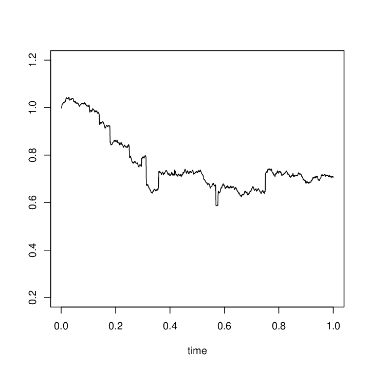
The organization of this paper is as follows. In Section 2.2, we introduce the α\alpha-quasi-log likelihood function ℍn​(θ,α){\mathbb{H}}_{n}(\theta;\alpha), that is a truncated version of the quasi-log likelihood function made from local Gaussian approximation, based on the global filter for the tuning parameter α\alpha. The α\alpha-quasi-maximum likelihood estimator (α\alpha-QMLE) θ^nM,α\hat{\theta}^{M,\alpha}_{n} is defined with respect to ℍn​(θ,α){\mathbb{H}}_{n}(\theta;\alpha). Since the truncation is formulated by the order statistics of the increments, this filter destroys adaptivity and martingale structure. However, the global filtering lemmas in Section 2.4 enable us to recover these properties. Section 2.5 gives a rate of convergence of the α\alpha-QMLE θ^nM,α\hat{\theta}^{M,\alpha}_{n} in LpL^{p} sense. In order to prove it, with the help of the QLA theory (Yoshida [16]), the so-called polynomial type large deviation inequality is derived in Theorem 2.13 for an annealed version of the quasi-log likelihood ℍnβ​(θ,α){\mathbb{H}}_{n}^{\beta}(\theta;\alpha) of (2.11), where β\beta is the annealing index. Moreover, the (α,β)(\alpha,\beta)-quasi-Bayesian estimator ((α,β)(\alpha,\beta)-QBE) θ^nB,α,β\hat{\theta}^{B,\alpha,\beta}_{n} can be defined as the Bayesian estimator with respect to ℍnβ​(θ,α){\mathbb{H}}_{n}^{\beta}(\theta;\alpha) as (2.12). Then the polynomial type large deviation inequality makes it possible to prove LpL^{p}-boundedness of the error of the (α,β)(\alpha,\beta)-QBE θ^nB,α,β\hat{\theta}^{B,\alpha,\beta}_{n} (Proposition 2.15). The α\alpha-QMLE and (α,β)(\alpha,\beta)-QBE do not attain the optimal rate of convergence when the parameter α\alpha is fixed though the fixed α\alpha-method surely removes jumps as a matter of fact. In Section 3, we introduce a quasi-likelihood function ℍn​(θ){\mathbb{H}}_{n}(\theta) depending on a moving level αn\alpha_{n}. The random field ℍn​(θ){\mathbb{H}}_{n}(\theta) is more aggressive than ℍn​(θ,α){\mathbb{H}}_{n}(\theta;\alpha) with a fixed α\alpha. Then a polynomial type large deviation inequality is obtained in Theorem 3.3 but the scaling factor is n−1/2n^{-1/2} in this case so that we can prove n\sqrt{n}-consistency in LpL^{p} sense for both QMLE θ^nM,αn\hat{\theta}^{M,\alpha_{n}}_{n} and QBE θ^nB,αn\hat{\theta}^{B,\alpha_{n}}_{n} associated with the random field ℍn​(θ){\mathbb{H}}_{n}(\theta) (Proposition 3.4). Stable convergence of these estimators and moment convergence are validated by Theorem 3.13. The moving threshold method attains the optimal rate of convergence in contrast to the fixed-α\alpha method. However, the theory requires the sequence αn\alpha_{n} should keep a certain balance: too large αn\alpha_{n} causes deficiency and too small αn\alpha_{n} may fail to filter out jumps. To balance efficiency of estimation and precision in filtering by taking advantage of the stability of the fixed-α\alpha scheme, in Section 4, we construct a one-step estimator θˇnM,α\check{\theta}^{M,\alpha}_{n} for a fixed α\alpha and the aggressive ℍn​(θ){\mathbb{H}}_{n}(\theta) with the α\alpha-QMLE θ^nM,α\hat{\theta}^{M,\alpha}_{n} as the initial estimator. Similarly, the one-step estimator θˇnB,α,β\check{\theta}^{B,\alpha,\beta}_{n} is constructed for fixed (α,β)(\alpha,\beta) and ℍn​(θ){\mathbb{H}}_{n}(\theta) with the (α,β)(\alpha,\beta)-quasi-Bayesian estimator θ^nB,α,β\hat{\theta}^{B,\alpha,\beta}_{n} for the initial estimator. By combining the results in Sections 2 and 3, we show that these estimators enjoy the same stable convergence and moment convergence as QMLE θ^nM,αn\hat{\theta}^{M,\alpha_{n}}_{n} and QBE θ^nB,αn\hat{\theta}^{B,\alpha_{n}}_{n}. It turns out in Section 6 that the so-constructed estimators are accurate and quite stable against α\alpha, in practice. In Section 5, we relax the conditions for stable convergence by a localization argument. Section 6 presents some simulation results and shows that the global filter can detect jumps more precisely than the local threshold methods.

2 Global filter: α\alpha-threshold method

2.1 Model structure

We will work with the model (1.1). To structure the model suitably, we begin with an example.

Example 2.1.

Consider a two-dimensional stochastic differential equation partly having jumps:

{d​ξt=btξ​d​t+σξ​(ξt,ηt,ζt,θ)​d​wtξ+d​Jtξd​ηt=btη​d​t+ση​(ξt,ηt,ζt,θ)​d​wtη.\displaystyle\left\{\begin{array}[]{ccl}d\xi_{t}&=&b_{t}^{\xi}dt+\sigma^{\xi}(\xi_{t},\eta_{t},\zeta_{t},\theta)dw^{\xi}_{t}+dJ^{\xi}_{t}\\ d\eta_{t}&=&b_{t}^{\eta}dt+\sigma^{\eta}(\xi_{t},\eta_{t},\zeta_{t},\theta)dw^{\eta}_{t}.\end{array}\right.

We can set Y=(ξ,η)Y=(\xi,\eta), X=(ξ,η,ζ)X=(\xi,\eta,\zeta) and J=(Jξ,0)J=(J^{\xi},0). No jump filter is necessary for the component η\eta.

This example suggests that different treatments should be given component-wise. We assume that

σ=diag​[σ(1)​(x,θ),…,σ(𝗄)​(x,θ)]\displaystyle\sigma=\text{diag}[\sigma^{({\color[rgb]{0,0,0}1})}(x,\theta),\ldots,\sigma^{({\sf k})}(x,\theta)]

for some 𝗆k×𝗆k{\sf m}_{k}\times{\sf m}_{k} nonnegative symmetric matrices σ(k)​(x,θ)\sigma^{(k)}(x,\theta), k=1,…,𝗄k=1,...,{\sf k}, and we further assume that w=(w(k))k=1,…,𝗄w=(w^{(k)})_{k=1,...,{\sf k}} with 𝗋=∑k=1𝗆𝗆k=𝗆{\sf r}={\color[rgb]{0,0,0}\sum_{k=1}^{\sf m}}{\sf m}_{k}={\sf m}. Let S=σ⊗2=σ​σ⋆S=\sigma^{\otimes 2}=\sigma\sigma^{\star}. Then S⁡(x,θ)S(x,\theta) has the form of

S⁡(x,θ)=diag​[S(1)​(x,θ),…,S(𝗄)​(x,θ)]\displaystyle S(x,\theta)=\text{diag}\big[S^{(1)}(x,\theta),...,S^{({\sf k})}(x,\theta)\big]

for 𝗆k×𝗆k{\sf m}_{k}\times{\sf m}_{k} matrices S(k)​(x,θ)=σ(k)​(σ(k))⋆​(x,θ)S^{(k)}(x,\theta){\color[rgb]{0,0,0}=\sigma^{(k)}(\sigma^{(k)})^{\star}(x,\theta)}, k=1,…,𝗄k=1,...,{\sf k}. According to the blocks of SS, we write

Yt=[Yt(1)Yt(𝗄)],bt=[bt(1)bt(𝗄)],wt=[wt(1)wt(𝗄)],Jt=[Jt(1)Jt(𝗄)].\displaystyle Y_{t}\>=\>\begin{bmatrix}Y^{(1)}_{t}\\ \vdots\\ Y^{({\sf k})}_{t}\end{bmatrix},\qquad b_{t}\>=\>\begin{bmatrix}b^{(1)}_{t}\\ \vdots\\ b^{({\sf k})}_{t}\end{bmatrix},\qquad w_{t}\>=\>\begin{bmatrix}w^{(1)}_{t}\\ \vdots\\ w^{({\sf k})}_{t}\end{bmatrix},\qquad J_{t}\>=\>\begin{bmatrix}J^{(1)}_{t}\\ \vdots\\ J^{({\sf k})}_{t}\end{bmatrix}.

Let NXt=∑s≤t1{ΔXs≠0}N^{X}_{t}=\sum_{s\leq t}1_{\{\Delta X_{s}\not=0\}}. We will pose a condition that NTX<∞N^{X}_{T}<\infty a.s. The jump part JXJ^{X} of XX is defined by JtX=∑s≤tΔ​XsJ^{X}_{t}=\sum_{s\leq t}\Delta X_{s}.

2.2 Quasi likelihood function by order statistics

In this section, we will give a filter that removes Δ​J\Delta J. [11] and [6] used certain jump detecting filters that cut large increments Δj​Y\Delta_{j}Y by a threshold comparable to diffusion increments. It is a local filter because the classification is done for each increment without using other increments. Contrarily, in this paper, we propose a global filter that removes increments Δj​Y\Delta_{j}Y when |Δj​Y||\Delta_{j}Y| is in an upper class among all data {|Δi​Y|}i=1,…,n\{|\Delta_{i}Y|\}_{i=1,...,n}.

We prepare statistics S¯n,j−1(k)\bar{S}^{(k)}_{n,j-1} (k=1,…,𝗄k=1,...,{\sf k}; j=1,…,nj=1,...,n; n∈ℕn\in{\mathbb{N}}) such that each S¯n,j−1(k)\bar{S}^{(k)}_{n,j-1} is an initial estimator of S(k)​(Xtj−1,θ∗)S^{(k)}(X_{t_{j-1}},\theta^{*}) up to a scaling constant, that is, there exists a (possibly unknown) positive constant c(k)c^{(k)} such that every S(k)​(Xtj−1,θ∗)S^{(k)}(X_{t_{j-1}},\theta^{*}) is approximated by c(k)​S¯n,j−1(k)c^{(k)}\bar{S}^{(k)}_{n,j-1}, as precisely stated later. We do not assume that S¯n,j−1(k)\bar{S}^{(k)}_{n,j-1} is ℱtj−1{\cal F}_{t_{j-1}}-measurable.

Example 2.2.

Let KK be a positive integer. Let (i¯n)(\bar{i}_{n}) be a diverging sequence of positive integers, e.g., i¯n∼h−1/2\bar{i}_{n}\sim h^{-1/2}. Let

S^n,j−1(k)\displaystyle\hat{S}^{(k)}_{n,j-1} =\displaystyle= ∑i=−i¯ni¯n(Δj−iY(k))⊗21{|Δj−i−K+1Y(k)|∧⋯∧|Δj−i−1Y(k)|≥|Δj−iY(k)|}hmax{1,∑i=−i¯ni¯n1{|Δj−i−K+1Y(k)|∧⋯∧|Δj−i−1Y(k)|≥|Δj−iY(k)|}}.\displaystyle\frac{\sum_{i=-\bar{i}_{n}}^{\bar{i}_{n}}\big(\Delta_{j-i}Y^{(k)}\big)^{\otimes 2}1_{\big\{|\Delta_{j-i-K+1}Y^{(k)}|\wedge\cdots\wedge|\Delta_{j-i-1}Y^{(k)}|\geq|\Delta_{j-i}Y^{(k)}|\big\}}}{h\max\bigg\{1,\sum_{i=-\bar{i}_{n}}^{\bar{i}_{n}}1_{\big\{|\Delta_{j-i-K+1}Y^{(k)}|\wedge\cdots\wedge|\Delta_{j-i-1}Y^{(k)}|\geq|\Delta_{j-i}Y^{(k)}|\big\}}\bigg\}}.

Here Δj​Y(k)\Delta_{j}Y^{(k)} reads 00 when j≤0j\leq 0 or j>nj>n. An example of S¯n,j−1(k)\bar{S}^{(k)}_{n,j-1} is

S¯n,j−1(k)\displaystyle\bar{S}^{(k)}_{n,j-1} =\displaystyle= S^(k)n,j−11{λm​i​n(S^(k)n,j−1)>2−1ϵ0}+2−1ϵ0I𝗆k1{λm​i​n(S^(k)n,j−1)≤2−1ϵ0},\displaystyle\hat{S}^{(k)}_{n,j-1}1_{\{\lambda_{min}(\hat{S}^{(k)}_{n,j-1})>2^{-1}\epsilon_{0}\}}+2^{-1}\epsilon_{0}{\color[rgb]{0,0,0}I_{{\sf m}_{k}}}1_{\{\lambda_{min}(\hat{S}^{(k)}_{n,j-1})\leq 2^{-1}\epsilon_{0}\}}, (2.2)

suppose that infx,θλm​i​n​(S(k)​(x,θ))≥ϵ0\displaystyle\inf_{x,\theta}\lambda_{min}(S^{(k)}(x,\theta))\geq\epsilon_{0} for some positive constant ϵ0\epsilon_{0}, where λm​i​n\lambda_{min} is the minimum eigenvalue of the matrix.

Let α=(α(k))k∈{1,…,𝗄}∈[0,1)𝗄\alpha=(\alpha^{(k)})_{k\in{\color[rgb]{0,0,0}\{1,\ldots,{\sf k}\}}}\in[0,1)^{\sf k}. Our global jump filter is constructed as follows. Denote by 𝒥n(k)​(α(k)){\cal J}_{n}^{(k)}(\alpha^{(k)}) the set of j∈{1,…,n}j\in\{1,...,n\} such that

#{j′∈{1,…,n};|(S¯n,j′−1(k))−1/2Δj′Y(k)|>|(S¯n,j−1(k))−1/2ΔjY(k)|}\displaystyle\#\big\{j^{\prime}\in\{1,...,n\};\>|(\bar{S}^{(k)}_{n,j^{\prime}-1})^{-1/2}\Delta_{j^{\prime}}Y^{(k)}|{\color[rgb]{0,0,0}>}|(\bar{S}^{(k)}_{n,j-1})^{-1/2}\Delta_{j}Y^{(k)}|\big\} ≥\displaystyle\geq α(k)​n\displaystyle\alpha^{(k)}n

for k=1,…,𝗄k=1,...,{\sf k} and n∈ℕn\in{\mathbb{N}}. If α(k)=0\alpha^{(k)}=0, then 𝒥n(k)(α(k))={1,….,n}{\cal J}_{n}^{(k)}(\alpha^{(k)})=\{1,....,n\}, that is, there is no filter for the kk-th component. The density function of the multi-dimensional normal distribution with mean vector μ\mu and covariance matrix CC is denoted by ϕ⁡(z,μ,C)\phi(z;\mu,C). Let

q(k)​(α(k))\displaystyle q^{(k)}(\alpha^{(k)}) =\displaystyle= Tr(∫{|z|≤c(α(k))1/2}z⊗2ϕ(z;0,I𝗆k)dz)Tr​(∫ℝ𝗆kz⊗2​ϕ​(z,0,I𝗆k)​𝑑z),\displaystyle\frac{\text{Tr}\bigg(\int_{\{|z|\leq c(\alpha^{(k)})^{1/2}\}}z^{\otimes 2}\phi(z;0,{\color[rgb]{0,0,0}I_{{\sf m}_{k}}})dz\bigg)}{\text{Tr}\bigg(\int_{{\mathbb{R}}^{{\color[rgb]{0,0,0}{\sf m}_{k}}}}z^{\otimes 2}\phi(z;0,{\color[rgb]{0,0,0}I_{{\sf m}_{k}}})dz\bigg)},

equivalently,

q(k)​(α(k))\displaystyle q^{(k)}(\alpha^{(k)}) =\displaystyle= (𝗆k)−1Tr(∫{|z|≤c(α(k))1/2}z⊗2ϕ(z;0,I𝗆k)dz)\displaystyle({\color[rgb]{0,0,0}{\sf m}_{k}})^{-1}\text{Tr}\bigg(\int_{\{|z|\leq c(\alpha^{(k)})^{1/2}\}}z^{\otimes 2}\phi(z;0,{\color[rgb]{0,0,0}I_{{\sf m}_{k}}})dz\bigg)
=\displaystyle= (𝗆k)−1E[V1{V≤c(α(k))}],\displaystyle({\sf m}_{k})^{-1}E[V1_{\{V\leq c(\alpha^{(k)})\}}],\quad

for a random variable V∼χ2​(𝗆k)V\sim\chi^{2}({{\sf m}_{k}}), the chi-squared distribution with 𝗆k{\color[rgb]{0,0,0}{\sf m}_{k}} degrees of freedom, where c⁡(α(k))c(\alpha^{(k)}) is determined by

P[V≤c(α(k))]\displaystyle P[V\leq c(\alpha^{(k)})] =\displaystyle= 1−α(k).\displaystyle 1-\alpha^{(k)}.

Let p⁡(α(k))=1−α(k)p(\alpha^{(k)})=1-\alpha^{(k)}. Now the 𝜶{\bm{\alpha}}-quasi-log likelihood function ℍn​(θ,α){\mathbb{H}}_{n}(\theta;\alpha) is defined by

ℍn​(θ,α)\displaystyle{\mathbb{H}}_{n}(\theta;\alpha) =\displaystyle= −12∑k=1𝗄∑j∈𝒥n(k)​(α(k)){q(k)(α(k))−1h−1S(k)(Xtj−1,θ)−1[(ΔjY(k))⊗2]Kn,j(k)\displaystyle-\frac{1}{2}\sum_{k=1}^{\sf k}\sum_{j\in{\cal J}^{(k)}_{n}(\alpha^{(k)})}\bigg\{q^{(k)}(\alpha^{(k)})^{-1}h^{-1}S^{(k)}(X_{t_{j-1}},\theta)^{-1}\big[\big(\Delta_{j}Y^{(k)}\big)^{\otimes 2}\big]K^{(k)}_{n,j}
+p(α(k))−1logdetS(k)(Xtj−1,θ)}\displaystyle+p(\alpha^{(k)})^{-1}\log\det S^{(k)}(X_{t_{j-1}},\theta)\bigg\}

where

Kn,j(k)\displaystyle K^{(k)}_{n,j} =\displaystyle= 1{|ΔjY(k)|<C(k)∗n−14}\displaystyle 1_{\big\{|\Delta_{j}Y^{(k)}|<C^{(k)}_{*}n^{-\frac{1}{4}}\big\}} (2.3)

and C∗(k)C^{(k)}_{*} are arbitrarily given positive constants. For a tensor T=(Ti1,…,ik)i1,…,ikT=(T_{i_{1},...,i_{k}})_{i_{1},...,i_{k}}, we write

T⁡[x1,…,xk]\displaystyle T[x_{1},...,x_{k}] =\displaystyle= T[x1⊗⋯⊗xk]=∑i1,…,ikTi1,…,ikx1i1⋯xkik\displaystyle T[x_{1}\otimes\cdots\otimes x_{k}]\>=\>\sum_{i_{1},...,i_{k}}T_{i_{1},...,i_{k}}x_{1}^{i_{1}}\cdots x_{k}^{i_{k}}

for x1=(x1i1)i1x_{1}=(x_{1}^{i_{1}})_{i_{1}}, …, xk=(xkik)ikx_{k}=(x_{k}^{i_{k}})_{i_{k}}. We denote u⊗r=u⊗⋯⊗uu^{\otimes r}=u\otimes\cdots\otimes u (rr times). Brackets [][\ \ ] stand for a multilinear mapping. This notation also applies to tensor-valued tensors.

If α(k)=0\alpha^{(k)}=0, then 𝒥n(k)​(α(k))={1,…,n}{\cal J}^{(k)}_{n}(\alpha^{(k)}{\color[rgb]{0,0,0})}=\{1,...,n\}, c⁡(α(k))=+∞c(\alpha^{(k)})=+\infty, p(k)​(α(k))=1p^{(k)}(\alpha^{(k)})=1 and q(k)​(α(k))=1q^{(k)}(\alpha^{(k)})=1, so the kk-th component of ℍn​(θ,α){\mathbb{H}}_{n}(\theta;\alpha) essentially becomes the ordinary quasi-log likelihood function by local Gaussian approximation.

Remark 2.3.

(i) The cap Kn,j(k)K^{(k)}_{n,j} can be removed if a suitable condition is assumed for the big jump sizes of JJ, e.g., supt∈[0,T]|ΔJt|∈L∞​–=∩p>1Lp\sup_{t\in[0,T]}|\Delta J_{t}|\in L^{\infty\text{--}}{\color[rgb]{0,0,0}=\cap_{p>1}L^{p}}. It is also reasonable to use

Kn,j(k)\displaystyle K^{(k)}_{n,j} =\displaystyle= 1{|S¯n,j−1−1/2ΔjY(k)|<C(k)∗n−14}\displaystyle 1_{\big\{|\bar{S}_{n,j-1}^{-1/2}\Delta_{j}Y^{(k)}|<C^{(k)}_{*}n^{-\frac{1}{4}}\big\}}

if S¯n,j−1\bar{S}_{n,j-1} is uniformly L∞​–L^{\infty\text{--}}-bounded. In any case, the factor Kn,j(k)K^{(k)}_{n,j} only serves for removing the effects of too big jumps and the classification is practically never affected by it since the global filter puts a threshold of the order less than n−1/2lognn^{-1/2}\log n. As a matter of fact, the threshold of Kn,j(k)K^{(k)}_{n,j} is of order O(n−1/4)O(n^{-1/4}), that is far looser than the ordinary local filters, and the truncation is exercised only with exponentially small probability. On the other hand, the global filter puts no restrictive condition on the distribution of the size of small jumps, like vanishing at the origin or boundedness of the density of the jump sizes, as assumed for the local filters so far. It should be emphasized that the difficulties in jump filtering are focused on the treatments of small jumps that look like the Brownian increments. (ii) The symmetry of σ(k)​(x,θ)\sigma^{(k)}(x,\theta) is not restrictive because σ(k)(Xt,θ)dwt(k)=S(k)(Xt,θ)1/2⋅(S(k)(Xt,θ)−1/2σ(k)(Xt,θ)dwt(k))\sigma^{(k)}(X_{t},\theta)dw^{(k)}_{t}=S^{(k)}(X_{t},\theta)^{1/2}\cdot\big(S^{(k)}(X_{t},\theta)^{-1/2}\sigma^{(k)}(X_{t},\theta)dw^{(k)}_{t}\big). On the other hand, we could introduce an 𝗆k×𝗆k{\sf m}_{k}\times{\sf m}_{k} random matrix σ¯n,j−1(k)\bar{\sigma}^{(k)}_{n,j-1} approximating σ(k)​(Xtj−1,θ∗)\sigma^{(k)}(X_{t_{j-1}},\theta^{*}) up to scaling, and use (σ¯n,j−1(k))−1​Δj​Y(k)\big(\bar{\sigma}^{(k)}_{n,j-1}\big)^{-1}\Delta_{j}Y^{(k)} for (S¯n,j−1(k))−1/2ΔjY(k)\big(\bar{S}^{(k)}_{n,j-1}\big)^{-1/2}\Delta_{j}Y^{(k)}, in order to remove the assumption of symmetry.

The 𝜶\bm{\alpha}-quasi-maximum likelihood estimator of θ\theta (α\alpha-QMLE) is any measurable mapping θ^nM,α\hat{\theta}^{M,\alpha}_{n} characterized by

ℍn​(θ^nM,α,α)\displaystyle{\mathbb{H}}_{n}(\hat{\theta}^{M,\alpha}_{n};\alpha) =\displaystyle= maxθ∈Θ¯⁡ℍn​(θ,α).\displaystyle\max_{\theta\in\bar{\Theta}}{\mathbb{H}}_{n}(\theta{\color[rgb]{0,0,0};}\alpha).

We will identify an estimator of θ\theta, that is a measurable mapping of the data, with the pull-back of it to Ω\Omega since the aim of discussion here is to obtain asymptotic properties of the estimators’ distribution.

2.3 Assumptions

We assume Sobolev’s embedding inequality

supθ∈Θ|f⁡(θ)|\displaystyle\sup_{\theta\in\Theta}\big|f(\theta)\big| ≤\displaystyle\leq CΘ,p​{∑i=01∫Θ|∂θif⁡(θ)|p​𝑑θ}1/p(f∈C1​(Θ))\displaystyle C_{\Theta,p}\bigg\{\sum_{i=0}^{1}\int_{\Theta}\big|\partial_{\theta}^{i}f(\theta)\big|^{p}{\color[rgb]{0,0,0}d\theta}\bigg\}^{1/p}\qquad(f\in C^{1}(\Theta))

for a bounded open set Θ\Theta in ℝ𝗉{\mathbb{R}}^{\sf p}, where CΘ,pC_{\Theta,p} is a constant, p>𝗉p>{\sf p}. This inequality is valid, e.g., if Θ\Theta has a Lipschitz boundary. Denote by C↑a,b​(ℝ𝖽×Θ,ℝ𝗆⊗ℝ𝗋)C_{\uparrow}^{a,b}({\mathbb{R}}^{\sf d}\times\Theta;{\mathbb{R}}^{\sf m}\otimes{\mathbb{R}}^{\sf r}) the set of continuous functions f:ℝ𝖽×Θ→ℝ𝗆⊗ℝ𝗋f:{\mathbb{R}}^{\sf d}\times\Theta\to{\mathbb{R}}^{\sf m}\otimes{\mathbb{R}}^{\sf r} that have continuous derivatives ∂s1⋯∂sℓf\partial_{s_{1}}\cdots\partial_{s_{\ell}}f for all (s1,…,sℓ)∈{θ,x}ℓ(s_{1},...,s_{\ell})\in\{\theta,x\}^{\ell} such that #⁡{i∈{1,…,ℓ};si=x}≤a\#\{i\in\{1,...,\ell\};\>s_{i}=x\}\leq a and #⁡{i∈{1,…,ℓ};si=θ}≤b\#\{i\in\{1,...,\ell\};\>s_{i}=\theta\}\leq b, and each of these derivatives satisfies

supθ∈Θ|∂s1⋯∂sℓf(x,θ)|\displaystyle\sup_{\theta\in\Theta}\big|\partial_{s_{1}}\cdots\partial_{s_{\ell}}f(x,\theta)\big| ≤\displaystyle\leq C⁡(s1,…,sℓ)​(1+|x|C⁡(s1,…,sℓ))(x∈ℝ𝖽)\displaystyle C(s_{1},...,s_{\ell})\big(1+|x|^{C(s_{1},...,s_{\ell})}\big)\quad(x\in{\mathbb{R}}^{\sf d})

for some positive constant C⁡(s1,…,sℓ)C(s_{1},...,s_{\ell}). Let ‖V‖p=(E⁡[|V|p])1/p\|V\|_{p}=\big(E[|V|^{p}])^{1/p} for a vector-valued random variable VV and p>0p>0. Let Nt(k)=∑s≤t1{ΔJ(k)s≠0}N_{t}^{(k)}=\sum_{s\leq t}1_{\{\Delta J^{(k)}_{s}\not=0\}} and Nt=∑s≤t1{ΔJs≠0}N_{t}=\sum_{s\leq t}1_{\{\Delta J_{s}\not=0\}} We shall consider the following conditions. Let X~=X−JX\widetilde{X}=X-J^{X} for JX=∑s∈[0,⋅]Δ​XsJ^{X}=\sum_{s\in[0,\cdot]}\Delta X_{s}.

[F1​​

]κ (i) For every p>1p>1, supt∈[0,T]‖Xt‖p<∞\sup_{t\in[0,T]}\|X_{t}\|_{p}<\infty and there exists a constant C⁡(p)C(p) such that

‖X~t−X~s‖p≤C⁡(p)​|t−s|1/2(t,s∈[0,T]).\displaystyle\|{\color[rgb]{0,0,0}\widetilde{X}_{t}-\widetilde{X}_{s}}\|_{p}\leq C(p)|t-s|^{1/2}\qquad(t,s\in[0,T]).
(ii)

supt∈[0,T]‖bt‖p<∞\sup_{t\in[0,T]}\|b_{t}\|_{p}<\infty for every p>1p>1.

(iii)

σ∈C↑2,κ​(ℝ𝖽×Θ,ℝ𝗆⊗ℝ𝗋)\sigma\in C^{2,\kappa}_{\uparrow}({\mathbb{R}}^{\sf d}\times\Theta;{\mathbb{R}}^{{\sf m}}\otimes{\mathbb{R}}^{\sf r}), S⁡(Xt,θ)S(X_{t},\theta) is invertible a.s. for every θ∈Θ\theta\in\Theta, and
supt∈[0,T],θ∈Θ‖S​(Xt,θ)−1‖p<∞\sup_{t\in[0,T],\theta\in\Theta}\|S(X_{t},\theta)^{-1}\|_{p}<\infty for every p>1p>1.

(iv)

NT∈L∞​–N_{T}\in L^{\infty\text{--}} and NTX∈L∞​–N^{X}_{T}\in L^{\infty\text{--}}.

Let (κn)n∈ℕ(\kappa_{n})_{n\in{\mathbb{N}}} be a sequence of positive integers satisfying κn=O⁡(n1/2)\kappa_{n}=O(n^{1/2}) as n→∞n\to\infty. For j∈{1,…,n}j\in\{1,...,n\}, let In,j={i∈{1,…,n};|i−j|≤κn}I_{n,j}=\big\{i\in\{1,...,n\};\>|i-j|\leq\kappa_{n}\big\}. Let 𝙸n,j=∪i∈In,j[ti−1,ti]{\tt I}_{n,j}=\cup_{i\in I_{n,j}}[t_{i-1},t_{i}]. Define the index set 𝖫n(k){\sf L}_{n}^{(k)} by

𝖫n(k)\displaystyle{\sf L}_{n}^{(k)} =\displaystyle= {j∈{1,…,n};N(k)(𝙸n,j)+NX(𝙸n,j)≠0}.\displaystyle\big\{j\in\{1,...,n\};\>N^{(k)}({\tt I}_{n,j})+N^{X}({\tt I}_{n,j})\not=0\big\}.
[F2​​

] (i) S¯n,j−1(k)\bar{S}^{(k)}_{n,j-1} are symmetric, invertible and supn∈ℕmaxj=1,…,n⁡‖(S¯n,j−1(k))−1‖p<∞\displaystyle\sup_{n\in{\mathbb{N}}}\max_{j=1,...,n}\big\|(\bar{S}^{(k)}_{n,j-1})^{-1}\big\|_{p}<\infty for every p>1p>1 and k=1,…,𝗄k=1,...,{\sf k}.

(ii)

There exist positive constants γ0\gamma_{0} and c(k)c^{(k)} (k=1,…,𝗄k=1,...,{\sf k}) such that

supn∈ℕmaxj=1,…,nnγ0∥(S(k)(Xtj−1,θ∗)−c(k)S¯n,j−1(k))1{j∈(𝖫n(k))c}∥p\displaystyle\sup_{n\in{\mathbb{N}}}\max_{j=1,...,n}n^{\gamma_{0}}{\color[rgb]{0,0,0}\bigg\|\bigg(S^{(k)}(X_{t_{j-1}},\theta^{*})-c^{(k)}\bar{S}^{(k)}_{n,j-1}\bigg)1_{\{j\in({\sf L}_{n}^{(k)})^{c}\}}\bigg\|_{p}} <\displaystyle< ∞\displaystyle\infty

for every p>1p>1 and k=1,…,𝗄k=1,...,{\sf k}.

Remark 2.4.

In [F​2][F2] (ii), we assumed that there exists a positive constant c(k)c^{(k)} such that every S(k)​(Xtj−1,θ∗)S^{(k)}(X_{t_{j-1}},\theta^{*}) is approximated by c(k)​S¯n,j−1(k)c^{(k)}\bar{S}_{n,j-1}^{(k)}. In estimation of θ\theta, we only assume positivity of c(k)c^{(k)} but the values of them can be unknown since the function ℍn{\mathbb{H}}_{n} does not involve c(k)c^{(k)}. When S(k)​(Xtj−1,θ∗)S^{(k)}(X_{t_{j-1}},\theta^{*}) is a scalar matrix, Condition [F​2]{\color[rgb]{0,0,0}[F2]} is satisfied simply by S¯n,j−1(k)=I𝗆k\bar{S}^{(k)}_{n,j-1}=I_{{\color[rgb]{0,0,0}{\sf m}_{k}}}.

Remark 2.5.

The S¯n,j−1(k)\bar{S}^{(k)}_{n,j-1} given by (2.2) in Example 2.2 satisfies Condition [F​2]{\color[rgb]{0,0,0}[F2]} with γ0=1/4\gamma_{0}=1/4 if one takes i¯n∼h−1/2\bar{i}_{n}\sim h^{-1/2}. The constant c(k)c^{(k)} depends on the depth KK of the threshold. It is possible to give an explicit expression of c(k)c^{(k)} but not required by the condition.

2.4 Global filtering lemmas

The α\alpha-quasi-log likelihood function ℍn​(θ,α){\mathbb{H}}_{n}(\theta;\alpha) involves the summation regarding the index set 𝒥n(k)​(α(k)){\cal J}^{(k)}_{n}(\alpha^{(k)}). The global jump filter 𝒥n(k)​(α(k)){\cal J}^{(k)}_{n}(\alpha^{(k)}) avoids taking jumps but it completely destroys the martingale structure that the ordinary quasi-log likelihood function originally possessed, and without the martingale structure, we cannot follow a standard way to validate desirable asymptotic properties the estimator should have. However, it is possible to recover the martingale structure to some extent by deforming the global jump filter to a suitable deterministic filter. In this section, we will give several lemmas that enable such a deformation.

As before, α=(α(k))k=1,…,𝗄\alpha=(\alpha^{(k)})_{k=1,...,{\sf k}} is a fixed vector in [0,1)𝗄[0,1)^{\sf k}. We may assume that γ0∈(0,1/2]\gamma_{0}\in(0,1/2] in [F​2]{\color[rgb]{0,0,0}[F2]}. Let

Uj(k)\displaystyle U^{(k)}_{j} =\displaystyle= (c(k))−1/2h−1/2(S¯n,j−1(k))−1/2ΔjY(k)andWj(k)=h−1/2Δjw(k).\displaystyle(c^{(k)})^{-1/2}h^{-1/2}(\bar{S}^{(k)}_{n,j-1})^{-1/2}\Delta_{j}Y^{(k)}\quad\text{and}\quad W^{(k)}_{j}\>=\>h^{-1/2}\Delta_{j}w^{(k)}.

By [F​1]0[F1]_{0} and [F​2]{\color[rgb]{0,0,0}[F2]}, we have

supn∈ℕsupj=1,…,n∥Rj(k)1{j∈(𝖫n(k))c}∥p=O(n−γ0)\displaystyle\sup_{n\in{\mathbb{N}}}\sup_{j=1,...,n}\big\|R^{(k)}_{j}{\color[rgb]{0,0,0}1_{\{j\in({\sf L}_{n}^{(k)})^{c}\}}}\big\|_{p}\>=\>O(n^{-\gamma_{0}})

for every p>1p>1, where

Rj(k)=Uj(k)−Wj(k)−(c(k))−1/2h−1/2(S¯n,j−1(k))−1/2ΔjJ(k).\displaystyle R^{(k)}_{j}=U^{(k)}_{j}-W^{(k)}_{j}-(c^{(k)})^{-1/2}h^{-1/2}(\bar{S}^{(k)}_{n,j-1})^{-1/2}\Delta_{j}J^{(k)}.

Remark that A1/2=1π∫0∞λ−1/2A(λ+A)−1dλA^{1/2}=\frac{1}{\pi}\int_{0}^{\infty}\lambda^{-1/2}A(\lambda+A)^{-1}d\lambda for a positive-definite matrix AA.

Denote |Wj(k)||W^{(k)}_{j}| and |Uj(k)||U^{(k)}_{j}| by W¯j(k)\overline{W}^{(k)}_{j} and U¯j(k)\overline{U}^{(k)}_{j}, respectively. W¯(j)(k)\overline{W}^{(k)}_{(j)} denotes the jj-th ordered statistic of {W¯1(k),…,W¯n(k)}\{\overline{W}^{(k)}_{1},...,\overline{W}^{(k)}_{n}\}, and U¯(j)(k)\overline{U}^{(k)}_{(j)} denotes the jj-th ordered statistic of {U¯1(k),…,U¯n(k)}\{\overline{U}^{(k)}_{1},...,\overline{U}^{(k)}_{n}\}. The rank of W¯j(k)\overline{W}^{(k)}_{j} is denoted by r⁡(W¯j(k))r({\color[rgb]{0,0,0}\overline{W}^{(k)}_{j}}). Denote by qα(k)q_{\alpha^{(k)}} the α(k)\alpha^{(k)}-quantile of the distribution of W¯1(k)\overline{W}^{(k)}_{1}. The number qα(k)q_{\alpha^{(k)}} depends on 𝗆k{\sf m}_{k}.

Let 0<γ2<γ1<γ00<\gamma_{2}<\gamma_{1}<\gamma_{0}. Let an(k)=⌊α¯(k)​n−n1−γ2⌋a_{n}^{(k)}=\lfloor\bar{\alpha}^{(k)}n-n^{1-\gamma_{2}}\rfloor, where α¯(k)=1−α(k)=p⁡(α(k))\bar{\alpha}^{(k)}=1-\alpha^{(k)}=p(\alpha^{(k)}). Define the event Nn,j(k)N_{n,j}^{(k)} by

Nn,j(k)\displaystyle N_{n,j}^{(k)} =\displaystyle= {r(W¯j(k))≤an(k)−n1−γ2}∩{W¯(an(k))(k)−W¯j(k)<n−γ1}.\displaystyle\big\{r(\overline{W}^{(k)}_{j})\leq a_{n}^{(k)}-n^{1-\gamma_{2}}\big\}{\color[rgb]{0,0,0}\cap}\big\{\overline{W}^{(k)}_{{\color[rgb]{0,0,0}(a_{n}^{(k)})}}-\overline{W}^{(k)}_{j}<n^{-\gamma_{1}}\big\}.
Lemma 2.6.

Suppose that α(k)∈(0,1)\alpha^{(k)}\in(0,1). Then P⁡[⋃j=1,..,,nNn,j(k)]=O⁡(n−L)\displaystyle P{\color[rgb]{0,0,0}\Big[\bigcup}_{j=1,..,,n}N_{n,j}^{(k)}{\color[rgb]{0,0,0}\Big]}\>=\>O(n^{-L}) as n→∞n\to\infty for every L>0L>0.

Proof.

We have

P[W¯(an(k))(k)>qα¯(k)+n−γ1]\displaystyle P{\color[rgb]{0,0,0}\Big[}\overline{W}^{(k)}_{{\color[rgb]{0,0,0}(a_{n}^{(k)})}}>q_{\bar{\alpha}^{(k)}}+n^{-\gamma_{1}}{\color[rgb]{0,0,0}\Big]}
=\displaystyle= P[∑j=1n1{W¯(k)j≤qα¯(k)+n−γ1}<an(k)]\displaystyle P\bigg[\sum_{j=1}^{n}1_{\{\overline{W}^{(k)}_{j}\leq q_{\bar{\alpha}^{(k)}}+n^{-\gamma_{1}}\}}<a_{n}^{(k)}\bigg]
=\displaystyle= P[n−1/2∑j=1n{1{W¯(k)j≤qα¯(k)+n−γ1}−P[W¯j(k)≤qα¯(k)+n−γ1]}<−n12−γ1c(n)]\displaystyle P\bigg[n^{-1/2}\sum_{j=1}^{n}\bigg\{1_{\{\overline{W}^{(k)}_{j}\leq q_{\bar{\alpha}^{(k)}}+n^{-\gamma_{1}}\}}-P\big[\overline{W}^{(k)}_{j}\leq q_{\bar{\alpha}^{(k)}}+n^{-\gamma_{1}}\big]\bigg\}<-n^{\frac{1}{2}-\gamma_{1}}c(n)\bigg]
=\displaystyle= O⁡(n−L)\displaystyle O(n^{-L})

for every L>0L>0, where (c⁡(n))n∈ℕ(c(n))_{n\in{\mathbb{N}}} is a sequence of numbers such that infn∈ℕc⁡(n)>0\inf_{n\in{\mathbb{N}}}c(n)>0 (the existence of such c⁡(n)c(n) can be proved by the mean value theorem). The last equality in the above estimates is obtained by the following argument. For Aj={W¯j(k)≤qα¯(k)+n−γ1}A_{j}=\{\overline{W}^{(k)}_{j}\leq q_{\bar{\alpha}^{(k)}}+n^{-\gamma_{1}}\} and Zj=1Aj−P⁡[A1]Z_{j}=1_{A_{j}}-P[A_{1}], by the Burkholder-Davis-Gundy inequality, Jensen’s inequality and |Zj|≤1|Z_{j}|\leq 1, we obtain

P[n−1/2∑j=1nZj<−n12−γ1c(n)]\displaystyle P\bigg[n^{-1/2}\sum_{j=1}^{n}Z_{j}<-n^{\frac{1}{2}-\gamma_{1}}c(n)\bigg]  ∼<\stackrel{{\scriptstyle{\textstyle<}}}{{\sim}} n−2​p​(12−γ1)​c​(n)−2​p​E​[n−1​∑j=1n|Zj|2​p]\displaystyle{\color[rgb]{0,0,0}n^{-2p(\frac{1}{2}-\gamma_{1})}c(n)^{-2p}E\Bigg[n^{-1}\sum_{j=1}^{n}|Z_{j}|^{2p}\Bigg]}
=\displaystyle= O⁡(n−p⁡(1−2​γ1))\displaystyle O(n^{-{\color[rgb]{0,0,0}p(1-2\gamma_{1})}})

for every p>1p>1.

Let

Bn(k)={|W¯(an(k))(k)−qα¯(k)|>n−γ1}.\displaystyle B_{n}^{(k)}=\big\{\big|\overline{W}^{(k)}_{{\color[rgb]{0,0,0}(a_{n}^{(k)})}}-q_{\bar{\alpha}^{(k)}}\big|>n^{-\gamma_{1}}\big\}.

We can estimate P[W¯(an(k))(k)<qα¯(k)−n−γ1]P\big[\overline{W}^{(k)}_{{\color[rgb]{0,0,0}(a_{n}^{(k)})}}<q_{\bar{\alpha}^{(k)}}-n^{-\gamma_{1}}\big], and so we have

P⁡[Bn(k)]\displaystyle P\big[B_{n}^{(k)}\big] =\displaystyle= O⁡(n−L)\displaystyle O(n^{-L}) (2.4)

for every L>0L>0.

By definition, on the event Nn,j(k)∩(Bn(k))cN^{{\color[rgb]{0,0,0}(k)}}_{n,j}\cap(B_{n}^{(k)})^{c}, the number of data W¯j′(k)\overline{W}^{(k)}_{j^{\prime}} on the interval [qα¯(k)−2​n−γ1,qα¯(k)+2​n−γ1]\big[q_{\bar{\alpha}^{(k)}}-2n^{-\gamma_{1}},q_{\bar{\alpha}^{(k)}}+2n^{-\gamma_{1}}\big] is not less than n1−γ2n^{1-\gamma_{2}}. However,

P[∑j′=1n1{W¯(k)j′∈[qα¯(k)−2n−γ1,qα¯(k)+2n−γ1]}≥n1−γ2]\displaystyle P\bigg[\sum_{j^{\prime}=1}^{n}1_{\big\{\overline{W}^{(k)}_{j^{\prime}}\in\big[q_{\bar{\alpha}^{(k)}}-2n^{-\gamma_{1}},q_{\bar{\alpha}^{(k)}}+2n^{-\gamma_{1}}\big]\big\}}\geq n^{1-\gamma_{2}}\bigg] (2.5)
=\displaystyle= P[n−1+γ1∑j′=1n1{W¯(k)j′∈[qα¯(k)−2n−γ1,qα¯(k)+2n−γ1]}≥nγ1−γ2]\displaystyle P\bigg[n^{-1+\gamma_{1}}\sum_{j^{\prime}=1}^{n}1_{\big\{\overline{W}^{(k)}_{j^{\prime}}\in\big[q_{\bar{\alpha}^{(k)}}-2n^{-\gamma_{1}},q_{\bar{\alpha}^{(k)}}+2n^{-\gamma_{1}}\big]\big\}}\geq n^{\gamma_{1}-\gamma_{2}}\bigg]
=\displaystyle= O⁡(n−L)\displaystyle O(n^{-L})

for every L>0L>0. Indeed, the family

{n−1/2∑j′=1n(1{W¯(k)j′∈[qα¯(k)−2n−γ1,qα¯(k)+2n−γ1]}−E[1{W¯(k)j′∈[qα¯(k)−2n−γ1,qα¯(k)+2n−γ1]}])}n∈ℕ\displaystyle\bigg\{n^{-1/2}\sum_{j^{\prime}=1}^{n}\bigg(1_{\big\{\overline{W}^{(k)}_{j^{\prime}}\in\big[q_{\bar{\alpha}^{(k)}}-2n^{-\gamma_{1}},q_{\bar{\alpha}^{(k)}}+2n^{-\gamma_{1}}\big]\big\}}-E\bigg[1_{\big\{\overline{W}^{(k)}_{j^{\prime}}\in\big[q_{\bar{\alpha}^{(k)}}-2n^{-\gamma_{1}},q_{\bar{\alpha}^{(k)}}+2n^{-\gamma_{1}}\big]\big\}}\bigg]\bigg)\bigg\}_{n\in{\mathbb{N}}}

is bounded in L∞​–L^{\infty\text{--}} (this can be proved by the same argument as above). Since the estimate (2.5) is independent of j∈{1,…,n}j\in\{1,...,n\}, combining it with (2.4), we obtain

maxj=1,..,,n⁡P⁡[Nn,j(k)]=O⁡(n−L)\displaystyle\max_{j=1,..,,n}P\big[N_{n,j}^{(k)}\big]\>=\>O(n^{-L})

as n→∞n\to\infty for every L>0L>0. Now the desired inequality of the lemma is obvious. ∎

Let

𝒥^n(k)​(α(k))\displaystyle\hat{{\cal J}}_{n}^{(k)}(\alpha^{(k)}) =\displaystyle= {j∈{1,…,n};r⁡(W¯j(k))≤a^n(k)},\displaystyle\bigg\{j\in\{1,...,n\};\>r(\overline{W}^{(k)}_{j})\leq\hat{a}^{(k)}_{n}\bigg\},

where

a^n(k)\displaystyle\hat{a}^{(k)}_{n} =\displaystyle= ⌊an(k)−n1−γ2⌋.\displaystyle\lfloor a^{(k)}_{n}-n^{1-\gamma_{2}}\rfloor.

Let

Ωn\displaystyle\Omega_{n} =\displaystyle= {∑k#𝖫n(k)<n1−γ2}⋂(⋂k=1,…,𝗄⋂j=1,…,n[{|Rj(k)|1{j∈(𝖫n(k))c}<2−1n−γ1}∩(Nn,j(k))c]).\displaystyle{\color[rgb]{0,0,0}\bigg\{\sum_{k}\#{\sf L}_{n}^{(k)}<n^{1-\gamma_{2}}\bigg\}}{\color[rgb]{0,0,0}\bigcap}\bigg(\bigcap_{k=1,...,{\sf k}}\bigcap_{j=1,...,n}\bigg[\big\{|R^{(k)}_{j}|{\color[rgb]{0,0,0}1_{\{j\in({\sf L}_{n}^{(k)})^{c}\}}}<2^{-1}n^{-\gamma_{1}}\big\}\cap(N^{(k)}_{n,j})^{c}\bigg]\bigg).
Lemma 2.7.
𝒥^n(k)​(α(k))∩(𝖫n(k))c\displaystyle\hat{{\cal J}}_{n}^{(k)}(\alpha^{(k)})\cap({\color[rgb]{0,0,0}{\sf L}^{(k)}_{n}})^{c} ⊂\displaystyle\subset 𝒥n(k)​(α(k))\displaystyle{\cal J}^{(k)}_{n}(\alpha^{(k)}) (2.6)

on Ωn\Omega_{n}. In particular

#⁡[𝒥n(k)​(α(k))⊖𝒥^n(k)​(α(k))]\displaystyle\#\big[{\cal J}^{(k)}_{n}(\alpha^{(k)})\ominus\hat{{\cal J}}_{n}^{(k)}(\alpha^{(k)})\big] ≤\displaystyle\leq c∗​n1−γ2+#​𝖫n(k)\displaystyle c_{*}n^{1-\gamma_{2}}+{\color[rgb]{0,0,0}\#\>{\sf L}_{n}^{(k)}} (2.7)

on Ωn\Omega_{n}, where c∗c_{*} is a positive constant. Here ⊖\ominus denotes the symmetric difference operator of sets.

Proof.

On Ωn\Omega_{n}, if a pair (j1,j2)∈(𝖫n(k))c×(𝖫n(k))c(j_{1},j_{2})\in({\color[rgb]{0,0,0}{\sf L}^{(k)}_{n}})^{c}\times({\color[rgb]{0,0,0}{\sf L}^{(k)}_{n}})^{c} satisfies r⁡(W¯j1(k))≤a^n(k)r(\overline{W}^{(k)}_{j_{1}})\leq\hat{a}^{(k)}_{n} and r⁡(W¯j2(k))≥an(k)r(\overline{W}^{(k)}_{j_{2}})\geq a^{(k)}_{n}, then U¯j1(k)<W¯j1(k)+2−1​n−γ1≤W¯(an(k))(k)−2−1​n−γ1≤W¯j2(k)−2−1​n−γ1<U¯j2(k)\overline{U}^{(k)}_{j_{1}}<\overline{W}^{(k)}_{j_{1}}+2^{-1}n^{-\gamma_{1}}\leq\overline{W}^{(k)}_{(a^{(k)}_{n})}-2^{-1}n^{-\gamma_{1}}\leq\overline{W}^{(k)}_{j_{2}}-2^{-1}n^{-\gamma_{1}}<\overline{U}^{(k)}_{j_{2}}. Therefore, if j∈𝒥^n(k)​(α(k))∩(𝖫n(k))cj\in\hat{{\cal J}}^{(k)}_{n}(\alpha^{(k)})\cap({\color[rgb]{0,0,0}{\sf L}^{(k)}_{n}})^{c}, then j∈𝒥n(k)​(α(k))j\in{\cal J}^{(k)}_{n}(\alpha^{(k)}) since one can find at least ⌈α(k)​n⌉(≤(n−an(k)+1)−n1−γ2)\lceil\alpha^{(k)}n\rceil{\color[rgb]{0,0,0}(\leq(n-a^{(k)}_{n}+1)-n^{1-\gamma_{2}})} variables among U¯(an(k))(k),…..,U¯(n)(k)\overline{U}^{(k)}_{(a_{n}^{(k)})},.....,\overline{U}^{(k)}_{(n)} that are larger than U¯j(k)\overline{U}^{(k)}_{j}. Therefore (2.6) holds, and so does (2.7) as follows. From (2.6), we have #⁡[𝒥n(k)​(α(k))⊖𝒥^n(k)​(α(k))]≤𝖭+#​𝖫n(k)\#\big[{\cal J}^{(k)}_{n}(\alpha^{(k)})\ominus\hat{{\cal J}}_{n}^{(k)}(\alpha^{(k)})\big]\leq{\sf N}+{\color[rgb]{0,0,0}\#\>{\sf L}^{(k)}_{n}} for

𝖭\displaystyle{\sf N} =\displaystyle= #⁡[𝒥n(k)​(α(k))∩𝒥^n(k)​(α(k))c∩(𝖫n(k))c].\displaystyle\#\big[{\cal J}^{(k)}_{n}(\alpha^{(k)})\cap\hat{{\cal J}}_{n}^{(k)}(\alpha^{(k)})^{c}\cap({\color[rgb]{0,0,0}{\sf L}_{n}^{(k)}})^{c}\big].

Suppose that j∈𝒥n(k)​(α(k))∩𝒥^n(k)​(α(k))c∩(𝖫n(k))cj\in{\cal J}^{(k)}_{n}(\alpha^{(k)})\cap\hat{{\cal J}}_{n}^{(k)}(\alpha^{(k)})^{c}\cap({\color[rgb]{0,0,0}{\sf L}_{n}^{(k)}})^{c}. In Case r⁡(W¯j(k))<an(k)r(\overline{W}^{(k)}_{j})<a^{(k)}_{n}, since a^n(k)<r⁡(W¯j(k))<an(k)\hat{a}^{(k)}_{n}<r(\overline{W}^{(k)}_{j})<a^{(k)}_{n}, we know the number of such jj is less than or equal to n1−γ2n^{1-\gamma_{2}}. In Case r⁡(W¯j(k))≥an(k)r(\overline{W}^{(k)}_{j})\geq a^{(k)}_{n}, as seen above, U¯j1(k)<U¯j(k)\overline{U}^{(k)}_{j_{1}}<\overline{U}^{(k)}_{j} on Ωn\Omega_{n} for all j1∈(𝖫n(k))cj_{1}\in({\color[rgb]{0,0,0}{\sf L}_{n}^{(k)}})^{c} satisfying r⁡(W¯j1(k))≤a^n(k)r(\overline{W}^{(k)}_{j_{1}})\leq\hat{a}^{(k)}_{n}, since j∈(𝖫n(k))cj\in({\color[rgb]{0,0,0}{\sf L}_{n}^{(k)}})^{c} and r⁡(W¯j(k))≥an(k)r(\overline{W}^{(k)}_{j}){\color[rgb]{0,0,0}\>\geq\>}a^{(k)}_{n}. The number of such j1j_{1}s is at least a^n(k)−⌊n1−γ2⌋\hat{a}^{(k)}_{n}-\lfloor n^{1-\gamma_{2}}\rfloor. On the other hand, j∈𝒥n(k)​(α(k))j\in{\cal J}^{(k)}_{n}(\alpha^{(k)}) gives #⁡{j′∈{1,…,n};U¯j(k)<U¯j′(k)}≥⌈α(k)​n⌉\#\{j^{\prime}\in\{1,...,n\};\>\overline{U}^{(k)}_{j}<\overline{U}^{(k)}_{j^{\prime}}\}\geq\lceil\alpha^{(k)}n\rceil. Therefore

𝖭\displaystyle{\sf N} ≤\displaystyle\leq n1−γ2+n−(a^n(k)−⌊n1−γ2⌋)−⌈α(k)​n⌉≤ 4​n1−γ2+2\displaystyle{\color[rgb]{0,0,0}n^{1-\gamma_{2}}+}n-\big(\hat{a}^{(k)}_{n}-\lfloor n^{1-\gamma_{2}}\rfloor\big)-\lceil\alpha^{(k)}n\rceil\>\leq\>{\color[rgb]{0,0,0}4}n^{1-\gamma_{2}}+{\color[rgb]{0,0,0}2}

on Ωn\Omega_{n}. We obtain (2.7) on Ωn\Omega_{n} with c∗=6c_{*}={\color[rgb]{0,0,0}6} if we use the inequality 4​n1−γ2+2≤6​n1−γ2{\color[rgb]{0,0,0}4}n^{1-\gamma_{2}}+{\color[rgb]{0,0,0}2}\leq{\color[rgb]{0,0,0}6}n^{1-\gamma_{2}}. ∎

Let γ3>0\gamma_{3}>0. For random variables (Vj)j=1,…,n(V_{j})_{j=1,...,n}, let

𝒟n(k)\displaystyle{\cal D}_{n}^{(k)} =\displaystyle= nγ3​|1n​∑j∈𝒥n(k)​(α(k))Vj−1n​∑j∈𝒥^n(k)​(α(k))Vj|.\displaystyle n^{\gamma_{3}}{\color[rgb]{0,0,0}\Bigg|}\frac{1}{n}\sum_{j\in{\cal J}^{(k)}_{n}(\alpha^{(k)})}V_{j}-\frac{1}{n}\sum_{j\in\hat{{\cal J}}^{(k)}_{n}(\alpha^{(k)})}V_{j}{\color[rgb]{0,0,0}\Bigg|}.
Lemma 2.8.

(i) Let p1>1p_{1}>1. Then

‖𝒟n(k)‖p\displaystyle\|{\cal D}_{n}^{(k)}\|_{p} ≤\displaystyle\leq (c∗​nγ3−γ2+n−1+γ3​‖#​𝖫n(k)‖p1)​‖maxj=1,…,n⁡|Vj|‖p​p1​(p1−p)−1\displaystyle\big(c_{*}n^{\gamma_{3}-\gamma_{2}}+n^{-1+\gamma_{3}}\|{\color[rgb]{0,0,0}\#\>{\sf L}_{n}^{(k)}}\|_{p_{1}}\big)\bigg\|\max_{j=1,...,n}\big|V_{j}\big|\bigg\|_{pp_{1}(p_{1}-p)^{-1}}
+nγ3​‖maxj=1,…,n⁡|Vj|​1Ωnc‖p\displaystyle+n^{\gamma_{3}}\bigg\|\max_{j=1,...,n}\big|V_{j}\big|1_{\Omega_{n}^{c}}\bigg\|_{p}

for p∈(1,p1)p\in(1,p_{1}).

(ii)

Let γ4>0\gamma_{4}>0 and p1>1p_{1}>1. Then

‖𝒟n(k)‖p\displaystyle\|{\cal D}_{n}^{(k)}\|_{p} ≤\displaystyle\leq (c∗​nγ3−γ2+n−1+γ3​‖#​𝖫n(k)‖p1)\displaystyle\big(c_{*}n^{\gamma_{3}-\gamma_{2}}+n^{-1+\gamma_{3}}\|{\color[rgb]{0,0,0}\#\>{\sf L}_{n}^{(k)}}\|_{p_{1}}\big)
×(nγ4+nmaxj=1,…,n∥|Vj|1{|Vj|>nγ4}∥p​p1​(p1−p)−1)\displaystyle\times\bigg(n^{\gamma_{4}}+n\max_{j=1,...,n}\bigg\|\big|V_{j}\big|1_{\{|V_{j}|>n^{\gamma_{4}}\}}\bigg\|_{pp_{1}(p_{1}-p)^{-1}}\bigg)
+nγ3​‖maxj=1,…,n⁡|Vj|​1Ωnc‖p\displaystyle+n^{\gamma_{3}}\bigg\|\max_{j=1,...,n}\big|V_{j}\big|1_{\Omega_{n}^{c}}\bigg\|_{p}

for p∈(1,p1)p\in(1,p_{1}).

Proof.

The estimate in (i) is obvious from (2.7). (ii) follows from (i). ∎

Let 𝒥~n(k)(α(k))={j;|h−1/2Δjw(k)|≤qα¯(k)}={j;W¯j(k)≤qα¯(k)}\widetilde{{\cal J}}^{(k)}_{n}(\alpha^{(k)})=\big\{j;\>|h^{-1/2}\Delta_{j}w^{(k)}|\leq q_{\bar{\alpha}^{(k)}}\big\}{=\color[rgb]{0,0,0}\big\{j;\>\overline{W}^{(k)}_{j}\leq q_{\bar{\alpha}^{(k)}}\big\}}. Let

𝒟~n(k)\displaystyle\tilde{{\cal D}}_{n}^{(k)} =\displaystyle= nγ3​|1n​∑j∈𝒥^n(k)​(α(k))Vj−1n​∑j∈𝒥~n(k)​(α(k))Vj|.\displaystyle n^{\gamma_{3}}\bigg|\frac{1}{n}\sum_{j\in\hat{{\cal J}}^{(k)}_{n}(\alpha^{(k)})}V_{j}-\frac{1}{n}\sum_{j\in\widetilde{{\cal J}}^{(k)}_{n}(\alpha^{(k)})}V_{j}\bigg|.
Lemma 2.9.

Let Ω~n={|W¯(a^n(k))(k)−qα¯(k)|<Cˇn−γ2}\tilde{\Omega}_{n}=\big\{\big|\overline{W}^{(k)}_{(\hat{a}^{(k)}_{n})}-q_{\bar{\alpha}^{(k)}}\big|<{\color[rgb]{0,0,0}\check{C}\>}n^{-\gamma_{2}}\big\}, where Cˇ\check{C} is a positive constant. Then

(i)

For p≥1p\geq 1,

‖𝒟~n(k)‖p\displaystyle\|\tilde{{\cal D}}_{n}^{(k)}\|_{p} ≤\displaystyle\leq nγ3∥maxj′=1,…,n|Vj′|1n∑j=1n1{|W¯(k)j−qα¯(k)|≤Cˇn−γ2}∥p+nγ3∥1Ω~ncmaxj′=1,…,n|Vj′|∥p.\displaystyle n^{\gamma_{3}}\bigg\|\max_{j^{\prime}=1,...,n}|V_{j^{\prime}}|\>\frac{1}{n}\sum_{j=1}^{n}1_{\big\{\big|\overline{W}^{(k)}_{j}-q_{\bar{\alpha}^{(k)}}\big|\leq{\color[rgb]{0,0,0}\check{C}\>}n^{-\gamma_{2}}\big\}}\bigg\|_{p}+n^{\gamma_{3}}\bigg\|1_{\tilde{\Omega}_{n}^{c}}\max_{j^{\prime}=1,...,n}|V_{j^{\prime}}|\bigg\|_{p}.
(ii)

For p1>p≥1p_{1}>p\geq 1,

‖𝒟~n(k)‖p\displaystyle\|\tilde{{\cal D}}_{n}^{(k)}\|_{p} ≤\displaystyle\leq nγ3∥maxj=1,…,n|Vj|∥pP[|W¯1(k)−qα¯(k)|≤Cˇn−γ2]\displaystyle n^{\gamma_{3}}\bigg\|\max_{j=1,...,n}|V_{j}|\>\bigg\|_{p}P\bigg[\big|\overline{W}^{(k)}_{1}-q_{\bar{\alpha}^{(k)}}\big|\leq{\color[rgb]{0,0,0}\check{C}\>}n^{-\gamma_{2}}\bigg]
+nγ3​‖maxj=1,…,n⁡|Vj|‖p​p1​(p1−p)−1\displaystyle+n^{\gamma_{3}}\bigg\|\max_{j=1,...,n}|V_{j}|\bigg\|_{pp_{1}(p_{1}-p)^{-1}}
×∥1n∑j=1n(1{|W¯(k)j−qα¯(k)|≤Cˇn−γ2}−P[|W¯1(k)−qα¯(k)|≤Cˇn−γ2])∥p1\displaystyle\hskip 30.0pt\times\bigg\|\frac{1}{n}\sum_{j=1}^{n}\bigg(1_{\big\{\big|\overline{W}^{(k)}_{j}-q_{\bar{\alpha}^{(k)}}\big|\leq{\color[rgb]{0,0,0}\check{C}\>}n^{-\gamma_{2}}\big\}}-P\bigg[\big|\overline{W}^{(k)}_{1}-q_{\bar{\alpha}^{(k)}}\big|\leq{\color[rgb]{0,0,0}\check{C}\>}n^{-\gamma_{2}}\bigg]\bigg)\bigg\|_{p_{1}}
+nγ3​P​[Ω~nc]1/p1​‖maxj=1,…,n⁡|Vj|‖p​p1​(p1−p)−1.\displaystyle+n^{\gamma_{3}}P[{\color[rgb]{0,0,0}\tilde{\Omega}}_{n}^{c}]^{1/p_{1}}\bigg\|\max_{j=1,...,n}|V_{j}|\bigg\|_{pp_{1}(p_{1}-p)^{-1}}.
Proof.

(i) follows from

1Ω~n|1{W¯(k)j≤W¯(k)(a^n(k))}−1{W¯(k)j≤qα¯(k)}|\displaystyle 1_{\tilde{\Omega}_{n}}\bigg|1_{\{\overline{W}^{(k)}_{j}\leq\overline{W}^{(k)}_{(\hat{a}_{n}^{(k)})}\}}-1_{\{\overline{W}^{(k)}_{j}\leq q_{\bar{\alpha}^{(k)}}\}}\bigg| ≤\displaystyle\leq 1{|W¯(k)j−qα¯(k)|≤Cˇn−γ2},\displaystyle 1_{\big\{\big|\overline{W}^{(k)}_{j}-q_{\bar{\alpha}^{(k)}}\big|\leq{\color[rgb]{0,0,0}\check{C}\>}n^{-\gamma_{2}}\big\}},

and (ii) follows from (i). ∎

We take a sufficiently large Cˇ\check{C}. Then the term involving Ω~nc\tilde{\Omega}_{n}^{c} on the right-hand side of each inequality in Lemma 2.9 can be estimated as the proof of Lemma 2.6. For example, P⁡[Ω~nc]=O⁡(n−L)P[\tilde{\Omega}_{n}^{c}]=O(n^{-L}) for any L>0L>0.

Lemma 2.10.

Let k∈{1,…,𝗄}k\in\{1,...,{\sf k}\} and let f∈C↑1,1​(ℝ𝖽×Θ,ℝ)f\in C^{1,1}_{\uparrow}\big({\mathbb{R}}^{\sf d}\times\Theta;{\mathbb{R}}). Suppose that [F​1]0{\color[rgb]{0,0,0}[F1]_{0}} is fulfilled. Then

supn∈ℕ‖supθ∈Θnϵ​|1n​∑j∈𝒥n(k)​(α(k))p​(α(k))−1​f​(Xtj−1,θ)−1T​∫0Tf⁡(Xt,θ)​𝑑t|‖p\displaystyle\sup_{n\in{\mathbb{N}}}\left\|\>\sup_{\theta\in\Theta}n^{\epsilon}\left|\frac{1}{n}\sum_{j\in{\cal J}^{(k)}_{n}(\alpha^{(k)})}p(\alpha^{(k)})^{-1}f(X_{t_{j-1}},\theta)-\frac{1}{T}\int_{0}^{T}f(X_{t},\theta)dt\right|\>\right\|_{p} <\displaystyle< ∞\displaystyle\infty

for every p≥1p\geq 1 and ϵ<γ2\epsilon<{\color[rgb]{0,0,0}\gamma_{2}} .

Proof.

Use Sobolev’s inequality and Burkholder’s inequality as well as Lemmas 2.6, 2.8 (ii) and 2.9 (ii). More precisely, we have the following decomposition

1n​∑j∈𝒥n(k)​(α(k))p​(α(k))−1​f​(Xtj−1,θ)−1T​∫0Tf⁡(Xt,θ)​𝑑t\displaystyle\frac{1}{n}\sum_{j\in{\cal J}^{(k)}_{n}(\alpha^{(k)})}{\color[rgb]{0,0,0}p(\alpha^{(k)})^{-1}}f(X_{t_{j-1}},\theta)-\frac{1}{T}\int_{0}^{T}f(X_{t},\theta)dt
=\displaystyle= p​(α(k))−1​{1n​∑j∈𝒥n(k)​(α(k))f⁡(Xtj−1,θ)−1n​∑j∈𝒥^n(k)​(α(k))f⁡(Xtj−1,θ)}\displaystyle p(\alpha^{(k)})^{-1}\left\{\frac{1}{n}\sum_{j\in{\cal J}^{(k)}_{n}(\alpha^{(k)})}f(X_{t_{j-1}},\theta)-\frac{1}{n}\sum_{j\in\hat{{\cal J}}^{(k)}_{n}(\alpha^{(k)})}f(X_{t_{j-1}},\theta)\right\}
+p​(α(k))−1​{1n​∑j∈𝒥^n(k)​(α(k))f⁡(Xtj−1,θ)−1n​∑j∈𝒥~n(k)​(α(k))f⁡(Xtj−1,θ)}\displaystyle+p(\alpha^{(k)})^{-1}\left\{\frac{1}{n}\sum_{j\in\hat{{\cal J}}^{(k)}_{n}(\alpha^{(k)})}f(X_{t_{j-1}},\theta)-\frac{1}{n}\sum_{j\in\tilde{{\cal J}}^{(k)}_{n}(\alpha^{(k)})}f(X_{t_{j-1}},\theta)\right\}
+1n​p​(α(k))∑j=1nf(Xtj−1,θ){1{W¯(k)j≤qα¯(k)}−p(α(k))}\displaystyle+\frac{1}{np(\alpha^{(k)})}\sum_{j=1}^{n}f(X_{t_{j-1}},\theta)\bigg\{1_{\big\{\overline{W}^{(k)}_{j}\leq{\color[rgb]{0,0,0}q_{\bar{\alpha}^{(k)}}}\big\}}-p(\alpha^{(k)})\bigg\}
+1n​h∑j=1n∫tj−1tj[f(Xtj−1,θ)−f(Xt,θ)]dt\displaystyle+\frac{1}{nh}\sum_{j=1}^{n}\int_{t_{j-1}}^{t_{j}}[f(X_{t_{j-1}},\theta)-f(X_{t},\theta)]dt
=:\displaystyle=: I1,n(k)​(θ)+I2,n(k)​(θ)+I3,n(k)​(θ)+I4,n(k)​(θ).\displaystyle I_{1,n}^{(k)}(\theta)+I_{2,n}^{(k)}(\theta)+I_{3,n}^{(k)}(\theta)+I_{4,n}^{(k)}(\theta).

We may assume α(k)>0\alpha^{(k)}>0 since only I4,n(k)​(θ)I^{(k)}_{4,n}(\theta) remains when α(k)=0\alpha^{(k)}=0 and it will be estimated below.

As for I1,n(k)​(θ)I_{1,n}^{(k)}(\theta), we apply Lemma 2.8 (ii) to obtain

‖supθ∈Θnϵ​|I1,n(k)​(θ)|‖p\displaystyle\Bigg\|\sup_{\theta\in\Theta}n^{\epsilon}{\color[rgb]{0,0,0}\big|}I_{1,n}^{(k)}(\theta){\color[rgb]{0,0,0}\big|}\Bigg\|_{p}  ∼<\stackrel{{\scriptstyle{\textstyle<}}}{{\sim}} ∑i=0,1supθ∈Θ‖nϵ​|1n​∑j∈𝒥n(k)​(α(k))∂θif⁡(Xtj−1,θ)−1n​∑j∈𝒥^n(k)​(α(k))∂θif⁡(Xtj−1,θ)|‖p\displaystyle{\color[rgb]{0,0,0}\sum_{i=0,1}\sup_{\theta\in\Theta}\left\|n^{\epsilon}\left|\frac{1}{n}\sum_{j\in{\cal J}^{(k)}_{n}(\alpha^{(k)})}\partial_{\theta}^{i}f(X_{t_{j-1}},\theta)-\frac{1}{n}\sum_{j\in\hat{{\cal J}}^{(k)}_{n}(\alpha^{(k)})}\partial_{\theta}^{i}f(X_{t_{j-1}},\theta)\right|\right\|_{p}}
 ∼<\stackrel{{\scriptstyle{\textstyle<}}}{{\sim}} ∑i=0,1supθ∈Θ{(c∗nϵ−γ2+n−1+ϵ∥#𝖫n(k)∥p1)\displaystyle{\color[rgb]{0,0,0}\color[rgb]{0,0,0}\sum_{i=0,1}\sup_{\theta\in\Theta}\Bigg\{}\Big(c_{*}n^{\epsilon-\gamma_{2}}+n^{-1+\epsilon}\|{\color[rgb]{0,0,0}\#\>{\sf L}_{n}^{(k)}}\|_{p_{1}}\Big)
×(nγ4+nmaxj∥|∂θif(Xtj−1,θ)|1{|∂θif(Xtj−1,θ)|≥nγ4}∥p​p1p1−p)\displaystyle\>\times\Bigg(n^{\gamma_{4}}+{\color[rgb]{0,0,0}n\max_{j}\Bigg\||\partial_{\theta}^{i}f(X_{t_{j-1}},\theta)|1_{\{|\partial_{\theta}^{i}f(X_{t_{j-1}},\theta)|\geq n^{\gamma_{4}}\}}\Bigg\|_{\frac{pp_{1}}{p_{1}-p}}}\Bigg)
+nϵ∥maxj|∂θif(Xtj−1,θ)|1Ωnc∥p}.\displaystyle{\color[rgb]{0,0,0}+n^{\epsilon}\Bigg\|\max_{j}|\partial_{\theta}^{i}f(X_{t_{j-1}},\theta)|1_{\Omega_{n}^{c}}\Bigg\|_{p}\Bigg\}.}

By taking γ4>0\gamma_{4}>0 small enough, we can verify that the right-hand side is o⁡(1)o(1) since

‖#​𝖫n(k)‖p∼<κn​‖NT+NTX‖p=O⁡(n1/2).\displaystyle\big\|\#\>{\sf L}_{n}^{(k)}\big\|_{p}\ \raisebox{-3.01385pt}{$\stackrel{{\scriptstyle{\textstyle<}}}{{\sim}}$}\ \kappa_{n}\big\|N_{T}+N_{T}^{X}\big\|_{p}=O(n^{1/2}).

Note that we have used the fact P⁡[Ωnc]=O⁡(n−L)P[\Omega_{n}^{c}]=O(n^{-L}) for any L>0L>0. A similar argument with Lemma 2.9 (ii) yields ‖supθ∈Θnϵ​|I2,n(k)​(θ)|‖p=o⁡(1)\big\|\sup_{\theta\in\Theta}n^{\epsilon}{\color[rgb]{0,0,0}\big|}I_{2,n}^{(k)}(\theta){\color[rgb]{0,0,0}\big|}\big\|_{p}=o(1).

As for I3,n(k)​(θ)I_{3,n}^{(k)}(\theta), applying the Burkholder-Davis-Gundy inequality for the discrete-time martingales as well as Jensen’s inequality, we have

supθ∈Θ‖nϵ∑j=1n1n∂θif(Xtj−1,θ){1{W¯(k)j≤qα¯(k)}−p(α(k))}‖pp\displaystyle\sup_{\theta\in\Theta}\left\|n^{\epsilon}\sum_{j=1}^{n}\frac{1}{n}\partial_{\theta}^{i}f(X_{t_{j-1}},\theta)\bigg\{1_{\big\{\overline{W}^{(k)}_{j}\leq{\color[rgb]{0,0,0}q_{\bar{\alpha}^{(k)}}}\big\}}-p(\alpha^{(k)})\bigg\}\right\|_{p}^{p}
 ∼<\stackrel{{\scriptstyle{\textstyle<}}}{{\sim}} supθ∈Θn−p⁡(12−ϵ)E[|1n∑j=1n|∂θif(Xtj−1,θ)|2{1{W¯(k)j≤qα¯(k)}−p(α(k))}2|p2]\displaystyle\sup_{\theta\in\Theta}n^{-p\big(\frac{1}{2}-\epsilon\big)}E\Bigg[\Bigg|\frac{1}{n}\sum_{j=1}^{n}\big|\partial_{\theta}^{i}f(X_{t_{j-1}},\theta)\big|^{2}\bigg\{1_{\big\{\overline{W}^{(k)}_{j}\leq{\color[rgb]{0,0,0}q_{\bar{\alpha}^{(k)}}}\big\}}-p(\alpha^{(k)})\bigg\}^{2}\Bigg|^{\frac{p}{2}}\Bigg]
=\displaystyle= O⁡(n−(12−ϵ)​p)\displaystyle O\Big(n^{-(\frac{1}{2}-\epsilon)p}\Big)

for every p≥2p\geq 2 and i=0,1i=0,1. Hence, by Sobolev’s inequality, we conclude

‖supθ∈Θnϵ​|I3,n(k)​(θ)|‖p\displaystyle\bigg\|\sup_{\theta\in\Theta}n^{\epsilon}\big|I_{3,n}^{(k)}(\theta)\big|\bigg\|_{p} =\displaystyle= O⁡(n−12+ϵ)\displaystyle O\Big(n^{-\frac{1}{2}+\epsilon}\Big)

for every p≥1p\geq 1.

Finally, we will estimate I4,n(k)​(θ)I_{4,n}^{(k)}(\theta). Since f∈C↑1,1​(ℝ𝖽×Θ,ℝ)f\in C^{1,1}_{\uparrow}({\mathbb{R}}^{\sf d}\times\Theta;{\mathbb{R}}), there exists a positive constant CC such that

Cf​(x,y)\displaystyle C_{f}(x,y) ≤\displaystyle\leq C⁡(1+|x|C+|y|C)\displaystyle C(1+|x|^{C}+|y|^{C})

where Cf​(x,y)=∫01supθ∈Θ|∂xf⁡(x+ξ⁡(y−x),θ)|​𝑑ξC_{f}(x,y)=\int_{0}^{1}\sup_{\theta\in\Theta}\big|\partial_{x}f(x+\xi(y-x),\theta)\big|d\xi for x,y∈ℝ𝖽x,y\in{\mathbb{R}}^{\sf d}. Then by [F​1]0[F1]_{{\color[rgb]{0,0,0}0}} (i) and (ii), we obtain

‖nϵ​supθ∈Θ|I4,n(k)​(θ)|‖p\displaystyle\bigg\|n^{\epsilon}\sup_{\theta\in\Theta}\big|I_{4,n}^{(k)}(\theta)\big|\bigg\|_{p}
≤\displaystyle\leq nϵ×1n​h∑j=1n∫tj−1tj∥1{ΔjNX=0}Cf(Xtj−1,Xt)|Xt−Xtj−1|∥pdt\displaystyle n^{\epsilon}\times\frac{1}{nh}\sum_{j=1}^{n}\int_{t_{j-1}}^{t_{j}}\big\|1_{\{\Delta_{j}N^{X}=0\}}C_{f}(X_{t_{j-1}},X_{t})|X_{t}-X_{t_{j-1}}|\big\|_{p}\>dt
+nϵ∥1n​h∑j=1n1{ΔjNX≠0}∫tj−1tjCf(Xtj−1,Xt)|Xt−Xtj−1|dt∥p\displaystyle+n^{\epsilon}\Bigg\|\frac{1}{nh}\sum_{j=1}^{n}1_{\{\Delta_{j}N^{X}\not=0\}}\int_{t_{j-1}}^{t_{j}}C_{f}(X_{t_{j-1}},X_{t})|X_{t}-X_{t_{j-1}}|\>dt\Bigg\|_{p}
 ∼<\stackrel{{\scriptstyle{\textstyle<}}}{{\sim}} n−12+ϵ+n−12+ϵ​‖(NTX)12​{n−1​∑j=1n(h−1​∫tj−1tjCf​(Xtj−1,Xt)​|Xt−Xtj−1|​𝑑t)2}12‖p\displaystyle n^{-\frac{1}{2}+\epsilon}+n^{-\frac{1}{2}+\epsilon}\Bigg\|(N^{X}_{T})^{\frac{1}{2}}\bigg\{n^{-1}\sum_{j=1}^{n}\bigg(h^{-1}\int_{t_{j-1}}^{t_{j}}C_{f}(X_{t_{j-1}},X_{t})|X_{t}-X_{t_{j-1}}|\>dt\bigg)^{2}\bigg\}^{\frac{1}{2}}\Bigg\|_{p}
 ∼<\stackrel{{\scriptstyle{\textstyle<}}}{{\sim}} n−12+ϵ+n−12+ϵ​‖NTX‖p12\displaystyle n^{-\frac{1}{2}+\epsilon}+n^{-\frac{1}{2}+\epsilon}\big\|N^{X}_{T}\big\|_{p}^{\frac{1}{2}}
=\displaystyle= O⁡(n−12+ϵ)\displaystyle O(n^{-\frac{1}{2}+\epsilon})

for every p≥1p\geq 1. This completes the proof. ∎

By LpL^{p}-estimate, we obtain the following lemma.

Lemma 2.11.

Let k∈{1,…,𝗄}k\in\{1,...,{\sf k}\} and let f∈C↑0,1​(ℝ𝖽×Θ,ℝ𝗆k⊗ℝ𝗆k)f\in C^{0,1}_{\uparrow}\big({\mathbb{R}}^{\sf d}\times\Theta;{\color[rgb]{0,0,0}{\mathbb{R}}^{{\sf m}_{k}}\otimes{\mathbb{R}}^{{\sf m}_{k}}}). Suppose that [F​1]0{\color[rgb]{0,0,0}[F1]_{0}} is fulfilled. Then

supn∈ℕ‖supθ∈Θn12−ϵ​|∑j∈𝒥n(k)​(α(k))f⁡(Xtj−1,θ)​[(Δj​Y(k))⊗2​Kn,j(k)−(σ(k)​(Xtj−1,θ∗)​Δj​w(k))⊗2]|‖p\displaystyle\sup_{n\in{\mathbb{N}}}\left\|\>\sup_{\theta\in\Theta}n^{{\color[rgb]{0,0,0}\frac{1}{2}-\epsilon}}\left|\sum_{j\in{\cal J}^{(k)}_{n}(\alpha^{(k)})}f(X_{t_{j-1}},\theta)\bigg[\big({\color[rgb]{0,0,0}\Delta_{j}Y^{(k)}}\big)^{\otimes 2}K^{(k)}_{n,j}-\big({\color[rgb]{0,0,0}\sigma^{(k)}(X_{t_{j-1}},\theta^{*})\Delta_{j}w^{(k)}}\big)^{\otimes 2}\bigg]\right|\>\right\|_{p} <\displaystyle< ∞\displaystyle\infty

for every p≥1p\geq 1 and ϵ>0\epsilon>0.

Proof.

Let Y~(k)=Y(k)−J(k)\widetilde{Y}^{(k)}=Y^{(k)}-J^{(k)}. Let Nˇ=N+NX\check{N}=N+N^{X}. Let

Qj\displaystyle Q_{j} =\displaystyle= (σ(k)​(Xtj−1,θ∗)​Δj​w(k))⊗2.\displaystyle\big(\sigma^{(k)}(X_{t_{j-1}},\theta^{*})\Delta_{j}w^{(k)}\big)^{\otimes 2}.

Then

supθ∈Θ‖n12−ϵ|∑j∈𝒥n(k)​(α(k))1{ΔjNˇ>0}f(Xtj−1,θ)[(ΔjY(k))⊗2Kn,j(k)−Qj]|‖p\displaystyle\sup_{\theta\in\Theta}\left\|n^{{\color[rgb]{0,0,0}\frac{1}{2}-\epsilon}}\left|\sum_{j\in{\cal J}^{(k)}_{n}(\alpha^{(k)})}1_{\{\Delta_{j}\check{N}>0\}}f(X_{t_{j-1}},\theta)\bigg[\big(\Delta_{j}Y^{(k)}\big)^{\otimes 2}K^{(k)}_{n,j}-Q_{j}\bigg]\right|\>\right\|_{p} (2.8)
≤\displaystyle\leq supθ∈Θ‖n12−ϵ​maxj=1,…,n​|f⁡(Xtj−1,θ)​[(Δj​Y(k))⊗2​Kn,j(k)−Qj]|‖2​p​‖NˇT‖2​p\displaystyle\sup_{\theta\in\Theta}\left\|n^{{\color[rgb]{0,0,0}\frac{1}{2}-\epsilon}}\max_{j=1,...,n}\left|f(X_{t_{j-1}},\theta)\bigg[\big(\Delta_{j}Y^{(k)}\big)^{\otimes 2}K^{(k)}_{n,j}-Q_{j}\bigg]\right|\>\right\|_{2p}\big\|\check{N}_{T}\|_{2p}
=\displaystyle= o⁡(1)\displaystyle o(1)

as n→∞n\to\infty thanks to Kn,j(k)K^{(k)}_{n,j}.

Let η=1−ϵ/2\eta=1-\epsilon/2. Then, by the Burkholder-Davis-Gundy inequality, for any L≥2L{\color[rgb]{0,0,0}\>\geq 2},

Pn\displaystyle P_{n} :⁣=\displaystyle:= P[maxj=1,…,n|1{ΔjNˇ=0}∫tj−1tj{σ(Xt,θ∗)−σ(Xtj−1,θ∗)}dwt|>n−η]\displaystyle P\bigg[\max_{j=1,...,n}\bigg|1_{\{\Delta_{j}\check{N}=0\}}\int_{t_{j-1}}^{t_{j}}\big\{\sigma(X_{t},\theta^{*})-\sigma(X_{t_{j-1}},\theta^{*})\big\}dw_{t}\bigg|>n^{-\eta}\bigg]
≤\displaystyle\leq P[maxj=1,…,n|∫tj−1tj{σ(X~t+Jtj−1X,θ∗)−σ(Xtj−1,θ∗)}dwt|>n−η]\displaystyle P\bigg[\max_{j=1,...,n}\bigg|\int_{t_{j-1}}^{t_{j}}\big\{\sigma(\widetilde{X}_{t}+J^{X}_{t_{j-1}},\theta^{*})-\sigma(X_{t_{j-1}},\theta^{*})\big\}dw_{t}\bigg|>n^{-\eta}\bigg]
 ∼<\stackrel{{\scriptstyle{\textstyle<}}}{{\sim}} ∑j=1nnL​η​E​[(∫tj−1tj|σ⁡(X~t+Jtj−1X,θ∗)−σ⁡(Xtj−1,θ∗)|2​𝑑t)L/2]\displaystyle\sum_{j=1}^{n}n^{L\eta}E\bigg[\bigg(\int_{t_{j-1}}^{t_{j}}\big|\sigma(\widetilde{X}_{t}+J^{X}_{t_{j-1}},\theta^{*})-\sigma(X_{t_{j-1}},\theta^{*})\big|^{2}dt\bigg)^{L/2}\bigg]
≤\displaystyle\leq ∑j=1nnL​η​hL/2−1​∫tj−1tjE⁡[|σ⁡(X~t+Jtj−1X,θ∗)−σ⁡(X~tj−1+Jtj−1X,θ∗)|L]​𝑑t\displaystyle\sum_{j=1}^{n}n^{L\eta}h^{L/2-1}\int_{t_{j-1}}^{t_{j}}E\big[\big|\sigma(\widetilde{X}_{t}+J^{X}_{t_{j-1}},\theta^{*})-\sigma({\color[rgb]{0,0,0}\widetilde{X}_{t_{j-1}}+J^{X}_{t_{j-1}}},\theta^{*})\big|^{L}\big]dt
=\displaystyle= O(n×nL​η×n−L/2+1×n−1×n−L⁡(1/2−ϵ/4))\displaystyle O\big(n\times n^{L\eta}\times n^{-L/2+1}\times n^{-1}\times n^{-L(1/2-\epsilon/4)}\big)
=\displaystyle= O⁡(n1−L​ϵ/4).\displaystyle O(n^{1-L\epsilon/4}).

In the last part, we used Taylor’s formula and Hölder’s inequality. Therefore, Pn=O⁡(n−L)P_{n}=O(n^{-L}) for any L>0L>0.

Expand Δj​Y~(k)\Delta_{j}\widetilde{Y}^{(k)} with the formula

Δj​Y~(k)\displaystyle\Delta_{j}\widetilde{Y}^{(k)} =\displaystyle= σ(k)​(Xtj−1,θ∗)​Δj​w(k)+∫tj−1tj{σ(k)​(Xt,θ∗)−σ(k)​(Xtj−1,θ∗)}​d​wt(k)+∫tj−1tjbt(k)​𝑑t\displaystyle\sigma^{(k)}(X_{t_{j-1}},\theta^{*})\Delta_{j}w^{(k)}+\int_{t_{j-1}}^{t_{j}}\big\{\sigma^{(k)}(X_{t},\theta^{*})-\sigma^{(k)}(X_{t_{j-1}},\theta^{*})\big\}dw^{(k)}_{t}+\int_{t_{j-1}}^{t_{j}}b^{(k)}_{t}dt
=:\displaystyle=: ξ1,j+ξ2,j+ξ3,j.\displaystyle\xi_{1,j}+\xi_{2,j}+\xi_{3,j}.

Then we have

supθ∈Θ∥n12−ϵ|∑j∈𝒥n(k)​(α(k))1{ΔjNˇ=0}f(Xtj−1,θ)[ξ1,j⊗ξ2,j]|∥p\displaystyle\sup_{\theta\in\Theta}\Bigg\|n^{{\color[rgb]{0,0,0}\frac{1}{2}-\epsilon}}\Bigg|\sum_{j\in{\cal J}^{(k)}_{n}(\alpha^{(k)})}1_{\{\Delta_{j}\check{N}=0\}}f(X_{t_{j-1}},\theta)\big[\xi_{1,j}\otimes\xi_{2,j}\big]\Bigg|\>\Bigg\|_{p}
 ∼<\stackrel{{\scriptstyle{\textstyle<}}}{{\sim}} n12−ϵ2​supj=1,…,nθ∈Θ‖|f⁡(Xtj−1,θ)|​|ξ1,j|‖p+n1−ϵ​Pn12​p\displaystyle n^{\frac{1}{2}-\frac{\epsilon}{2}}\sup_{j=1,...,n\atop\theta\in\Theta}\big\||f(X_{t_{j-1}},\theta)||\xi_{1,j}|\>\big\|_{p}+{\color[rgb]{0,0,0}n^{1-\epsilon}}P_{n}^{\frac{1}{2p}}
=\displaystyle= o⁡(1).\displaystyle o(1).

Thus, we can see

supθ∈Θ∥n12−ϵ|∑j∈𝒥n(k)​(α(k))1{ΔjNˇ=0}f(Xtj−1,θ)[ξi1,j⊗ξi2,j]|∥p=o(1)\displaystyle\sup_{\theta\in\Theta}\Bigg\|n^{{\color[rgb]{0,0,0}\frac{1}{2}-\epsilon}}\Bigg|\sum_{j\in{\cal J}^{(k)}_{n}(\alpha^{(k)})}1_{\{\Delta_{j}\check{N}=0\}}f(X_{t_{j-1}},\theta)\big[\xi_{i_{1},j}\otimes\xi_{i_{2},j}\big]\Bigg|\>\Bigg\|_{p}\>=\>o(1)

for (i1,i2)∈{1,2,3}2∖{(1,1)}(i_{1},i_{2})\in\{1,2,3\}^{2}\setminus\{(1,1)\}. Consequently,

supθ∈Θ‖n12−ϵ|∑j∈𝒥n(k)​(α(k))1{ΔjNˇ=0}f(Xtj−1,θ)[(ΔjY(k))⊗2Kn,j(k)−Qj]|‖p\displaystyle\sup_{\theta\in\Theta}\left\|n^{{\color[rgb]{0,0,0}\frac{1}{2}-\epsilon}}\left|\sum_{j\in{\cal J}^{(k)}_{n}(\alpha^{(k)})}1_{\{\Delta_{j}\check{N}=0\}}f(X_{t_{j-1}},\theta)\bigg[\big(\Delta_{j}Y^{(k)}\big)^{\otimes 2}K^{(k)}_{n,j}-Q_{j}\bigg]\right|\>\right\|_{p} (2.9)
≤\displaystyle\leq supθ∈Θ‖n12−ϵ|∑j∈𝒥n(k)​(α(k))1{ΔjNˇ=0}f(Xtj−1,θ)[(ΔjY~(k))⊗2−Qj]|‖p+O(n−L)\displaystyle\sup_{\theta\in\Theta}\left\|n^{{\color[rgb]{0,0,0}\frac{1}{2}-\epsilon}}\left|\sum_{j\in{\cal J}^{(k)}_{n}(\alpha^{(k)})}1_{\{\Delta_{j}\check{N}=0\}}f(X_{t_{j-1}},\theta)\bigg[\big(\Delta_{j}\widetilde{Y}^{(k)}\big)^{\otimes 2}-Q_{j}\bigg]\right|\>\right\|_{p}+O(n^{-L})
=\displaystyle= o⁡(1)\displaystyle o(1)

for every p>1p>1 and L>0L>0.

From (2.8) and (2.9), we obtain

supθ∈Θ‖n12−ϵ​|∑j∈𝒥n(k)​(α(k))f⁡(Xtj−1,θ)​[(Δj​Y(k))⊗2​Kn,j(k)−Qj]|‖p\displaystyle\sup_{\theta\in\Theta}\left\|n^{{\color[rgb]{0,0,0}\frac{1}{2}-\epsilon}}\left|\sum_{j\in{\cal J}^{(k)}_{n}(\alpha^{(k)})}f(X_{t_{j-1}},\theta)\bigg[\big(\Delta_{j}Y^{(k)}\big)^{\otimes 2}K^{(k)}_{n,j}-Q_{j}\bigg]\right|\>\right\|_{p} =\displaystyle= o⁡(1)\displaystyle o(1) (2.10)

for every p>1p>1. Applying the same estimate as (2.10) to ∂θf\partial_{\theta}f for ff, we conclude the proof by Sobolev’s inequality. ∎

Lemmas 2.8, 2.9 and 2.11 suggest approximation of n−1​ℍn​(θ,α)n^{-1}{\mathbb{H}}_{n}(\theta;\alpha) by

−12​n∑k=1𝗄∑j∈𝒥~n(k)​(α(k)){q(k)(α(k))−1S(k)(Xtj−1,θ∗)1/2S(k)(Xtj−1,θ)−1S(k)(Xtj−1,θ∗)1/2\displaystyle-\frac{1}{2n}\sum_{k=1}^{\sf k}\sum_{j\in\widetilde{{\cal J}}^{(k)}_{n}(\alpha^{(k)})}\bigg\{q^{(k)}(\alpha^{(k)})^{-1}S^{(k)}(X_{t_{j-1}},\theta^{*})^{1/2}S^{(k)}(X_{t_{j-1}},\theta)^{-1}S^{(k)}(X_{t_{j-1}},\theta^{*})^{1/2}
⋅[(h−1/2Δjw(k))⊗2]+p(α(k))−1logdetS(k)(Xtj−1,θ)},\displaystyle\hskip 150.0pt\cdot\big[\big(h^{-1/2}\Delta_{j}w^{(k)}\big)^{\otimes 2}\big]+p(\alpha^{(k)})^{-1}\log\det S^{(k)}(X_{t_{j-1}},\theta)\bigg\},

as we will see its validity below.

2.5 Polynomial type large deviation inequality and the rate of convergence of the 𝜶{\bm{\alpha}}-QMLE and the (𝜶,𝜷){\bm{(\alpha,\beta)}}-QBE

We will show convergence of the α\alpha-QMLE. To this end, we will use a polynomial type large deviation inequality given in Theorem 2.13 below for a random field associated with ℍn​(θ,α){\mathbb{H}}_{n}(\theta;\alpha). Proof of Theorem 2.13 will be given in Section 2.6, based on the QLA theory ([16]) with the aid of the global filtering lemmas in Section 2.4. Though the rate of convergence is less optimal, the global filter has the advantage of eliminating jumps with high precision, and we can use it as a stable initial estimator to obtain an efficient estimator later. We do not assume any restrictive condition of the distribution of small jumps though the previous jump filters required such a condition for optimal estimation.

We introduce a middle resolution (or annealed) random field. A similar method was used in Uchida and Yoshida [12] to relax the so-called balance condition between the number of observations and the discretization step for an ergodic diffusion model. For β∈(0,γ0)\beta\in(0,\gamma_{0}), let

ℍnβ​(θ,α)\displaystyle{\mathbb{H}}_{n}^{\beta}(\theta;\alpha) =\displaystyle= n−1+2​β​ℍn​(θ,α).\displaystyle n^{-1+2\beta}{\mathbb{H}}_{n}(\theta;\alpha). (2.11)

The random field ℍnβ​(θ,α){\mathbb{H}}_{n}^{\beta}(\theta;\alpha) mitigates the sharpness of the contrast ℍn​(θ,α){\mathbb{H}}_{n}(\theta;\alpha). Let

𝕐n​(θ,α)\displaystyle{\mathbb{Y}}_{n}(\theta;\alpha) =\displaystyle= n−2​β​{ℍnβ​(θ,α)−ℍnβ​(θ∗,α)}=n−1​{ℍn​(θ,α)−ℍn​(θ∗,α)}.\displaystyle n^{-2\beta}\big\{{\mathbb{H}}_{n}^{\beta}(\theta;\alpha)-{\mathbb{H}}_{n}^{\beta}(\theta^{*};\alpha)\big\}\>=\>n^{-1}\big\{{\mathbb{H}}_{n}(\theta;\alpha)-{\mathbb{H}}_{n}(\theta^{*};\alpha)\big\}.

Let

𝕐⁡(θ)\displaystyle{\mathbb{Y}}(\theta) =\displaystyle= −12​T∑k=1𝗄∫0T{Tr(S(k)(Xt,θ)−1S(k)(Xt,θ∗)−I𝗆k)\displaystyle-\frac{1}{2T}\sum_{k=1}^{\sf k}\int_{0}^{T}\bigg\{\text{Tr}\bigg({\color[rgb]{0,0,0}S^{(k)}(X_{t},\theta)^{-1}S^{(k)}(X_{t},\theta^{*})}-I_{{\sf m}_{k}}\bigg)
+logdetS(k)​(Xt,θ)detS(k)​(Xt,θ∗)}dt.\displaystyle+\log\frac{\det{\color[rgb]{0,0,0}S^{(k)}(X_{t},\theta)}}{\det{\color[rgb]{0,0,0}S^{(k)}(X_{t},\theta^{*})}}\bigg\}dt.

The key index χ0\chi_{0} is defined by

χ0\displaystyle\chi_{0} =\displaystyle= infθ≠θ∗−𝕐⁡(θ)|θ−θ∗|2.\displaystyle\inf_{\theta\not=\theta^{*}}\frac{-{\mathbb{Y}}(\theta)}{|\theta-\theta^{*}|^{2}}.

Non-degeneracy of χ0\chi_{0} plays an essential role in the QLA.

[F3​​

] For every positive number LL, there exists a constant CLC_{L} such that

P[χ0<r−1]\displaystyle P\big[\chi_{0}<r^{-1}\big] ≤\displaystyle\leq CL​r−L(r>0).\displaystyle C_{L}\>r^{-L}\qquad(r>0).
Remark 2.12.

An analytic criterion and a geometric criterion are known to insure Condition [F​3][F3] when XX is a non-degenerate diffusion process. See Uchida and Yoshida [13] for details. Since the proof of this fact depends on short time asymptotic properties, we can modify it by taking the same approach before the first jump even when XX has finitely active jumps. Details will be provided elsewhere. On the other hand, those criteria can apply to the jump diffusion XX without remaking them if we work under localization. See Section 5.

Let 𝕌nβ={u∈ℝ𝗉;θ∗+n−βu∈Θ}{\mathbb{U}}^{\beta}_{n}=\{u\in{\mathbb{R}}^{\sf p};\>\theta^{*}+n^{-\beta}u\in\Theta\}. Let 𝕍nβ​(r)={u∈𝕌nβ;|u|≥r}{\mathbb{V}}^{\beta}_{n}(r)=\{u\in{\mathbb{U}}^{\beta}_{n};\>|u|\geq r\}. The quasi-likelihood ratio random field ℤnβ​(⋅,α){\mathbb{Z}}^{\beta}_{n}(\cdot;\alpha) of order β\beta is defined by

ℤnβ​(u,α)\displaystyle{\mathbb{Z}}^{\beta}_{n}(u;\alpha) =\displaystyle= exp⁡{ℍnβ​(θ∗+n−β​u,α)−ℍnβ​(θ∗,α)}(u∈𝕌nβ).\displaystyle\exp\bigg\{{\mathbb{H}}^{\beta}_{n}\big(\theta^{*}+n^{-\beta}u;\alpha\big)-{\mathbb{H}}^{\beta}_{n}\big(\theta^{*};\alpha\big)\bigg\}\qquad(u\in{\mathbb{U}}^{\beta}_{n}).

The random field ℤnβ​(u,α){\mathbb{Z}}^{\beta}_{n}(u;\alpha) is “annealed” since the contrast function −ℍnβ​(θ,α)-{\mathbb{H}}^{\beta}_{n}(\theta;\alpha) becomes a milder penalty than −ℍn​(θ,α)-{\mathbb{H}}_{n}(\theta;\alpha) because β<1/2\beta<1/2.

The following theorem will be proved in Section 2.6.

Theorem 2.13.

Suppose that [F​1]4[F1]_{4}, [F​2]{\color[rgb]{0,0,0}[F2]} and [F​3][F3] are fulfilled. Let c0∈(1,2)c_{0}\in(1,2). Then, for every positive number LL, there exists a constant C⁡(α,β,c0,L)C(\alpha,\beta,c_{0},L) such that

P[supu∈𝕍n​(r)ℤnβ(u;α)≥e−rc0]\displaystyle P\bigg[\sup_{u\in{\mathbb{V}}_{n}(r)}{\mathbb{Z}}^{\beta}_{n}(u;\alpha)\geq e^{-r^{c_{0}}}\bigg] ≤\displaystyle\leq C⁡(α,β,c0,L)rL\displaystyle\frac{C(\alpha,\beta,c_{0},L)}{r^{L}}

for all r>0r>0 and n∈ℕn\in{\mathbb{N}}.

Obviously, an α\alpha-QMLE θ^nM,α\hat{\theta}^{M,\alpha}_{n}of θ\theta with respect to ℍn​(⋅,α){\mathbb{H}}_{n}(\cdot;\alpha) is a QMLE with respect to ℍnβ​(⋅,α){\mathbb{H}}^{\beta}_{n}(\cdot;\alpha). The following rate of convergence is a consequence of Theorem 2.13, as usual in the QLA theory.

Proposition 2.14.

Suppose that [F​1]4[F1]_{4}, [F​2]{\color[rgb]{0,0,0}[F2]} and [F​3][F3] are satisfied. Then supn∈ℕ‖nβ​(θ^nM,α−θ∗)‖p<∞\displaystyle\sup_{n\in{\mathbb{N}}}\big\|n^{\beta}\big(\hat{\theta}^{M,\alpha}_{n}-\theta^{*}\big)\big\|_{p}\><\>\infty for every p>1p>1 and every β<γ0\beta<\gamma_{0}.

The (𝜶,𝜷)\bm{(\alpha,\beta)}-quasi-Bayesian estimator ((α,β)(\alpha,\beta)-QBE) θ^nB,α,β\hat{\theta}^{B,\alpha,\beta}_{n} of θ\theta is defined by

θ^nB,α,β\displaystyle\hat{\theta}^{B,\alpha,\beta}_{n} =\displaystyle= [∫Θexp⁡(ℍnβ​(θ,α))​ϖ​(θ)​𝑑θ]−1​∫Θθ​exp⁡(ℍnβ​(θ,α))​ϖ​(θ)​𝑑θ,\displaystyle\bigg[\int_{\Theta}\exp\big({\mathbb{H}}_{n}^{\beta}(\theta;\alpha)\big)\varpi(\theta)d\theta\bigg]^{-1}\int_{\Theta}\theta\exp\big({\mathbb{H}}_{n}^{\beta}(\theta;\alpha)\big)\varpi(\theta)d\theta, (2.12)

where ϖ\varpi is a continuous function on Θ\Theta satisfying 0<infθ∈Θϖ⁡(θ)≤supθ∈Θϖ⁡(θ)<∞0<\inf_{\theta\in\Theta}\varpi(\theta)\leq\sup_{\theta\in\Theta}\varpi(\theta)<\infty. Once again Theorem 2.13 ensures L∞​–L^{\infty\text{--}}-boundedness of the error of the (α,β)(\alpha,\beta)-QBE:

Proposition 2.15.

Suppose that [F​1]4[F1]_{4}, [F​2]{\color[rgb]{0,0,0}[F2]} and [F​3][F3] are satisfied. Let β∈(0,γ0)\beta\in(0,\gamma_{0}). Then

supn∈ℕ‖nβ​(θ^nB,α,β−θ∗)‖p<∞\displaystyle\sup_{n\in{\mathbb{N}}}\big\|n^{\beta}\big(\hat{\theta}^{B,\alpha,\beta}_{n}-\theta^{*}\big)\big\|_{p}\><\>\infty

for every p>1p>1.

Proof.

Let u^nB,α,β=nβ​(θ^nB,α,β−θ∗)\hat{u}_{n}^{B,\alpha,\beta}=n^{\beta}\big(\hat{\theta}_{n}^{B,\alpha,\beta}-\theta^{*}\big). Then

u^nB,α,β\displaystyle\hat{u}_{n}^{B,\alpha,\beta} =\displaystyle= (∫𝕌nβℤnβ​(u,α)​ϖ​(θ∗+n−β​u)​𝑑u)−1​∫𝕌nβu​ℤnβ​(u,α)​ϖ​(θ∗+n−β​u)​𝑑u;\displaystyle\bigg(\int_{{\mathbb{U}}^{\beta}_{n}}{\color[rgb]{0,0,0}{\mathbb{Z}}^{\beta}_{n}(u;\alpha)}\varpi(\theta^{*}+n^{-\beta}u)du\bigg)^{-1}\int_{{\mathbb{U}}^{\beta}_{n}}u\>{\color[rgb]{0,0,0}{\mathbb{Z}}^{\beta}_{n}(u;\alpha)}\varpi(\theta^{*}+n^{-\beta}u)du;

recall 𝕌nβ={u∈ℝ𝗉;θ∗+n−βu∈Θ}{\mathbb{U}}^{\beta}_{n}=\{u\in{\mathbb{R}}^{\sf p};\>\theta^{*}+n^{-\beta}u\in\Theta\}.

Let C1>0C_{1}>0, p>1p>1, L>p+1L>p+1 and D>𝗉+pD>{\sf p}+p. In what follows, we take a sufficiently large positive constant C1′C_{1}^{\prime}. We have

E⁡[|u^nB,α,β|p]\displaystyle E\big[|\hat{u}_{n}^{B,\alpha,\beta}|^{p}]
≤\displaystyle\leq E⁡[(∫𝕌nβℤnβ​(u,α)​ϖ​(θ∗+n−β​u)​𝑑u)−1​∫𝕌nβ|u|p​ℤnβ​(u,α)​ϖ​(θ∗+n−β​u)​𝑑u]\displaystyle E\bigg[\bigg(\int_{{\mathbb{U}}^{\beta}_{n}}{\color[rgb]{0,0,0}{\mathbb{Z}}^{\beta}_{n}(u;\alpha)}\varpi(\theta^{*}+n^{-\beta}u)du\bigg)^{-1}\int_{{\mathbb{U}}^{\beta}_{n}}|u|^{p}{\color[rgb]{0,0,0}{\mathbb{Z}}^{\beta}_{n}(u;\alpha)}\varpi(\theta^{*}+n^{-\beta}u)du\bigg]
(Jensen’s inequality, ​p≥1)\displaystyle\hskip 150.0pt\quad(\text{Jensen's inequality, }p\geq 1)
≤\displaystyle\leq C(ϖ)∑r=1∞(r+1)p{{E[(∫𝕌nβℤnβ(u;α)du)−1∫{u;r<|u|≤r+1}∩𝕌βnℤnβ(u;α)du\displaystyle{\color[rgb]{0,0,0}C(\varpi)}\sum_{r=1}^{\infty}(r+1)^{p}\bigg\{\hskip-7.96677pt\bigg\{E\Bigg[\bigg(\int_{{\mathbb{U}}^{\beta}_{n}}{\color[rgb]{0,0,0}{\mathbb{Z}}^{\beta}_{n}(u;\alpha)}du\bigg)^{-1}\int_{\{u;r<|u|\leq r+1\}\cap{\mathbb{U}}^{\beta}_{n}}{\color[rgb]{0,0,0}{\mathbb{Z}}^{\beta}_{n}(u;\alpha)}du
× 1{∫{u;r<|u|≤r+1}∩𝕌βnℤβn(u;α)du>C1′rD−𝗉+1}]\displaystyle\times\>1_{\bigg\{\int_{\{u;r<|u|\leq r+1\}\cap{\mathbb{U}}^{\beta}_{n}}{\color[rgb]{0,0,0}{\mathbb{Z}}^{\beta}_{n}(u;\alpha)}du>\frac{C_{1}^{\prime}}{r^{D-{\sf p}+1}}\bigg\}}\Bigg]
+E[(∫𝕌nβℤnβ(u;α)du)−1∫{u;r<|u|≤r+1}∩𝕌βnℤnβ(u;α)du 1{∫{u;r<|u|≤r+1}∩𝕌nβℤβn(u;α)du≤C1′rD−𝗉+1}]}}\displaystyle+E\bigg[\bigg(\int_{{\mathbb{U}}^{\beta}_{n}}{\color[rgb]{0,0,0}{\mathbb{Z}}^{\beta}_{n}(u;\alpha)}du\bigg)^{-1}\int_{\{u;r<|u|\leq r+1\}\cap{\mathbb{U}}^{\beta}_{n}}{\color[rgb]{0,0,0}{\mathbb{Z}}^{\beta}_{n}(u;\alpha)}du\>1_{\bigg\{\int_{\{u;r<|u|\leq r+1\}\cap{\color[rgb]{0,0,0}{\mathbb{U}}_{n}^{\beta}}}{\color[rgb]{0,0,0}{\mathbb{Z}}^{\beta}_{n}(u;\alpha)}du\leq\frac{C_{1}^{\prime}}{r^{D-{\sf p}+1}}\bigg\}}\bigg]\bigg\}\hskip-7.96677pt\bigg\}
+C(ϖ)(The last term is for r=0.The integrand is not greater than one.)\displaystyle+{\color[rgb]{0,0,0}C(\varpi)}\quad\text{(The last term is for }r=0.\>\text{The integrand is not greater than one.})
≤\displaystyle\leq C(ϖ)∑r=1∞(r+1)p{{P[∫{u;r<|u|≤r+1}∩𝕌βnℤnβ(u;α)du>C1′rD−𝗉+1]\displaystyle{\color[rgb]{0,0,0}C(\varpi)}\sum_{r=1}^{\infty}(r+1)^{p}\bigg\{\hskip-7.96677pt\bigg\{P\bigg[\int_{\{u;r<|u|\leq r+1\}\cap{\mathbb{U}}^{\beta}_{n}}{\color[rgb]{0,0,0}{\mathbb{Z}}^{\beta}_{n}(u;\alpha)}du>\frac{C_{1}^{\prime}}{r^{D-{\sf p}+1}}\bigg]
+C1′rD−𝗉+1E[(∫𝕌nβℤnβ(u;α)du)−1]}}+C(ϖ)\displaystyle\hskip 100.0pt+\frac{C_{1}^{\prime}}{r^{D-{\sf p}+1}}E\bigg[\bigg(\int_{{\mathbb{U}}^{\beta}_{n}}{\color[rgb]{0,0,0}{\mathbb{Z}}^{\beta}_{n}(u;\alpha)}du\bigg)^{-1}\bigg]\bigg\}\hskip-7.96677pt\bigg\}+{\color[rgb]{0,0,0}C(\varpi)}
≤\displaystyle\leq C(ϖ)∑r=1∞(r+1)p{{P[supu∈𝕍nβ​(r)ℤnβ(u;α))>C1rD]+C1′rD−𝗉+1E[(∫𝕌nβℤnβ(u;α)du)−1]}}+C(ϖ)\displaystyle{\color[rgb]{0,0,0}C(\varpi)}\sum_{r=1}^{\infty}(r+1)^{p}\bigg\{\hskip-7.96677pt\bigg\{P\bigg[\sup_{u\in{\color[rgb]{0,0,0}{\mathbb{V}}^{\beta}_{n}(r)}}{\color[rgb]{0,0,0}{\mathbb{Z}}^{\beta}_{n}(u;\alpha)})>\frac{C_{1}}{r^{D}}\bigg]+\frac{C_{1}^{\prime}}{r^{D-{\sf p}+1}}E\bigg[\bigg(\int_{{\color[rgb]{0,0,0}{\mathbb{U}}^{\beta}_{n}}}{\color[rgb]{0,0,0}{\mathbb{Z}}^{\beta}_{n}(u;\alpha)}du\bigg)^{-1}\bigg]\bigg\}\hskip-7.96677pt\bigg\}+{\color[rgb]{0,0,0}C(\varpi)}
 ∼<\stackrel{{\scriptstyle{\textstyle<}}}{{\sim}} ∑r=1∞r−(L−p)+∑r=1∞r−(D−p−𝗉+1)​E​[(∫𝕌nβℤnβ​(u,α)​𝑑u)−1]+C⁡(ϖ).\displaystyle\sum_{r=1}^{\infty}r^{-(L-p)}+\sum_{r=1}^{\infty}r^{-(D-p-{\sf p}+1)}E\bigg[\bigg(\int_{{\color[rgb]{0,0,0}{\mathbb{U}}^{\beta}_{n}}}{\color[rgb]{0,0,0}{\mathbb{Z}}^{\beta}_{n}(u;\alpha)}du\bigg)^{-1}\bigg]+{\color[rgb]{0,0,0}C(\varpi)}.
<\displaystyle< ∞\displaystyle\infty

by Theorem 2.13, suppose that

E⁡[(∫𝕌nβℤnβ​(u,α)​𝑑u)−1]\displaystyle E\bigg[\bigg(\int_{{\color[rgb]{0,0,0}{\mathbb{U}}^{\beta}_{n}}}{\color[rgb]{0,0,0}{\mathbb{Z}}^{\beta}_{n}(u;\alpha)}du\bigg)^{-1}\bigg] <\displaystyle< ∞.\displaystyle\infty. (2.13)

However, one can show (2.13) by using Lemma 2 of Yoshida [16]. ∎

2.6 Proof of Theorem 2.13

We will prove Theorem 2.13 by Theorem 2 of Yoshida [16] with the aid of the global filtering lemmas in Section 2.4. Choose parameters η\eta, β1\beta_{1}, ρ1\rho_{1}, ρ2\rho_{2} and β2\beta_{2} satisfying the following inequalities:

0<η<1,0<β1<12,0<ρ1<min⁡{1,η​(1−η)−1,2​β1​(1−η)−1},\displaystyle 0<\eta<1,\qquad 0<\beta_{1}<\frac{1}{2},\qquad 0<\rho_{1}<\min\{1,\eta(1-\eta)^{-1},2{\color[rgb]{0,0,0}\beta_{1}}(1-\eta)^{-1}\},
2​η<ρ2,β2≥0,1−2​β2−ρ2>0.\displaystyle 2\eta<\rho_{2},\qquad\beta_{2}\geq 0,\qquad 1-2\beta_{2}-\rho_{2}>0. (2.14)

Let

Δn​(α,β)\displaystyle\Delta_{n}(\alpha,\beta) =\displaystyle= n−β​∂θℍnβ​(θ∗,α)=n−1+β​∂θℍn​(θ∗,α).\displaystyle n^{-\beta}\partial_{\theta}{\mathbb{H}}^{\beta}_{n}(\theta^{*};\alpha)\>=\>n^{-1+\beta}\partial_{\theta}{\mathbb{H}}_{n}(\theta^{*};\alpha).

Let

Γn​(α)\displaystyle\Gamma_{n}(\alpha) =\displaystyle= −n−2​β∂θ2ℍnβ(θ∗;α)=−n−1∂θ2ℍn(θ∗;α).\displaystyle-n^{-2\beta}\partial_{\theta}^{2}{\mathbb{H}}^{\beta}_{n}(\theta^{*};\alpha)\>=\>-n^{-1}\partial_{\theta}^{2}{\mathbb{H}}_{n}(\theta^{*};\alpha).

The 𝗉×𝗉{\color[rgb]{0,0,0}{\sf p}\times{\sf p}} symmetric matrix Γ(k)\Gamma^{(k)} is defined by the following formula:

Γ(k)​[u⊗2]\displaystyle\Gamma^{(k)}[u^{\otimes 2}] =\displaystyle= 12​T​∫0TTr​((∂θS(k)​[u])​(S(k))−1​(∂θS(k)​[u])​(S(k))−1​(Xt,θ∗))​𝑑t,\displaystyle\frac{1}{2T}\int_{0}^{T}\text{Tr}\bigg((\partial_{\theta}S^{(k)}[u])(S^{(k)})^{-1}(\partial_{\theta}S^{(k)}[u])(S^{(k)})^{-1}(X_{t},\theta^{*})\bigg)dt,

where u∈ℝ𝗉u\in{\color[rgb]{0,0,0}{\mathbb{R}}^{\sf p}}, and Γ\Gamma by Γ=∑k=1𝗄Γ(k)\Gamma=\sum_{k=1}^{\sf k}\Gamma^{(k)}. We will need several lemmas. We choose positive constants γi\gamma_{i} (i=1,2i=1,2) so that β<γ2<γ1<γ0\beta<\gamma_{2}<\gamma_{1}<\gamma_{0}. Then we can choose parameters β1(↓0)\beta_{1}(\downarrow 0), β2(↑1/2)\beta_{2}(\uparrow 1/2), ρ2(↓0)\rho_{2}(\downarrow 0), η(↓0)\eta(\downarrow 0) and ρ1(↓0)\rho_{1}(\downarrow 0) so that max⁡{2​β​β1,β⁡(1−2​β2)}<γ2\max\{2\beta\beta_{1},\beta(1-2\beta_{2})\}<\gamma_{2}. Then there is an ϵ∈(max⁡{2​β​β1,β⁡(1−2​β2)},γ2)\epsilon\in(\max\{2\beta\beta_{1},\beta(1-2\beta_{2})\},\gamma_{2}).

Lemma 2.16.

For every p≥1p\geq 1,

supn∈ℕE⁡[(n−2​β​supθ∈Θ|∂θ3ℍnβ​(θ,α)|)p]\displaystyle\sup_{n\in{\mathbb{N}}}E\bigg[\bigg(n^{-2\beta}\sup_{\theta\in\Theta}\big|\partial_{\theta}^{3}{\mathbb{H}}_{n}^{\beta}(\theta;\alpha)\big|\bigg)^{p}\bigg] <\displaystyle< ∞.\displaystyle\infty.
Proof.

We have ℍn​(θ,α)=ℍn∘​(θ,α)+𝕄∘​(θ,α)+ℝ∘​(θ,α){\mathbb{H}}_{n}(\theta;\alpha)={\mathbb{H}}_{n}^{\circ}(\theta;\alpha)+{\mathbb{M}}^{\circ}(\theta;\alpha)+{\mathbb{R}}^{\circ}(\theta;\alpha), where

ℍn∘​(θ,α)\displaystyle{\mathbb{H}}_{n}^{\circ}(\theta;\alpha) =\displaystyle= −12∑k=1𝗄∑j∈𝒥n(k)​(α(k))p(α(k))−1{S(k)(Xtj−1,θ)−1[S(k)(Xtj−1,θ∗)]\displaystyle-\frac{1}{2}\sum_{k=1}^{\sf k}\sum_{j\in{\cal J}^{(k)}_{n}(\alpha^{(k)})}p(\alpha^{(k)})^{-1}\bigg\{S^{(k)}(X_{t_{j-1}},\theta)^{-1}\big[S^{(k)}(X_{t_{j-1}},\theta^{*})\big]
+logdetS(k)(Xtj−1,θ)},\displaystyle+\log\det S^{(k)}(X_{t_{j-1}},\theta)\bigg\},
𝕄n∘​(θ,α)\displaystyle{\mathbb{M}}_{n}^{\circ}(\theta;\alpha) =\displaystyle= −12∑k=1𝗄∑j∈𝒥n(k)​(α(k))h−1S(k)(Xtj−1,θ)−1[q(k)(α(k))−1(σ(k)(Xtj−1,θ∗)Δjw(k))⊗2\displaystyle-\frac{1}{2}\sum_{k=1}^{\sf k}\sum_{j\in{\cal J}^{(k)}_{n}(\alpha^{(k)})}h^{-1}S^{(k)}(X_{t_{j-1}},\theta)^{-1}\big[q^{(k)}(\alpha^{(k)})^{-1}\big(\sigma^{(k)}(X_{t_{j-1}},\theta^{*})\Delta_{j}w^{(k)}\big)^{\otimes 2}
−hp(α(k))−1S(k)(Xtj−1,θ∗)]\displaystyle-hp(\alpha^{(k)})^{-1}S^{(k)}(X_{t_{j-1}},\theta^{*})\big]

and

ℝn∘​(θ,α)\displaystyle{\mathbb{R}}^{\circ}_{n}(\theta;\alpha) =\displaystyle= −12∑k=1𝗄∑j∈𝒥n(k)​(α(k))q(k)(α(k))−1h−1S(k)(Xtj−1,θ)−1\displaystyle-\frac{1}{2}\sum_{k=1}^{\sf k}\sum_{j\in{\cal J}^{(k)}_{n}(\alpha^{(k)})}q^{(k)}(\alpha^{(k)})^{-1}h^{-1}S^{(k)}(X_{t_{j-1}},\theta)^{-1}
⋅[(Δj​Y(k))⊗2​Kn,j(k)−(σ(k)​(Xtj−1,θ∗)​Δj​w(k))⊗2].\displaystyle\hskip 150.0pt\cdot\big[\big(\Delta_{j}Y^{(k)}\big)^{\otimes 2}K^{(k)}_{n,j}-\big(\sigma^{(k)}(X_{t_{j-1}},\theta^{*})\Delta_{j}w^{(k)}\big)^{\otimes 2}\big].

Apply Lemma 2.11 to ∂θiℝn∘​(θ,α)\partial_{\theta}^{i}{\mathbb{R}}_{n}^{\circ}(\theta;\alpha) (i=0,…,3i=0,...,3) to obtain

∑i=03‖supθ∈Θ|∂θin−1​ℝn∘​(θ,α)|‖p\displaystyle\sum_{i=0}^{3}\bigg\|\sup_{\theta\in\Theta}\big|\partial_{\theta}^{i}n^{-1}{\mathbb{R}}_{n}^{\circ}(\theta;\alpha)\big|\bigg\|_{p} <\displaystyle< ∞\displaystyle\infty

for every p>1p>1. Moreover, we apply Sobolev’s inequality, Lemma 2.8 (ii) and Lemma 2.9 (ii). Then it is sufficient to show that

∑i=04supθ∈Θ{‖∂θin−1​ℍn×​(θ,α)‖p+‖∂θin−1​𝕄n×​(θ,α)‖p}\displaystyle\sum_{i=0}^{4}\sup_{\theta\in\Theta}\bigg\{\big\|\partial_{\theta}^{i}{\color[rgb]{0,0,0}n^{-1}}{\mathbb{H}}_{n}^{\times}(\theta;\alpha)\big\|_{p}+\big\|\partial_{\theta}^{i}{\color[rgb]{0,0,0}n^{-1}}{\mathbb{M}}_{n}^{\times}(\theta;\alpha)\big\|_{p}\bigg\} <\displaystyle< ∞\displaystyle\infty (2.15)

for proving the lemma, where ℍn×​(θ,α){\mathbb{H}}_{n}^{\times}(\theta;\alpha) and 𝕄n×​(θ,α){\mathbb{M}}_{n}^{\times}(\theta;\alpha) are defined by the same formula as ℍn∘​(θ,α){\mathbb{H}}_{n}^{\circ}(\theta;\alpha) and 𝕄n∘​(θ,α){\mathbb{M}}_{n}^{\circ}(\theta;\alpha), respectively, but with 𝒥~n(k)​(α(k))\widetilde{{\cal J}}^{(k)}_{n}(\alpha^{(k)}) in place of 𝒥n(k)​(α(k)){\cal J}^{(k)}_{n}(\alpha^{(k)}). However, (2.15) is obvious. ∎

Lemma 2.17.

For every p≥1p\geq 1,

supn∈ℕE⁡[(n2​β​β1​|Γn​(α)−Γ|)p]\displaystyle\sup_{n\in{\mathbb{N}}}E\bigg[\bigg(n^{2\beta\beta_{1}}\big|\Gamma_{n}(\alpha)-\Gamma\big|\bigg)^{p}\bigg] <\displaystyle< ∞.\displaystyle\infty.
Proof.

Consider the decomposition Γn​(α)=Γn∗+Mn∗+Rn∗\Gamma_{n}(\alpha)=\Gamma_{n}^{*}+M_{n}^{*}+R_{n}^{*} with

Γn∗\displaystyle\Gamma_{n}^{*} =\displaystyle= 12​n∑k=1𝗄∑j∈𝒥n(k)​(α(k))p(α(k))−1{∂θ2logdetS(k)(Xtj−1,θ∗)\displaystyle\frac{1}{2n}\sum_{k=1}^{\sf k}\sum_{j\in{\cal J}^{(k)}_{n}(\alpha^{(k)})}p(\alpha^{(k)})^{-1}\bigg\{\partial_{\theta}^{2}\log\det S^{(k)}(X_{t_{j-1}},\theta^{*})
+(∂θ2(S(k))−1)(Xtj−1,θ∗)[S(Xtj−1,θ∗)]},\displaystyle\hskip 150.0pt+\big(\partial_{\theta}^{2}(S^{(k)}\>{}^{-1})\big)(X_{t_{j-1}},\theta^{*})\big[S(X_{t_{j-1}},\theta^{*})\big]\bigg\},
Mn∗\displaystyle M_{n}^{*} =\displaystyle= 12​n∑k=1𝗄∑j∈𝒥n(k)​(α(k))(∂θ2(S(k))−1)(Xtj−1,θ∗)[q(k)(α(k))−1h−1(σ(k)(Xtj−1,θ∗)Δjw(k))⊗2\displaystyle\frac{1}{2n}\sum_{k=1}^{\sf k}\sum_{j\in{\cal J}^{(k)}_{n}(\alpha^{(k)})}\big(\partial_{\theta}^{2}(S^{(k)}\>{}^{-1})\big)(X_{t_{j-1}},\theta^{*})\bigg[q^{(k)}(\alpha^{(k)})^{-1}h^{-1}\big(\sigma^{(k)}(X_{t_{j-1}},\theta^{*})\Delta_{j}w^{(k)}\big)^{\otimes 2}
−p(α(k))−1S(Xtj−1,θ∗)]\displaystyle-p(\alpha^{(k)})^{-1}S(X_{t_{j-1}},\theta^{*})\bigg]

and

Rn∗\displaystyle R_{n}^{*} =\displaystyle= 12​n∑k=1𝗄∑j∈𝒥n(k)​(α(k))q(k)(α(k))−1h−1(∂θ2(S(k))−1)(Xtj−1,θ∗)\displaystyle{\color[rgb]{0,0,0}\frac{1}{2n}}\sum_{k=1}^{\sf k}\sum_{j\in{\cal J}^{(k)}_{n}(\alpha^{(k)})}q^{(k)}(\alpha^{(k)})^{-1}{\color[rgb]{0,0,0}h^{-1}}\big(\partial_{\theta}^{2}(S^{(k)}\>{}^{-1})\big)(X_{t_{j-1}},\theta^{*})
⋅[(Δj​Y(k))⊗2​Kn,j(k)−(σ(k)​(Xtj−1,θ∗)​Δj​w(k))⊗2].\displaystyle\cdot\bigg[\big(\Delta_{j}Y^{(k)}\big)^{\otimes 2}K^{(k)}_{n,j}-\big(\sigma^{(k)}(X_{t_{j-1}},\theta^{*})\Delta_{j}w^{(k)}\big)^{\otimes 2}\bigg].

Since 2​β​β1<γ22\beta\beta_{1}<\ {\color[rgb]{0,0,0}\gamma_{2}}, we obtain

supn∈ℕ‖n2​β​β1​|Γn∗−Γ|‖p\displaystyle\sup_{n\in{\mathbb{N}}}\big\|n^{2\beta\beta_{1}}\big|\Gamma^{*}_{n}-\Gamma\big|\big\|_{p} <\displaystyle< ∞\displaystyle\infty

by Lemma 2.10, and also obtain

supn∈ℕ‖n2​β​β1​|Rn∗|‖p\displaystyle\sup_{n\in{\mathbb{N}}}\big\|n^{2\beta\beta_{1}}\big|R^{*}_{n}\big|\big\|_{p} <\displaystyle< ∞\displaystyle\infty

by Lemma 2.11 for every p>1p>1. Moreover, by Lemmas 2.8 (ii) and 2.9 (ii) applied to 2​β​β1(<γ2)2\beta\beta_{1}(<\gamma_{2}) for “γ3\gamma_{3}”, we replace 𝒥n(k)​(α(k)){\cal J}^{(k)}_{n}(\alpha^{(k)}) in the expression of Mn∗M^{*}_{n} by 𝒥~n(k)​(α(k))\widetilde{{\cal J}}^{(k)}_{n}(\alpha^{(k)}) and then apply the Burkholder-Davis-Gundy inequality to show

supn∈ℕ‖n2​β​β1​|Mn∗|‖p\displaystyle\sup_{n\in{\mathbb{N}}}\big\|n^{2\beta\beta_{1}}\big|M^{*}_{n}\big|\big\|_{p} <\displaystyle< ∞\displaystyle\infty

for every p>1p>1. This completes the proof. ∎

The following two lemmas are obvious under [F​3][F3].

Lemma 2.18.

For every p≥1p\geq 1, there exists a constant CpC_{p} such that

P[λm​i​n(Γ)<r−ρ1]\displaystyle P\big[\lambda_{min}(\Gamma)<r^{-\rho_{1}}\big] ≤\displaystyle\leq Cprp\displaystyle\frac{C_{p}}{r^{p}}

for all r>0r>0, where λm​i​n​(Γ)\lambda_{min}(\Gamma) denotes the minimum eigenvalue of Γ\Gamma.

Lemma 2.19.

For every p≥1p\geq 1, there exists a constant CpC_{p} such that

P[χ0<r−(ρ2−2​η)]\displaystyle P\big[\chi_{0}<r^{-{\color[rgb]{0,0,0}(}\rho_{2}-2\eta{\color[rgb]{0,0,0})}}\big] ≤\displaystyle\leq Cprp\displaystyle\frac{C_{p}}{r^{p}}

for all r>0r>0.

Lemma 2.20.

For every p≥1p\geq 1,

supn∈ℕE⁡[|Δn​(α,β)|p]\displaystyle\sup_{n\in{\mathbb{N}}}E\big[\big|\Delta_{n}(\alpha,\beta)\big|^{p}\big] <\displaystyle< ∞.\displaystyle\infty.
Proof.

We consider the decomposition Δn​(α,β)=n−1+β​∂θℍn​(θ∗,α)=Mn∨+Rn∨\Delta_{n}(\alpha,\beta)=n^{-1+\beta}\partial_{\theta}{\mathbb{H}}_{n}(\theta^{*};\alpha)=M_{n}^{\vee}+R_{n}^{\vee} with

Mn∨\displaystyle M_{n}^{\vee} =\displaystyle= −nβ2​n∑k=1𝗄∑j∈𝒥n(k)​(α(k))(∂θ(S(k))−1)(Xtj−1,θ∗)\displaystyle-\frac{n^{\beta}}{2{\color[rgb]{0,0,0}n}}\sum_{k=1}^{\sf k}\sum_{j\in{\cal J}^{(k)}_{n}(\alpha^{(k)})}\big(\partial_{\theta}(S^{(k)}\>{}^{-1})\big)(X_{t_{j-1}},\theta^{*})
⋅[q(k)​(α(k))−1​h−1​(σ(k)​(Xtj−1,θ∗)​Δj​w(k))⊗2−p​(α(k))−1​S​(Xtj−1,θ∗)]\displaystyle\cdot\bigg[q^{(k)}(\alpha^{(k)})^{-1}{\color[rgb]{0,0,0}h^{-1}}\big(\sigma^{(k)}(X_{t_{j-1}},\theta^{*})\Delta_{j}w^{(k)}\big)^{\otimes 2}-p(\alpha^{(k)})^{-1}S(X_{t_{j-1}},\theta^{*})\bigg]

and

Rn∨\displaystyle R_{n}^{\vee} =\displaystyle= −nβ2​n∑k=1𝗄∑j∈𝒥n(k)​(α(k))q(k)(α(k))−1h−1\displaystyle-\frac{n^{\beta}}{2{\color[rgb]{0,0,0}n}}\sum_{k=1}^{\sf k}\sum_{j\in{\cal J}^{(k)}_{n}(\alpha^{(k)})}q^{(k)}(\alpha^{(k)})^{-1}{\color[rgb]{0,0,0}h^{-1}}
×(∂θ(S(k))−1)(Xtj−1,θ∗)[(ΔjY(k))⊗2Kn,j(k)−(σ(k)(Xtj−1,θ∗)Δjw(k))⊗2].\displaystyle\times\big(\partial_{\theta}(S^{(k)}\>{}^{-1})\big)(X_{t_{j-1}},\theta^{*})\bigg[\big(\Delta_{j}Y^{(k)}\big)^{\otimes 2}K^{(k)}_{n,j}-\big(\sigma^{(k)}(X_{t_{j-1}},\theta^{*})\Delta_{j}w^{(k)}\big)^{\otimes 2}\bigg].

We see supn∈ℕ‖Rn∨​(α,β)‖p<∞\sup_{n\in{\mathbb{N}}}\big\|R_{n}^{\vee}(\alpha,\beta)\big\|_{p}<\infty by Lemma 2.11. Moreover supn∈ℕ‖Mn∨​(α,β)‖p<∞\sup_{n\in{\mathbb{N}}}\big\|M_{n}^{\vee}(\alpha,\beta)\big\|_{p}<\infty by Lemmas 2.8 (ii) and 2.9 (ii) and the Burkholder-Davis-Gundy inequality. We note that symmetry between the components of Wj(k)W^{(k)}_{j} is available. ∎

As a matter of fact, Δn​(α,β)\Delta_{n}(\alpha,\beta) converges to 00, as seen in the proof of Lemma 2.20. The location shift of the random field ℤnβ​(⋅,α){\mathbb{Z}}^{\beta}_{n}(\cdot;\alpha) asymptotically vanishes.

Lemma 2.21.

For every p≥1p\geq 1,

supn∈ℕE⁡[(supθ∈Θnβ⁡(1−2​β2)​|𝕐n​(θ,α)−𝕐⁡(θ)|)p]\displaystyle\sup_{n\in{\mathbb{N}}}E\bigg[\bigg(\sup_{\theta\in\Theta}n^{\beta(1-2\beta_{2})}\big|{\mathbb{Y}}_{n}(\theta;\alpha)-{\mathbb{Y}}(\theta)\big|\bigg)^{p}\bigg] <\displaystyle< ∞.\displaystyle\infty.
Proof.

In this situation, we use the decomposition

𝕐n​(θ,α)\displaystyle{\mathbb{Y}}_{n}(\theta;\alpha) =\displaystyle= 𝕐n+​(θ,α)+𝕄n+​(θ,α)+ℝn+​(θ,α)\displaystyle{\mathbb{Y}}_{n}^{+}(\theta;\alpha)+{\mathbb{M}}_{n}^{+}(\theta;\alpha)+{\mathbb{R}}_{n}^{+}(\theta;\alpha)

with

𝕐n+​(θ,α)\displaystyle{\color[rgb]{0,0,0}{\mathbb{Y}}^{+}_{n}}(\theta;\alpha) =\displaystyle= −12​n∑k=1𝗄∑j∈𝒥n(k)​(α(k))p(α(k))−1{Tr(S(k)(Xtj−1,θ)−1S(k)(Xtj−1,θ∗)−I𝗆k)\displaystyle-\frac{1}{2n}\sum_{k=1}^{\sf k}\sum_{j\in{\cal J}^{(k)}_{n}(\alpha^{(k)})}p(\alpha^{(k)})^{-1}\bigg\{\text{Tr}\bigg(S^{(k)}(X_{t_{j-1}},\theta)^{-1}S^{(k)}(X_{t_{j-1}},\theta^{*})-I_{{\sf m}_{k}}\bigg)
+logdetS(k)​(Xtj−1,θ)detS(k)​(Xtj−1,θ∗)},\displaystyle+\log\frac{\det S^{(k)}(X_{t_{j-1}},\theta)}{\det S^{(k)}(X_{t_{j-1}},\theta^{*})}\bigg\},
𝕄n+​(θ,α)\displaystyle{\mathbb{M}}^{+}_{n}(\theta;\alpha) =\displaystyle= −12​n∑k=1𝗄∑j∈𝒥n(k)​(α(k))(S(k)(Xtj−1,θ)−1−S(k)(Xtj−1,θ∗)−1)\displaystyle-\frac{1}{2n}\sum_{k=1}^{\sf k}\sum_{j\in{\cal J}^{(k)}_{n}(\alpha^{(k)})}\bigg(S^{(k)}(X_{t_{j-1}},\theta)^{-1}-S^{(k)}(X_{t_{j-1}},\theta^{*})^{-1}\bigg)
⋅[q(k)​(α(k))−1​h−1​(σ(k)​(Xtj−1,θ∗)​Δj​w(k))⊗2−p​(α(k))−1​S(k)​(Xtj−1,θ∗)]\displaystyle\cdot\bigg[q^{(k)}(\alpha^{(k)})^{-1}h^{-1}\big(\sigma^{(k)}(X_{t_{j-1}},\theta^{*})\Delta_{j}w^{(k)}\big)^{\otimes 2}-p(\alpha^{(k)})^{-1}S^{(k)}(X_{t_{j-1}},\theta^{*})\bigg]

and

ℝn+​(θ,α)\displaystyle{\mathbb{R}}^{+}_{n}(\theta;\alpha) =\displaystyle= −12​n∑k=1𝗄∑j∈𝒥n(k)​(α(k))q(k)(α(k))−1h−1(S(k)(Xtj−1,θ)−1−S(k)(Xtj−1,θ∗)−1)\displaystyle-{\color[rgb]{0,0,0}\frac{1}{2n}}\sum_{k=1}^{\sf k}\sum_{j\in{\cal J}^{(k)}_{n}(\alpha^{(k)})}q^{(k)}(\alpha^{(k)})^{-1}{\color[rgb]{0,0,0}h^{-1}}\bigg(S^{(k)}(X_{t_{j-1}},\theta)^{-1}-S^{(k)}(X_{t_{j-1}},\theta^{*})^{-1}\bigg)
⋅[(Δj​Y(k))⊗2​Kn,j(k)−(σ(k)​(Xtj−1,θ∗)​Δj​w(k))⊗2].\displaystyle\cdot\bigg[\big(\Delta_{j}Y^{(k)}\big)^{\otimes 2}K^{(k)}_{n,j}-\big(\sigma^{(k)}(X_{t_{j-1}},\theta^{*})\Delta_{j}w^{(k)}\big)^{\otimes 2}\bigg].

As assumed, β⁡(1−2​β2)<γ2≤1/2\beta(1-2\beta_{2})<{\color[rgb]{0,0,0}\gamma_{2}}\leq 1/2. Lemma 2.11 gives

supn∈ℕE⁡[(supθ∈Θnβ⁡(1−2​β2)​|ℝn+​(θ,α)|)p]\displaystyle\sup_{n\in{\mathbb{N}}}E\bigg[\bigg(\sup_{\theta\in\Theta}n^{\beta(1-2\beta_{2})}\big|{\mathbb{R}}^{+}_{n}(\theta;\alpha)\big|\bigg)^{p}\bigg] <\displaystyle< ∞\displaystyle\infty

for every p>1p>1. Furthermore, Lemma 2.10 gives

supn∈ℕE⁡[(supθ∈Θnβ⁡(1−2​β2)​|𝕐n+​(θ,α)−𝕐⁡(θ)|)p]\displaystyle\sup_{n\in{\mathbb{N}}}E\bigg[\bigg(\sup_{\theta\in\Theta}n^{\beta(1-2\beta_{2})}\big|{\mathbb{Y}}^{+}_{n}(\theta;\alpha)-{\mathbb{Y}}(\theta)\big|\bigg)^{p}\bigg] <\displaystyle< ∞.\displaystyle\infty.

On the other hand, Lemmas 2.8 (ii) and 2.9 (ii) and the Burkholder-Davis-Gundy inequality together with Sobolev’s inequality deduce

supn∈ℕE⁡[(supθ∈Θnβ⁡(1−2​β2)​|𝕄n+​(θ,α)|)p]\displaystyle\sup_{n\in{\mathbb{N}}}E\bigg[\bigg(\sup_{\theta\in\Theta}n^{\beta(1-2\beta_{2})}\big|{\mathbb{M}}^{+}_{n}(\theta;\alpha)\big|\bigg)^{p}\bigg] <\displaystyle< ∞\displaystyle\infty

for every p>1p>1, which completes the proof. ∎

Proof of Theorem 2.13. Now Theorem 2.13 follows from Theorem 2 of Yoshida [16] combined with Lemmas 2.16, 2.17, 2.18, 2.19, 2.20 and 2.21. ∎

3 Global filter with moving threshold

3.1 Quasi likelihood function with moving quantiles

Though the threshold method presented in the previous section removes jumps surely, it is conservative and does not attain the optimal rate of convergence that is attained by the QLA estimators (i.e. QMLE and QBE) in the case without jumps. On the other hand, it is possible to give more efficient estimators by aggressively taking bigger increments while it may cause miss-detection of certain portion of jumps.

Let δ0∈(0,1/4)\delta_{0}\in(0,1/4) and δ1(k)∈(0,1/2)\delta_{1}^{(k)}\in(0,1/2). For simplicity, let sn(k)=n−B(k)​⌊nδ1(k)⌋s_{n}^{(k)}=n-B^{(k)}\lfloor n^{\delta_{1}^{(k)}}\rfloor with positive constants B(k)B^{(k)}. Let αn(k)=1−sn(k)/n\alpha_{n}^{(k)}=1-s_{n}^{(k)}/n and αn=(αn(1),…,αn(𝗄))\alpha_{n}=(\alpha_{n}^{(1)},...,\alpha_{n}^{({\sf k})}). Let

𝒦n(k)\displaystyle{\cal K}^{(k)}_{n} =\displaystyle= {j∈{1,…,n};Vj(k)<V(sn(k))(k)}\displaystyle\big\{j\in\{1,...,n\};V^{(k)}_{j}<V^{(k)}_{(s_{n}^{(k)})}\big\}

where

Vj(k)\displaystyle V^{(k)}_{j} =\displaystyle= |(𝔖n,j−1(k))−1/2ΔjY(k)|\displaystyle|({\mathfrak{S}}^{(k)}_{n,j-1})^{-1/2}\Delta_{j}Y^{(k)}|

with some positive definite random matrix 𝔖n,j−1(k){\mathfrak{S}}^{(k)}_{n,j-1}, and V(j)(k)V^{(k)}_{(j)} is the jj-th order statistic of V1(k),…,Vn(k)V^{(k)}_{1},...,V^{(k)}_{n}.

We consider a random field by removing increments of YY including jumps from the full quasi-likelihood function. Define ℍn​(θ){\mathbb{H}}_{n}(\theta) by

ℍn​(θ)\displaystyle{\mathbb{H}}_{n}(\theta) =\displaystyle= −12∑k=1𝗄∑j∈𝒦n(k){(qn(k))−1h−1S(k)(Xtj−1,θ)−1[(ΔjY(k))⊗2]Kn,j(k)\displaystyle-\frac{1}{2}\sum_{k=1}^{\sf k}\sum_{j\in{\cal K}^{(k)}_{n}}\bigg\{(q^{(k)}_{n})^{-1}h^{-1}S^{(k)}(X_{t_{j-1}},\theta)^{-1}\big[\big(\Delta_{j}Y^{(k)}\big)^{\otimes 2}\big]K^{(k)}_{n,j} (3.1)
+(pn(k))−1logdetS(k)(Xtj−1,θ)}.\displaystyle+(p^{(k)}_{n})^{-1}\log\det S^{(k)}(X_{t_{j-1}},\theta)\bigg\}.
Remark 3.1.

The truncation functional Kn,j(k)K^{(k)}_{n,j} is given by (2.3). It is also reasonable to set it as

Kn,j(k)\displaystyle K^{(k)}_{n,j} =\displaystyle= 1{V(k)j<C(k)∗n−14−δ0},\displaystyle 1_{\big\{V^{(k)}_{j}<C^{(k)}_{*}n^{-\frac{1}{4}-\delta_{0}}\big\}},

where C∗(k)C^{(k)}_{*} is an arbitrarily given positive constant.

Remark 3.2.

The threshold is larger than n−12+0n^{-\frac{1}{2}+0}. The truncation Kn,j(k)K^{(k)}_{n,j} is for stabilizing the increments of YY, not for filtering. The factors 𝔖n,j−1(k){\mathfrak{S}}^{(k)}_{n,j-1}, qn(k)q^{(k)}_{n} and pn(k)p^{(k)}_{n} can freely be chosen if 𝔖n,j−1(k){\mathfrak{S}}^{(k)}_{n,j-1} and its inverse are uniformly bounded in L∞​–L^{\infty\text{--}} and if qn(k)q^{(k)}_{n} and pn(k)p^{(k)}_{n} are sufficiently close to 11. S¯n,j−1(k)\bar{S}^{(k)}_{n,j-1}, q(k)​(αn(k))q^{(k)}(\alpha_{n}^{(k)}) and p⁡(αn(k))p(\alpha^{(k)}_{n}) are natural choices for 𝔖n,j−1(k){\mathfrak{S}}^{(k)}_{n,j-1}, qn(k)q^{(k)}_{n} and pn(k)p^{(k)}_{n}, respectively. Asymptotic theoretically, the factors (qn(k))−1(q^{(k)}_{n})^{-1} and (pn(k))−1(p^{(k)}_{n})^{-1} can be replaced by 11, and one can take 𝔖n,j−1(k)=I𝗆𝗄{\mathfrak{S}}^{(k)}_{n,j-1}=I_{{\color[rgb]{0,0,0}\sf m_{k}}} ; see Condition [F​2′][F2^{\prime}] below. Thus a modification of ℍn​(θ){\mathbb{H}}_{n}(\theta) is ℍn∘(θ)\stackrel{{\scriptstyle\circ}}{{{\mathbb{H}}}}\!_{n}(\theta) defined by

ℍn∘(θ)\displaystyle\stackrel{{\scriptstyle\circ}}{{{\mathbb{H}}}}\!_{n}(\theta) =\displaystyle= −12∑k=1𝗄∑j∈𝒦n(k){h−1S(k)(Xtj−1,θ)−1[(ΔjY(k))⊗2]Kn,j(k)\displaystyle-\frac{1}{2}\sum_{k=1}^{\sf k}\sum_{j\in{\cal K}^{(k)}_{n}}\bigg\{h^{-1}S^{(k)}(X_{t_{j-1}},\theta)^{-1}\big[\big(\Delta_{j}Y^{(k)}\big)^{\otimes 2}\big]K^{(k)}_{n,j}
+logdetS(k)(Xtj−1,θ)}\displaystyle+\log\det S^{(k)}(X_{t_{j-1}},\theta)\bigg\}

with 𝒦n(k){\cal K}^{(k)}_{n} for Vj(k)=|Δj​Y(k)|V^{(k)}_{j}=|\Delta_{j}Y^{(k)}|. The quasi-log likelihood function ℍ∘n\stackrel{{\scriptstyle\circ}}{{{\mathbb{H}}}}\!_{n} gives the same asymptotic results as ℍn{\mathbb{H}}_{n}.

We denote by θ^nM,αn\hat{\theta}^{M,\alpha_{n}}_{n} a QMLE of θ\theta with respect to ℍn{\mathbb{H}}_{n} given by (3.1). We should remark that θ^nM,αn\hat{\theta}^{M,\alpha_{n}}_{n} defined by ℍn​(θ){\mathbb{H}}_{n}(\theta) can differ from θ^nM,α\hat{\theta}^{M,\alpha}_{n} previously defined by ℍn​(θ,α){\mathbb{H}}_{n}(\theta;\alpha). The quasi-Bayesian estimator (QBE) θ^nB,αn\hat{\theta}^{B,\alpha_{n}}_{n} of θ\theta is defined by

θ^nB,αn\displaystyle\hat{\theta}^{B,\alpha_{n}}_{n} =\displaystyle= [∫Θexp⁡(ℍn​(θ))​ϖ​(θ)​𝑑θ]−1​∫Θθ​exp⁡(ℍn​(θ))​ϖ​(θ)​𝑑θ,\displaystyle\bigg[\int_{\Theta}\exp\big({\mathbb{H}}_{n}(\theta)\big)\varpi(\theta)d\theta\bigg]^{-1}\int_{\Theta}\theta\exp\big({\mathbb{H}}_{n}(\theta)\big)\varpi(\theta)d\theta,

where ϖ\varpi is a continuous function on Θ\Theta satisfying 0<infθ∈Θϖ⁡(θ)≤supθ∈Θϖ⁡(θ)<∞0<\inf_{\theta\in\Theta}\varpi(\theta)\leq\sup_{\theta\in\Theta}\varpi(\theta)<\infty.

3.2 Polynomial type large deviation inequality

Let 𝕌n={u∈ℝ𝗉;θ∗+n−1/2u∈Θ}{\mathbb{U}}_{n}=\{u\in{\mathbb{R}}^{\sf p};\>\theta^{*}+n^{-1/2}u\in\Theta\}. Let 𝕍n​(r)={u∈𝕌n;|u|≥r}{\mathbb{V}}_{n}(r)=\{u\in{\mathbb{U}}_{n};\>|u|\geq r\}. We define the quasi-likelihood ratio random field ℤn{\mathbb{Z}}_{n} by

ℤn​(u)\displaystyle{\mathbb{Z}}_{n}(u) =\displaystyle= exp{ℍn(θ∗+n−1/2u)−ℍn(θ∗)}(u∈𝕌n).\displaystyle\exp\bigg\{{\mathbb{H}}_{n}(\theta^{*}+n^{-1/2}u)-{\mathbb{H}}_{n}(\theta^{*})\bigg\}\qquad(u\in{\mathbb{U}}_{n}).
[F2′​​

] (i) The positive-definite measurable random matrices 𝔖n,j−1(k){\mathfrak{S}}^{(k)}_{n,j-1} (k∈{1,…,𝗄},n∈ℕ,j∈{1,…,n}k\in\{1,...,{\sf k}\},\>n\in{\mathbb{N}},\>j\in\{1,...,n\}) satisfy

supk∈{1,…,𝗄}n∈ℕ,j∈{1,…,n}(‖𝔖n,j−1(k)‖p+‖(𝔖n,j−1(k))−1‖p)\displaystyle\sup_{k\in\{1,...,{\sf k}\}\atop\>n\in{\mathbb{N}},\>j\in\{1,...,n\}}\big(\|{\mathfrak{S}}^{(k)}_{n,j-1}\|_{p}+\|({\mathfrak{S}}^{(k)}_{n,j-1})^{-1}\|_{p}\big) <\displaystyle< ∞\displaystyle\infty

for every p>1p>1.

(ii)

Positive numbers qn(k)q^{(k)}_{n} and pn(k)p_{n}^{(k)} satisfy |qn(k)−1|=o(n−1/2)|q^{(k)}_{n}-1|=o(n^{-1/2}) and |1−pn(k)|=o(n−1/2)|1-p_{n}^{(k)}|=o(n^{-1/2}).

A polynomial type large deviation inequality is given by the following theorem, a proof of which is in Section 3.3.

Theorem 3.3.

Suppose that [F​1]4[F1]_{4}, [F​2′][F2^{\prime}] and [F​3][F3] are fulfilled. Let c0∈(1,2)c_{0}\in(1,2). Then, for every positive number LL, there exists a constant C⁡(c0,L)C(c_{0},L) such that

P[supu∈𝕍n​(r)ℤn(u)≥e−rc0]\displaystyle P\bigg[\sup_{u\in{\mathbb{V}}_{n}(r)}{\mathbb{Z}}_{n}(u)\geq e^{-r^{c_{0}}}\bigg] ≤\displaystyle\leq C⁡(c0,L)rL\displaystyle\frac{C(c_{0},L)}{r^{L}}

for all r>0r>0 and n∈ℕn\in{\mathbb{N}}.

The polynomial type large deviation inequality for ℤn{\mathbb{Z}}_{n} in Theorem 3.3 ensures L∞​–L^{\infty\text{--}}-boundedness of the QLA estimators.

Proposition 3.4.

Suppose that [F​1]4[F1]_{4}, [F​2′][F2^{\prime}] and [F​3][F3] are satisfied. Then

supn∈ℕ‖n​(θ^n𝖠,αn−θ∗)‖p<∞(𝖠=M,B)\displaystyle\sup_{n\in{\mathbb{N}}}\big\|\sqrt{n}\big(\hat{\theta}^{{\sf A},\alpha_{n}}_{n}-\theta^{*}\big)\big\|_{p}\><\>\infty\qquad({\sf A}=M,B)

for every p>1p>1.

3.3 Proof of Theorem 3.3

Recall Y~(k)=Y(k)−J(k)\widetilde{Y}^{(k)}=Y^{(k)}-J^{(k)}. Let

ℍ~n​(θ)\displaystyle\widetilde{{\mathbb{H}}}_{n}(\theta) =\displaystyle= −12∑k=1𝗄∑j=1n{h−1S(k)(Xtj−1,θ)−1[(ΔjY~(k))⊗2]+logdetS(k)(Xtj−1,θ)}.\displaystyle-\frac{1}{2}\sum_{k=1}^{\sf k}\sum_{j=1}^{n}\bigg\{h^{-1}S^{(k)}(X_{t_{j-1}},\theta)^{-1}[\big(\Delta_{j}\widetilde{Y}^{(k)}\big)^{\otimes 2}\big]+\log\det S^{(k)}(X_{t_{j-1}},\theta)\bigg\}.
Lemma 3.5.

For every p≥1p\geq 1,

∑i=04supθ∈Θ∥n−1/2∂θiℍn(θ)−n−1/2∂θiℍ~n(θ)∥p\displaystyle\sum_{i=0}^{4}\sup_{\theta\in\Theta}\bigg\|n^{-1/2}\partial_{\theta}^{i}{\mathbb{H}}_{n}(\theta)-n^{-1/2}\partial_{\theta}^{i}\widetilde{{\mathbb{H}}}_{n}(\theta)\bigg\|_{p} →\displaystyle\to 0\displaystyle 0 (3.2)

as n→∞n\to\infty.

Proof.

Let

𝔄n(k)\displaystyle{\mathfrak{A}}^{(k)}_{n} =\displaystyle= ⋃j=1n[{j∈(𝒦n(k))c}∩{ΔjN(k)=0}].\displaystyle{\color[rgb]{0,0,0}\bigcup_{j=1}^{n}\bigg[\big\{j\in({\cal K}^{(k)}_{n})^{c}\big\}\cap\big\{\Delta_{j}N^{(k)}=0\big\}\bigg].}

Let

𝔅n(k)\displaystyle{\mathfrak{B}}^{(k)}_{n} =\displaystyle= ⋂j=1n[{Vj(k)≥V(sn)(k)}∪{|ΔjJ(k)|≤n−14−δ0}].\displaystyle\bigcap_{j=1}^{n}\bigg[\big\{V^{(k)}_{j}\geq V^{(k)}_{(s_{n})}\big\}\cup\big\{|\Delta_{j}J^{(k)}|\leq n^{-\frac{1}{4}-\delta_{0}}\big\}\bigg].

For ω∈𝔄n(k)∩(𝔅n(k))c\omega\in{\mathfrak{A}}^{(k)}_{n}\cap({\mathfrak{B}}^{(k)}_{n})^{c}, there exists j⁡(ω)∈(𝒦n(k))cj(\omega)\in({\cal K}^{(k)}_{n})^{c} such that Δj⁡(ω)​N(k)​(ω)=0\Delta_{j(\omega)}N^{(k)}(\omega)=0, and also there exists j′​(ω)∈{1,…,n}j^{\prime}(\omega)\in\{1,...,n\} such that Vj′​(ω)(k)​(ω)<V(sn)(k)​(ω)V^{(k)}_{j^{\prime}(\omega)}(\omega)<V^{(k)}_{(s_{n})}(\omega) and |Δj′​(ω)​J(k)​(ω)|>n−14−δ0|\Delta_{j^{\prime}(\omega)}J^{(k)}(\omega)|>n^{-\frac{1}{4}-\delta_{0}}. Then

|(𝔖n,j′​(ω)−1(k))−1/2Δj′​(ω)J(k)(ω)|−|(𝔖n,j′​(ω)−1(k)(ω))−1/2Δj′​(ω)Y~(k)(ω)|\displaystyle\bigg|({\mathfrak{S}}^{(k)}_{n,j^{\prime}(\omega)-1})^{-1/2}\Delta_{j^{\prime}(\omega)}J^{(k)}(\omega)\bigg|-\bigg|({\mathfrak{S}}^{(k)}_{n,j^{\prime}(\omega)-1}(\omega))^{-1/2}\Delta_{j^{\prime}(\omega)}\widetilde{Y}^{(k)}(\omega)\bigg|
≤\displaystyle\leq Vj′​(ω)(k)(ω)<Vj⁡(ω)(k)(ω)=|(𝔖n,j⁡(ω)−1(k)(ω))−1/2Δj⁡(ω)Y~(k)(ω)|\displaystyle V^{(k)}_{j^{\prime}(\omega)}(\omega)\><\>V^{(k)}_{j(\omega)}(\omega)\>=\>\bigg|({\mathfrak{S}}^{(k)}_{n,j(\omega)-1}(\omega))^{-1/2}\Delta_{j(\omega)}\widetilde{Y}^{(k)}(\omega)\bigg|

and hence

n−14−δ0\displaystyle n^{-\frac{1}{4}-\delta_{0}} ≤\displaystyle\leq 2|𝔖n,j′​(ω)−1(k)|1/2maxj=1,..,n|(𝔖n,j−1(k)(ω))−1/2ΔjY~(k)(ω)|\displaystyle 2\big|{\mathfrak{S}}^{(k)}_{n,j^{\prime}(\omega)-1}\big|^{1/2}\max_{j=1,..,n}\bigg|({\mathfrak{S}}^{(k)}_{n,j-1}(\omega))^{-1/2}\Delta_{j}\widetilde{Y}^{(k)}(\omega)\bigg|

where |M|={Tr​(M​M⋆)}1/2\big|M\big|=\{\text{Tr}(MM^{\star})\}^{1/2} for a matrix MM. Since {h−1/2|ΔjY~(k)|;j=1,…,n,n∈ℕ}\big\{h^{-1/2}\big|\Delta_{j}\widetilde{Y}^{(k)}\big|;\>j=1,...,n,\>n\in{\mathbb{N}}\big\} is bounded in L∞​–L^{\infty\text{--}}, we obtain

P⁡[𝔄n(k)∩(𝔅n(k))c]\displaystyle P\big[{\mathfrak{A}}^{(k)}_{n}\cap({\mathfrak{B}}^{(k)}_{n})^{c}\big] =\displaystyle= O⁡(n−L)\displaystyle O(n^{-L})

as n→∞n\to\infty for every L>0L>0. Moreover, P⁡[(𝔄n(k))c]=O⁡(n−L)P[({\mathfrak{A}}^{(k)}_{n})^{c}]=O(n^{-L}) from the assumption for N(k)N^{(k)} since

(𝔄n(k))c\displaystyle\big({\mathfrak{A}}^{(k)}_{n}\big)^{c} ⊂\displaystyle\subset {#{j∈{1,…,n};ΔjN(k)≠0}≥n−sn(k)+1}⊂{NT(k)≥B(k)nδ1(k)}.\displaystyle\bigg\{\#\big\{j\in\{1,...,n\};\>\Delta_{j}N^{(k)}\not=0\big\}\>\geq\>n-s_{n}^{(k)}+1\bigg\}\>\subset\>\big\{N_{T}^{(k)}\geq B^{(k)}n^{\delta_{1}^{(k)}}\big\}.

Thus

P⁡[⋂k=1𝗄𝔅n(k)]\displaystyle P\bigg[\bigcap_{k=1}^{\sf k}{\mathfrak{B}}^{(k)}_{n}\bigg] =\displaystyle= 1−O⁡(n−L)\displaystyle 1-O(n^{-L}) (3.3)

as n→∞n\to\infty for every L>0L>0.

Define ℍn†​(θ){\mathbb{H}}^{\dagger}_{n}(\theta) by

ℍn†​(θ)\displaystyle{\mathbb{H}}^{\dagger}_{n}(\theta) =\displaystyle= −12∑k=1𝗄∑j∈𝒦n(k){(qn(k))−1h−1S(k)(Xtj−1,θ)−1[(ΔjY(k)−ΔjJ(k))⊗2]Kn,j(k)1{|ΔjJ(k)|≤1}\displaystyle-\frac{1}{2}\sum_{k=1}^{\sf k}\sum_{j\in{\cal K}^{(k)}_{n}}\bigg\{{\color[rgb]{0,0,0}(q^{(k)}_{n})^{-1}}h^{-1}S^{(k)}(X_{t_{j-1}},\theta)^{-1}[\big(\Delta_{j}Y^{(k)}-\Delta_{j}J^{(k)}\big)^{\otimes 2}\big]K^{(k)}_{n,j}{\color[rgb]{0,0,0}1_{\big\{|\Delta_{j}J^{(k)}|\leq 1\big\}}}
+(pn(k))−1logdetS(k)(Xtj−1,θ)},\displaystyle+{\color[rgb]{0,0,0}(p^{(k)}_{n})^{-1}}\log\det S^{(k)}(X_{t_{j-1}},\theta)\bigg\},

where the indicator function controls the moment outside of ∩k=1𝗄𝔅(k)n\cap_{k=1}^{\sf k}{\mathfrak{B}}^{(k)}_{n}. Then by (3.3), the cap and NT∈L∞​–N_{T}\in L^{\infty\text{--}}, we obtain

∑i=04supθ∈Θ∥n−1/2∂θiℍn(θ)−n−1/2∂θiℍn†(θ)∥p\displaystyle\sum_{i=0}^{4}\sup_{\theta\in\Theta}\bigg\|n^{-1/2}\partial_{\theta}^{i}{\mathbb{H}}_{n}(\theta)-n^{-1/2}\partial_{\theta}^{i}{\mathbb{H}}^{\dagger}_{n}(\theta)\bigg\|_{p} →\displaystyle\to 0\displaystyle 0

as n→∞n\to\infty for every p≥1p\geq 1. Indeed, we can estimate this difference of the two variables on the event ℭn:=∩k=1𝗄𝔅(k)n{\mathfrak{C}}_{n}:=\cap_{k=1}^{\sf k}{\mathfrak{B}}^{(k)}_{n} and on ℭnc{\mathfrak{C}}_{n}^{c}, as follows. On ℭn{\mathfrak{C}}_{n}, |ΔjJ(k)|≤n−1/4−δ01{ΔjJ(k)≠0}|\Delta_{j}J^{(k)}|\leq n^{-1/4-\delta_{0}}1_{\{\Delta_{j}J^{(k)}\not=0\}} whenever j∈𝒦n(k)j\in{\cal K}_{n}^{(k)}. The cap Kn,j(k)K_{n,j}^{(k)} also offers the estimate |ΔjY(k)|<C(k)∗n−1/4|\Delta_{j}Y^{(k)}|<C^{(k)}_{*}n^{-1/4}. On ℭn{\mathfrak{C}}_{n}, after removing the factor 1{|ΔjJ(k)|≤1}1_{\big\{|\Delta_{j}J^{(k)}|\leq 1\big\}} from the expression of n−1/2∂θiℍn†(θ)n^{-1/2}\partial_{\theta}^{i}{\mathbb{H}}^{\dagger}_{n}(\theta) with the help of NT∈L∞​–N_{T}\in L^{\infty\text{--}} and the LpL^{p}-estimate of h−1​|Δj​Y~|2h^{-1}\big|\Delta_{j}\widetilde{Y}|^{2}, we can estimate the cross term in the difference with

n−1/2∑j∈𝒦n(k)|h−1S(k)(Xtj−1,θ)−1[ΔjY(k)⊗ΔjJ(k)]Kn,j(k)|\displaystyle n^{-1/2}\sum_{j\in{\cal K}^{(k)}_{n}}\bigg|h^{-1}S^{(k)}(X_{t_{j-1}},\theta)^{-1}[\Delta_{j}Y^{(k)}\otimes\Delta_{j}J^{(k)}\big]K^{(k)}_{n,j}\bigg|
≤\displaystyle\leq ℳn(k)n−δ0∑j=1n1{ΔjJ(k)≠0}≤(nδ0/2+ℳn(k)1{ℳn>nδ0/2})n−δ0NT\displaystyle{\cal M}_{n}^{(k)}n^{-\delta_{0}}\sum_{j=1}^{n}1_{\{\Delta_{j}J^{(k)}\not=0\}}\>\leq\>\bigg(n^{\delta_{0}/2}+{\cal M}_{n}^{(k)}1_{\{{\cal M}_{n}>n^{\delta_{0}/2}\}}\bigg)n^{-\delta_{0}}N_{T}

for ℳn(k)=maxj=1,…,n⁡|S(k)​(Xtj−1,θ)−1|{\cal M}_{n}^{(k)}=\max_{j=1,...,n}|S^{(k)}(X_{t_{j-1}},\theta)^{-1}|, as well as the term involving (Δj​J(k))⊗2\big(\Delta_{j}J^{(k)}\big)^{\otimes 2} and admitting a similar estimate. Estimation is much simpler on ℭnc{\mathfrak{C}}_{n}^{c} thanks to (3.3). The cap 1{|ΔjJ(k)|≤1}1_{\big\{|\Delta_{j}J^{(k)}|\leq 1\big\}} helps.

We know that #​(𝒦n(k))c∼B(k)​nδ1(k)\#({\cal K}^{(k)}_{n})^{c}\sim B^{(k)}n^{\delta_{1}^{(k)}}, and have assumed that |qn(k)−1|=o(n−1/2)|q^{(k)}_{n}-1|=o(n^{-1/2}) and that |1−pn(k)|=o(n−1/2)|1-p_{n}^{(k)}|=o(n^{-1/2}). Then, with (3.3), it is easy to show

∑i=04supθ∈Θ∥n−1/2∂θiℍn†(θ)−n−1/2∂θiℍ~n(θ)∥p\displaystyle\sum_{i=0}^{4}\sup_{\theta\in\Theta}\bigg\|n^{-1/2}\partial_{\theta}^{i}{\mathbb{H}}^{\dagger}_{n}(\theta)-n^{-1/2}\partial_{\theta}^{i}\widetilde{{\mathbb{H}}}_{n}(\theta)\bigg\|_{p} →\displaystyle\to 0,\displaystyle 0,

which implies (3.2) as n→∞n\to\infty for every p≥1p\geq 1. ∎

We choose parameters η\eta, β1\beta_{1}, ρ1\rho_{1}, ρ2\rho_{2} and β2\beta_{2} satisfying (2.14) with β2>0\beta_{2}>0. Let

Δn\displaystyle\Delta_{n} =\displaystyle= n−1/2∂θℍn(θ∗)andΓn=−n−1∂θ2ℍn(θ∗).\displaystyle n^{-1/2}\partial_{\theta}{\mathbb{H}}_{n}(\theta^{*})\quad\text{and}\quad\Gamma_{n}\>=\>-n^{-1}\partial_{\theta}^{2}{\mathbb{H}}_{n}(\theta^{*}).

Let

𝕐n​(θ)\displaystyle{\mathbb{Y}}_{n}(\theta) =\displaystyle= n−1​{ℍn​(θ)−ℍn​(θ∗)}.\displaystyle n^{-1}\big\{{\mathbb{H}}_{n}(\theta)-{\mathbb{H}}_{n}(\theta^{*})\big\}.

The following two estimates will play a basic role.

Lemma 3.6.

Let f∈C↑0,1​(ℝ𝖽×Θ,ℝ𝗆k⊗ℝ𝗆k)f\in C^{0,1}_{\uparrow}\big({\mathbb{R}}^{\sf d}\times\Theta;{\mathbb{R}}^{{\color[rgb]{0,0,0}{\sf m}_{k}}}\otimes{\mathbb{R}}^{{\color[rgb]{0,0,0}{\sf m}_{k}}}\big). Then under [F​1]0{\color[rgb]{0,0,0}[F1]_{0}},

supn∈ℕE⁡[(supθ∈Θ|n12−ϵ​∑j=1nf⁡(Xtj−1,θ)​[(Δj​Y~(k))⊗2−(σ(k)​(Xtj−1,θ∗)​Δj​w(k))⊗2]|)p]\displaystyle\sup_{n\in{\mathbb{N}}}E\bigg[\bigg(\sup_{\theta\in\Theta}\bigg|{\color[rgb]{0,0,0}n^{\frac{1}{2}-\epsilon}}\sum_{j=1}^{n}f(X_{t_{j-1}},\theta){\color[rgb]{0,0,0}\bigg[\big(\Delta_{j}\widetilde{Y}^{(k)}\big)^{\otimes 2}-\big(\sigma^{(k)}(X_{t_{j-1}},\theta^{*})\Delta_{j}w^{(k)}\big)^{\otimes 2}\bigg]}\bigg|\bigg)^{p}\bigg] <\displaystyle< ∞\displaystyle\infty

for every p>1p>1 and ϵ>0\epsilon>0.

Proof.

One can validate this lemma in a quite similar way as Lemma 2.11. ∎

Lemma 3.7.

Let p>1p>1 and ϵ>0\epsilon>0. Let f∈C↑1,1​(ℝ𝖽×Θ,ℝ)f\in C^{1,1}_{\uparrow}({\mathbb{R}}^{\sf d}\times\Theta{\color[rgb]{0,0,0};{\mathbb{R}}}). Suppose that [F​1]0{\color[rgb]{0,0,0}[F1]_{0}} is satisfied. Then

supn∈ℕE⁡[(supθ∈Θn12−ϵ​|1n​∑j=1nf⁡(Xtj−1,θ)−1T​∫0Tf⁡(Xt,θ)​𝑑t|)p]\displaystyle\sup_{n\in{\mathbb{N}}}E\bigg[\bigg(\sup_{\theta\in\Theta}n^{\frac{1}{2}-\epsilon}\bigg|\frac{1}{n}\sum_{j=1}^{n}f(X_{t_{j-1}},\theta)-\frac{1}{T}\int_{0}^{T}f(X_{t},\theta)dt\bigg|\bigg)^{p}\bigg] <\displaystyle< ∞.\displaystyle\infty.
Proof.

Let p>1p>1. By taking an approach similar to the proof of Lemma 3.6, we obtain

supθ∈Θn12−ϵ​‖h​∑j=1nf⁡(Xtj−1,θ)−∫0Tf⁡(Xt,θ)​𝑑t‖p\displaystyle\sup_{\theta\in\Theta}n^{\frac{1}{2}-\epsilon}\bigg\|{\color[rgb]{0,0,0}h}\sum_{j=1}^{n}f(X_{t_{j-1}},\theta)-\int_{0}^{T}f(X_{t},\theta)dt\bigg\|_{p}
≤\displaystyle\leq supθ∈Θn12−ϵ∑j=1n∥|∫tj−1tj{f(Xt,θ)−f(Xtj−1,θ)}dt|1{ΔjNX=0}∥p\displaystyle\sup_{\theta\in\Theta}n^{\frac{1}{2}-\epsilon}\sum_{j=1}^{n}\bigg\|\bigg|\int_{t_{j-1}}^{t_{j}}\big\{f(X_{t},\theta)-f(X_{t_{j-1}},\theta)\big\}dt\bigg|1_{\{\Delta_{j}N^{X}=0\}}\bigg\|_{p}
+supθ∈Θn12−ϵ∥maxj=1,…,n|∫tj−1tj{f(Xt,θ)−f(Xtj−1,θ)}dt|∥2​p∥E[NTX]∥2​p\displaystyle+\sup_{\theta\in\Theta}n^{\frac{1}{2}-\epsilon}\bigg\|\max_{j=1,...,n}\bigg|\int_{t_{j-1}}^{t_{j}}\big\{{\color[rgb]{0,0,0}f}(X_{t},\theta)-{\color[rgb]{0,0,0}f}(X_{t_{j-1}},\theta)\big\}{\color[rgb]{0,0,0}dt}\bigg|\bigg\|_{2p}\big\|E\big[N^{X}_{T}\big]\big\|_{2p}
≤\displaystyle\leq O(n12−ϵ×n×n−1.5)+o(n1/2−ϵ×n−1/2+ϵ×1)\displaystyle O(n^{\frac{1}{2}-\epsilon}\times n\times n^{-1.5})+o(n^{1/2-\epsilon}\times n^{-1/2+\epsilon}\times 1)
=\displaystyle= o⁡(1)\displaystyle o(1)

as n→∞n\to\infty. We also have the same estimate for ∂θf\partial_{\theta}f in place of ff. Then the Sobolev inequality implies the result. ∎

We have the following estimates.

Lemma 3.8.

For every p≥1p\geq 1,

supn∈ℕE⁡[(n−1​supθ∈Θ|∂θ3ℍn​(θ)|)p]\displaystyle\sup_{n\in{\mathbb{N}}}E\bigg[\bigg(n^{-1}\sup_{\theta\in\Theta}\big|\partial_{\theta}^{3}{\mathbb{H}}_{n}(\theta)\big|\bigg)^{p}\bigg] <\displaystyle< ∞.\displaystyle\infty.
Proof.

Applying Lemma 3.5 and Sobolev’s inequality, one can prove the lemma in a fashion similar to Lemma 2.16. ∎

Lemma 3.9.

For every p≥1p\geq 1,

supn∈ℕE⁡[(nβ1​|Γn−Γ|)p]\displaystyle\sup_{n\in{\mathbb{N}}}E\big[\big(n^{\beta_{1}}\big|\Gamma_{n}-\Gamma\big|\big)^{p}\big] <\displaystyle< ∞.\displaystyle\infty.
Proof.

Thanks to Lemma 3.5, it is sufficient to show that

supn∈ℕE⁡[(nβ1​|Γ~n−Γ|)p]\displaystyle\sup_{n\in{\mathbb{N}}}E\big[\big(n^{\beta_{1}}\big|\widetilde{\Gamma}_{n}-\Gamma\big|\big)^{p}\big] <\displaystyle< ∞\displaystyle\infty (3.4)

where

Γ~n\displaystyle\widetilde{\Gamma}_{n} =\displaystyle= −n−1∂θ2ℍ~n(θ∗)\displaystyle-n^{-1}\partial_{\theta}^{2}\widetilde{{\mathbb{H}}}_{n}(\theta^{*})

Now taking a similar way as Lemma 2.17, one can prove the desired inequality by applying Lemmas 3.6 and 3.7 as well as the Burkholder-Davis-Gundy inequality. ∎

Lemma 3.10.

For every p≥1p\geq 1, supn∈ℕE⁡[|Δn|p]<∞.\displaystyle\sup_{n\in{\mathbb{N}}}E\big[\big|\Delta_{n}\big|^{p}\big]\><\>\infty.

Proof.

By Lemma 3.5, it suffices to show

supn∈ℕE⁡[|Δ~n|p]\displaystyle\sup_{n\in{\mathbb{N}}}E\big[\big|\widetilde{\Delta}_{n}\big|^{p}\big] <\displaystyle< ∞\displaystyle\infty (3.5)

for

Δ~n\displaystyle\widetilde{\Delta}_{n} =\displaystyle= n−1/2∂θℍ~n(θ∗)=12​n∑k=1𝗄∑j=1nftj−1[Dj(k)]\displaystyle n^{-1/2}\partial_{\theta}\widetilde{{\mathbb{H}}}_{n}(\theta^{*})\>=\>\frac{1}{{\color[rgb]{0,0,0}2}\sqrt{n}}\sum_{k=1}^{\sf k}\sum_{j=1}^{n}f_{t_{j-1}}\big[D^{(k)}_{j}\big] (3.6)

where

ftj−1\displaystyle f_{t_{j-1}} =\displaystyle= ((S(k))−1​(∂θS(k))​(S(k))−1)​(Xtj−1,θ∗)\displaystyle{\color[rgb]{0,0,0}\big((S^{(k)})^{-1}(\partial_{\theta}S^{(k)})(S^{(k)})^{-1}\big)(X_{t_{j-1}},\theta^{*})}

and

Dj(k)\displaystyle D^{(k)}_{j} =\displaystyle= h−1​(Δj​Y~(k))⊗2−S(k)​(Xtj−1,θ∗).\displaystyle h^{-1}\big(\Delta_{j}\widetilde{Y}^{(k)}\big)^{\otimes 2}-S^{(k)}(X_{t_{j-1}},\theta^{*}).

We have NTX∈L∞​–N^{X}_{T}\in L^{\infty\text{--}} and

‖maxj=1,…,n⁡|ftj−1​[Dj(k)]|‖p=O⁡(n1/4)\displaystyle\bigg\|\max_{j=1,...,n}\big|f_{t_{j-1}}\big[D^{(k)}_{j}\big]\big|\bigg\|_{p}=O(n^{1/4})

for every p>1p>1. Therefore

∥n−1/2∑j=1nftj−1[Dj(k)]∥p\displaystyle\bigg\|n^{-1/2}\sum_{j=1}^{n}f_{t_{j-1}}\big[D^{(k)}_{j}\big]\bigg\|_{p} =\displaystyle= ∥n−1/2∑j=1n1{ΔjNX=0}ftj−1[Dj(k)]∥p+o(1)\displaystyle\bigg\|n^{-1/2}\sum_{j=1}^{n}1_{\{\Delta_{j}N^{X}=0\}}f_{t_{j-1}}\big[D^{(k)}_{j}\big]\bigg\|_{p}+o(1)

for every p>1p>1. In this situation, it suffices to show that

∥n−1/2∑j=1n1{ΔjNX=0}ftj−1[Dj(k)]∥p\displaystyle\bigg\|n^{-1/2}\sum_{j=1}^{n}1_{\{\Delta_{j}N^{X}=0\}}f_{t_{j-1}}\big[D^{(k)}_{j}\big]\bigg\|_{p} =\displaystyle= O⁡(1)\displaystyle O(1) (3.7)

as n→∞n\to\infty for every p>1p>1.

Now, we have the equality

1{ΔjNX=0}ΔjY~(k)\displaystyle 1_{\{\Delta_{j}N^{X}=0\}}\Delta_{j}\widetilde{Y}^{(k)} =\displaystyle= 1{ΔjNX=0}(Ξ1,j+Ξ2,j+Ξ3,j),\displaystyle 1_{\{\Delta_{j}N^{X}=0\}}\big(\Xi_{1,j}+\Xi_{2,j}+\Xi_{3,j}\big),

where

Ξ1,j\displaystyle\Xi_{1,j} =\displaystyle= σ(k)​(Xtj−1,θ∗)​Δj​w(k),\displaystyle\sigma^{(k)}(X_{t_{j-1}},\theta^{*})\Delta_{j}w^{(k)},
Ξ2,j\displaystyle\Xi_{2,j} =\displaystyle= ∫tj−1tj{σ(k)​(Xtj−1+X~t−X~tj−1,θ∗)−σ(k)​(Xtj−1,θ∗)}​d​wt(k),\displaystyle\int_{t_{j-1}}^{t_{j}}\big\{\sigma^{(k)}(X_{t_{j-1}}+\widetilde{X}_{t}-\widetilde{X}_{t_{j-1}},\theta^{*})-\sigma^{(k)}(X_{t_{j-1}},\theta^{*})\big\}dw^{(k)}_{t},
Ξ3,j\displaystyle\Xi_{3,j} =\displaystyle= ∫tj−1tjbt(k)​𝑑t.\displaystyle\int_{t_{j-1}}^{t_{j}}b^{(k)}_{t}dt.

Define C⁡(x,y)C(x,y) by

C⁡(x,y)\displaystyle C(x,y) =\displaystyle= |∫01∂xσ(k)​(x+r⁡(y−x),θ∗)​𝑑r|.\displaystyle\bigg|\int_{0}^{1}\partial_{x}\sigma^{(k)}(x+r(y-x),\theta^{*})dr\bigg|.

Then, by the same reason as in (3.7), and by Itô’s formula and the Burkholder-Davis-Gundy inequality,

∥n−1/2∑j=1n1{ΔjNX=0}h−1ftj−1[Ξ1,j⊗Ξ2,j]∥p\displaystyle\bigg\|n^{-1/2}\sum_{j=1}^{n}1_{\{\Delta_{j}N^{X}=0\}}h^{-1}f_{t_{j-1}}\big[\Xi_{1,j}\otimes\Xi_{2,j}\big]\bigg\|_{p}
=\displaystyle= ∥n−1/2∑j=1nh−1ftj−1[Ξ1,j⊗Ξ2,j]∥p+o(1)\displaystyle\bigg\|n^{-1/2}\sum_{j=1}^{n}h^{-1}f_{t_{j-1}}\big[\Xi_{1,j}\otimes\Xi_{2,j}\big]\bigg\|_{p}+o(1)
 ∼<\stackrel{{\scriptstyle{\textstyle<}}}{{\sim}} ∥n−1/2∑j=1nh−1|ftj−1||σ(k)(Xtj−1,θ∗)|\displaystyle\bigg\|n^{-1/2}\sum_{j=1}^{n}h^{-1}|f_{t_{j-1}}|\big|\sigma^{(k)}(X_{t_{j-1}},\theta^{*})\big|
×∫tj−1tj|σ(k)(Xtj−1+X~t−X~tj−1,θ∗)−σ(k)(Xtj−1,θ∗)|dt∥p+O(1)\displaystyle\times\int_{t_{j-1}}^{t_{j}}\big|\sigma^{(k)}(X_{t_{j-1}}+\widetilde{X}_{t}-\widetilde{X}_{t_{j-1}},\theta^{*})-\sigma^{(k)}(X_{t_{j-1}},\theta^{*})\big|dt\bigg\|_{p}+O(1)

and the last expression is not greater than

∥n−1/2∑j=1nh−1|ftj−1||σ(k)(Xtj−1,θ∗)|∫tj−1tjC(Xtj−1,X~t−X~tj−1)|X~t−X~tj−1|dt∥p+O(1)\displaystyle\bigg\|n^{-1/2}\sum_{j=1}^{n}h^{-1}|f_{t_{j-1}}|\big|\sigma^{(k)}(X_{t_{j-1}},\theta^{*})\big|\int_{t_{j-1}}^{t_{j}}C(X_{t_{j-1}},\widetilde{X}_{t}-\widetilde{X}_{t_{j-1}})\big|\widetilde{X}_{t}-\widetilde{X}_{t_{j-1}}\big|dt\bigg\|_{p}+O(1)
 ∼<\stackrel{{\scriptstyle{\textstyle<}}}{{\sim}} n−1/2∑j=1nh−1∫tj−1tj∥|ftj−1||σ(k)(Xtj−1,θ∗)|C(Xtj−1,X~t−X~tj−1)|X~t−X~tj−1|∥pdt+O(1)\displaystyle n^{-1/2}\sum_{j=1}^{n}h^{-1}\int_{t_{j-1}}^{t_{j}}\bigg\||f_{t_{j-1}}|\big|\sigma^{(k)}(X_{t_{j-1}},\theta^{*})\big|C(X_{t_{j-1}},\widetilde{X}_{t}-\widetilde{X}_{t_{j-1}})\big|\widetilde{X}_{t}-\widetilde{X}_{t_{j-1}}\big|\bigg\|_{p}dt+O(1)
 ∼<\stackrel{{\scriptstyle{\textstyle<}}}{{\sim}} n−1/2∑j=1nsupt∈[tj−1,tj]∥X~t−X~tj−1∥2​psupt∈[tj−1,tj]j=1,…,n∥|ftj−1||σ(k)(Xtj−1,θ∗)|C(Xtj−1,X~t−X~tj−1)∥2​p\displaystyle n^{-1/2}\sum_{j=1}^{n}\sup_{t\in[{t_{j-1}},{t_{j}}]}\big\|\widetilde{X}_{t}-\widetilde{X}_{t_{j-1}}\big\|_{2p}\sup_{t\in[{t_{j-1}},{t_{j}}]\atop j=1,...,n}\bigg\||f_{t_{j-1}}|\big|\sigma^{(k)}(X_{t_{j-1}},\theta^{*})\big|C(X_{t_{j-1}},\widetilde{X}_{t}-\widetilde{X}_{t_{j-1}})\bigg\|_{2p}
+O⁡(1)\displaystyle+O(1)
=\displaystyle= O⁡(1)\displaystyle O(1)

for p>1p>1 since ∥X~t−X~tj−1∥2​p≤C2​pn−1/2\big\|\widetilde{X}_{t}-\widetilde{X}_{t_{j-1}}\big\|_{2p}\leq C_{2p}n^{-1/2} and supt∈[0,T]‖Xt‖p+supt∈[0,T]‖X~t‖p<∞\sup_{t\in[0,T]}\|X_{t}\|_{p}+\sup_{t\in[0,T]}\|\widetilde{X}_{t}\|_{p}<\infty by the continuity of the mapping t↦X~t∈Lpt\mapsto\widetilde{X}_{t}\in L^{p} for every p>1p>1. In a similar manner, we obtain

∥n−1/2∑j=1n1{ΔjNX=0}h−1ftj−1[Ξi1,j⊗Ξi2,j]∥p\displaystyle\bigg\|n^{-1/2}\sum_{j=1}^{n}1_{\{\Delta_{j}N^{X}=0\}}h^{-1}f_{t_{j-1}}\big[\Xi_{i_{1},j}\otimes\Xi_{i_{2},j}\big]\bigg\|_{p} =\displaystyle= O⁡(1)\displaystyle O(1)

for every p>1p>1 and (i1,i2)∈{1,2,3}2∖{(1,1)}(i_{1},i_{2})\in\{1,2,3\}^{2}\setminus\{(1,1)\}. Finally, for (i1,i2)=(1,1)(i_{1},i_{2})=(1,1),

∥n−1/2∑j=1n1{ΔjNX=0}ftj−1[h−1Ξ1,j⊗Ξ1,j−S(k)(Xtj−1,θ∗)]∥p\displaystyle\bigg\|n^{-1/2}\sum_{j=1}^{n}1_{\{\Delta_{j}N^{X}=0\}}f_{t_{j-1}}\big[h^{-1}\Xi_{1,j}\otimes\Xi_{1,j}-S^{(k)}(X_{t_{j-1}},\theta^{*})\big]\bigg\|_{p}
=\displaystyle= ∥n−1/2∑j=1nftj−1[h−1Ξ1,j⊗Ξ1,j−S(k)(Xtj−1,θ∗)]∥p+o(1)\displaystyle\bigg\|n^{-1/2}\sum_{j=1}^{n}f_{t_{j-1}}\big[h^{-1}\Xi_{1,j}\otimes\Xi_{1,j}-S^{(k)}(X_{t_{j-1}},\theta^{*})\big]\bigg\|_{p}+o(1)
=\displaystyle= O⁡(1)\displaystyle O(1)

by the Burkholder-Davis-Gundy inequality. Therefore we obtained (3.7) and hence (3.5). ∎

Lemma 3.11.

For every p≥1p\geq 1,

supn∈ℕE⁡[(supθ∈Θn12−β2​|𝕐n​(θ)−𝕐⁡(θ)|)p]\displaystyle\sup_{n\in{\mathbb{N}}}E\bigg[\bigg(\sup_{\theta\in\Theta}n^{\frac{1}{2}-\beta_{2}}\big|{\mathbb{Y}}_{n}(\theta)-{\mathbb{Y}}(\theta)\big|\bigg)^{p}\bigg] <\displaystyle< ∞.\displaystyle\infty.
Proof.

We use Lemmas 3.5, 3.6 and 3.7 besides the Burkholder-Davis-Gundy inequality and Sobolev’s inequality. Then the proof is similar to Lemma 2.21 and also to Lemma 6 of Uchida and Yoshida [13]. ∎

Proof of Theorem 3.3. The result follows from Theorem 2 of Yoshida [16] with the aid of Lemmas 2.18, 2.19, 3.8, 3.9, 3.10 and 3.11. ∎

3.4 Limit theorem and convergence of moments

In this section, asymptotic mixed normality of the QMLE and QBE will be established.

[F1′​​

]κ Conditions (i​i)(ii), (i​i​i)(iii) and (i​v)(iv) of [F​1]κ[F1]_{\kappa} are satisfied in addition to

(i)

the process XX has a representation

Xt\displaystyle X_{t} =\displaystyle= X0+∫0tb~s​𝑑s+∫0ta~s​d​w~s+JtX(t∈[0,T])\displaystyle X_{0}+\int_{0}^{t}\tilde{b}_{s}ds+\int_{0}^{t}\tilde{a}_{s}d\tilde{w}_{s}+J^{X}_{t}\qquad(t\in[0,T])

where JX=(JtX)t∈[0,T]J^{X}=(J^{X}_{t})_{t\in[0,T]} is a càdlàg adapted pure jump process, w~=(w~t)t∈[0,T]\tilde{w}=(\tilde{w}_{t})_{t\in[0,T]} is an 𝗋1{\sf r}_{1}-dimensional 𝐅{\bf F}-Wiener process, b~=(b~t)t∈[0,T]\tilde{b}=(\tilde{b}_{t})_{t\in[0,T]} is a 𝖽{\sf d}-dimensional càdlàg adapted process and a~=(a~t)t∈[0,T]\tilde{a}=(\tilde{a}_{t})_{t\in[0,T]} is a progressively measurable processes taking values in ℝ𝖽⊗ℝ𝗋1{\mathbb{R}}^{\sf d}\otimes{\mathbb{R}}^{{\sf r}_{1}}. Moreover,

‖X0‖p+supt∈[0,T](‖b~t‖p+‖a~t‖p+‖JtX‖p)\displaystyle\|X_{0}\|_{p}+\sup_{t\in[0,T]}\big(\|\tilde{b}_{t}\|_{p}+\|\tilde{a}_{t}\|_{p}{\color[rgb]{0,0,0}+\|J^{X}_{t}\|_{p}}\big) <\displaystyle< ∞\displaystyle\infty

for every p>1p>1.

The Wiener process w~\tilde{w} is possibly correlated with ww.

Recall that θ^nB,αn\hat{\theta}^{B,\alpha_{n}}_{n} denotes the quasi-Bayesian estimator (QBE) of θ\theta with respect to ℍn{\mathbb{H}}_{n} defined by (3.1). We extend the probability space (Ω,ℱ,P)(\Omega,{\cal F},P) so that a 𝗉{\sf p}-dimensional standard Gaussian random vector ζ\zeta independent of ℱ{\cal F} is defined on the extension (Ω¯,ℱ¯,P¯)(\overline{\Omega},\overline{{\cal F}},\overline{P}). Define a random field ℤ{\mathbb{Z}} on (Ω¯,ℱ¯,P¯)(\overline{\Omega},\overline{{\cal F}},\overline{P}) by

ℤ⁡(u)\displaystyle{\mathbb{Z}}(u) =\displaystyle= exp⁡(Δ⁡[u]−12​Γ​[u⊗2])(u∈ℝ𝗉)\displaystyle\exp\bigg(\Delta[u]-\frac{1}{2}\Gamma[u^{\otimes 2}]\bigg)\qquad(u\in{\mathbb{R}}^{\sf p})

where Δ⁡[u]=Γ1/2​[ζ,u]\Delta[u]=\Gamma^{1/2}[\zeta,u]. We write u^n𝖠,αn=n​(θ^n𝖠,αn−θ∗)\hat{u}^{{\sf A},\alpha_{n}}_{n}=\sqrt{n}\big(\hat{\theta}^{{\sf A},\alpha_{n}}_{n}-\theta^{*}\big) for 𝖠∈{M,B}{\sf A}\in\{M,B\}.

Let B⁡(R)={u∈ℝ𝗉;|u|≤R}B(R)=\{u\in{\mathbb{R}}^{\sf p};\>|u|\leq R\} for R>0R>0. Equip the space C⁡(B⁡(R))C(B(R)) of continuous functions on B⁡(R)B(R) with the sup-norm. Denote by ds​(ℱ)d_{s}({\cal F}) the ℱ{\cal F}-stable convergence.

Lemma 3.12.

Suppose that [F​1′]4[F1^{\prime}]_{4}, [F​2′][F2^{\prime}] and [F​3][F3] are fulfilled. Then

ℤn|B⁡(R)→ds​(ℱ)ℤ|B⁡(R)in C(B(R))\displaystyle{\mathbb{Z}}_{n}|_{B(R)}\to^{d_{s}({\cal F})}{\mathbb{Z}}|_{B(R)}\qquad\text{in }C(B(R)) (3.8)

as n→∞n\to\infty for every R>0R>0.

Proof.

Fix k∈{1,…,𝗄}k\in\{1,...,{\sf k}\}. Let

D~j(k)\displaystyle\widetilde{D}^{(k)}_{j} =\displaystyle= (Δj​Y~(k))⊗2−(σ(k)​(Xtj−1,θ∗)​Δj​w(k))⊗2\displaystyle\big(\Delta_{j}\widetilde{Y}^{(k)}\big)^{\otimes 2}-\big(\sigma^{(k)}(X_{t_{j-1}},\theta^{*})\Delta_{j}w^{(k)}\big)^{\otimes 2}

and let ftj−1=((S(k))−1​(∂θS(k))​(S(k))−1)​(Xtj−1,θ∗)f_{t_{j-1}}=\big((S^{(k)})^{-1}(\partial_{\theta}S^{(k)})(S^{(k)})^{-1}\big)(X_{t_{j-1}},\theta^{*}). We will show

‖∑j=1nn1/2​ftj−1​[D~j(k)]‖p\displaystyle\bigg\|\sum_{j=1}^{n}n^{1/2}f_{t_{j-1}}[\widetilde{D}^{(k)}_{j}]\bigg\|_{p} →\displaystyle\to 0\displaystyle 0 (3.9)

for every p>1p>1. Let

𝖡j=∫tj−1tjbs(k)​𝑑s,𝖢j=σ(k)​(Xtj−1,θ∗)​Δj​w(k),\displaystyle{\sf B}_{j}\>=\>\int_{t_{j-1}}^{t_{j}}b^{(k)}_{s}ds,\quad{\sf C}_{j}\>=\>\sigma^{(k)}(X_{t_{j-1}},\theta^{*})\Delta_{j}w^{(k)},\quad
𝖣j=∫tj−1tj(σ(k)​(Xs,θ∗)−σ(k)​(Xtj−1,θ∗))​d​ws,𝖤j=∫tj−1tjσ(k)​(Xs,θ∗)​d​ws.\displaystyle{\sf D}_{j}\>=\>\int_{t_{j-1}}^{t_{j}}\big(\sigma^{(k)}(X_{s},\theta^{*})-\sigma^{(k)}(X_{t_{j-1}},\theta^{*})\big)dw_{s},\quad\ {\sf E}_{j}\>=\>\int_{t_{j-1}}^{t_{j}}\sigma^{(k)}(X_{s},\theta^{*})dw_{s}.

Then

D~j(k)\displaystyle\widetilde{D}^{(k)}_{j} =\displaystyle= (𝖡j)⊗2+{𝖡j⊗𝖤j+𝖤j⊗𝖡j}+{𝖢j⊗𝖣j+𝖣j⊗𝖢j+𝖣j⊗𝖣j}.\displaystyle({\sf B}_{j})^{\otimes 2}+\big\{{\sf B}_{j}\otimes{\sf E}_{j}+{\sf E}_{j}\otimes{\sf B}_{j}\big\}+\big\{{\sf C}_{j}\otimes{\sf D}_{j}+{\sf D}_{j}\otimes{\sf C}_{j}+{\sf D}_{j}\otimes{\sf D}_{j}\big\}.

It is easy to see

‖∑j=1nn1/2​ftj−1​[𝖡j⊗2]‖p\displaystyle\bigg\|\sum_{j=1}^{n}n^{1/2}f_{t_{j-1}}[{\sf B}_{j}^{\otimes 2}]\bigg\|_{p} →\displaystyle\to 0.\displaystyle 0. (3.10)

For p>2p>2, we have

‖∑j=1nn1/2​ftj−1​[𝖡j⊗𝖤j]‖p\displaystyle\bigg\|\sum_{j=1}^{n}n^{1/2}f_{t_{j-1}}[{\sf B}_{j}\otimes{\sf E}_{j}]\bigg\|_{p} ≤\displaystyle\leq ‖∑j=1nn1/2​ftj−1​[h​btj−1⊗𝖤j]‖p\displaystyle\bigg\|\sum_{j=1}^{n}n^{1/2}f_{t_{j-1}}[hb_{t_{j-1}}\otimes{\sf E}_{j}]\bigg\|_{p}
+‖∑j=1nn1/2​ftj−1​[∫tj−1tj(bs−btj−1)​𝑑s⊗𝖤j]‖p\displaystyle+\bigg\|\sum_{j=1}^{n}n^{1/2}f_{t_{j-1}}\bigg[\int_{t_{j-1}}^{t_{j}}\big(b_{s}-b_{t_{j-1}}\big)ds\otimes{\sf E}_{j}\bigg]\bigg\|_{p}
 ∼<\stackrel{{\scriptstyle{\textstyle<}}}{{\sim}} ‖∑j=1nn−1​|ftj−1|2​|btj−1|2​|𝖤j|2‖p/21/2\displaystyle\bigg\|\sum_{j=1}^{n}n^{-1}|f_{t_{j-1}}|^{2}|b_{t_{j-1}}|^{2}|{\sf E}_{j}|^{2}\bigg\|_{p/2}^{1/2}
+‖∑j=1nn1/2​ftj−1​[∫tj−1tj(bs−btj−1)​𝑑s⊗𝖤j]‖p\displaystyle+\bigg\|\sum_{j=1}^{n}n^{1/2}f_{t_{j-1}}\bigg[\int_{t_{j-1}}^{t_{j}}\big(b_{s}-b_{t_{j-1}}\big)ds\otimes{\sf E}_{j}\bigg]\bigg\|_{p}
≤\displaystyle\leq {∑j=1nn−1​‖|ftj−1|‖3​p2​‖|btj−1|‖3​p2​‖|𝖤j|‖3​p2}1/2\displaystyle\bigg\{\sum_{j=1}^{n}n^{-1}\big\||f_{t_{j-1}}|\big\|_{3p}^{2}\big\||b_{t_{j-1}}|\big\|_{3p}^{2}\big\||{\sf E}_{j}|\big\|_{3p}^{2}\bigg\}^{1/2}
+‖∑j=1nn1/2​|ftj−1|​|𝖤j|​∫tj−1tj|bs−btj−1|​𝑑s‖p\displaystyle+\bigg\|\sum_{j=1}^{n}n^{1/2}\big|f_{t_{j-1}}\big|\big|{\sf E}_{j}\big|\int_{t_{j-1}}^{t_{j}}\big|b_{s}-b_{t_{j-1}}\big|ds\bigg\|_{p}

by the Burkholder-Davis-Gundy inequality and Hölder’s inequality. Therefore

‖∑j=1nn1/2​ftj−1​[𝖡j⊗𝖤j]‖p\displaystyle\bigg\|\sum_{j=1}^{n}n^{1/2}f_{t_{j-1}}[{\sf B}_{j}\otimes{\sf E}_{j}]\bigg\|_{p} →\displaystyle\to 0\displaystyle 0 (3.11)

since

In:=‖∑j=1nn1/2​|ftj−1|​|𝖤j|​∫tj−1tj|bs−btj−1|​𝑑s‖p\displaystyle I_{n}\>:=\>\bigg\|\sum_{j=1}^{n}n^{1/2}\big|f_{t_{j-1}}\big|\big|{\sf E}_{j}\big|\int_{t_{j-1}}^{t_{j}}\big|b_{s}-b_{t_{j-1}}\big|ds\bigg\|_{p} →\displaystyle\to 0.\displaystyle 0.

Indeed, for any ϵ>0\epsilon>0, there exists a number δ>0\delta>0 such that P[w′(b,δ)>ϵ]<ϵP\big[w^{\prime}(b,\delta)>\epsilon\big]<\epsilon, where w′​(x,δ)w^{\prime}(x,\delta) is the modulus of continuity defined by

w′​(x,δ)\displaystyle w^{\prime}(x,\delta) =\displaystyle= inf(si)∈𝒮δmax⁡supr1,r2∈[si−1,si)i⁡|x⁡(r1)−x⁡(r2)|,\displaystyle\inf_{(s_{i})\in{\cal S}_{\delta}}\max_{i}\sup_{r_{1},r_{2}\in[s_{i-1},s_{i})}|x(r_{1})-{\color[rgb]{0,0,0}x}(r_{2})|,

where 𝒮δ{\cal S}_{\delta} is the set of sequences (si)(s_{i}) such that 0=s0<s1<⋯<sv=T0=s_{0}<s_{1}<\cdots<s_{v}=T and mini=1,…,v−1⁡(si−si−1)>δ\min_{i=1,...,{\color[rgb]{0,0,0}v-1}}(s_{i}-s_{i-1})>\delta. Then

In\displaystyle I_{n} ≤\displaystyle\leq ∥∑j=1nn1/2|ftj−1||𝖤j|∥pϵh+∥maxj=1,…,nVj∥pTδ+∥∑j=1nVj∥2​pP[w′(b,δ)>ϵ]12​p\displaystyle\bigg\|\sum_{j=1}^{n}n^{1/2}\big|f_{t_{j-1}}\big|\big|{\sf E}_{j}\big|\bigg\|_{p}\epsilon h+\bigg\|\max_{j=1,...,n}V_{j}\bigg\|_{p}\frac{T}{\delta}+\bigg\|\sum_{j=1}^{n}V_{j}\bigg\|_{2p}P\big[w^{\prime}(b,\delta)>\epsilon\big]^{\frac{1}{2p}}
 ∼<\stackrel{{\scriptstyle{\textstyle<}}}{{\sim}} ϵ+(n−1/2+∑j=1n∥Vj1{Vj>n−1/2}∥p)Tδ+ϵ12​p\displaystyle\epsilon+\bigg(n^{-1/2}+\sum_{j=1}^{n}\big\|V_{j}1_{\{V_{j}>n^{-1/2}\}}\big\|_{p}\bigg)\frac{T}{\delta}+\epsilon^{\frac{1}{2p}}

for n>T/δn>T/\delta, where

Vj\displaystyle V_{j} =\displaystyle= n1/2​|ftj−1|​|𝖤j|​∫tj−1tj(|bs|+|btj−1|)|𝑑s.\displaystyle n^{1/2}\big|f_{t_{j-1}}\big|\big|{\sf E}_{j}\big|\int_{t_{j-1}}^{t_{j}}\big(\big|b_{s}\big|+\big|b_{t_{j-1}}\big|\big)|ds.

Thus we obtain limn→∞In=0\lim_{n\to\infty}I_{n}=0 and hence (3.11).

Itô’s formula gives

σ(k)​(Xt,θ∗)−σ(k)​(Xtj−1,θ∗)\displaystyle\sigma^{(k)}(X_{t},\theta^{*})-\sigma^{(k)}(X_{t_{j-1}},\theta^{*}) =\displaystyle= ∫tj−1t(∂xσ(k)​(Xs,θ∗)​[b~s]+12​∂x2σ(k)​(Xs,θ∗)​[a~s​a~s⋆])​𝑑s\displaystyle\int_{t_{j-1}}^{t}\bigg(\partial_{x}\sigma^{(k)}(X_{s},\theta^{*})[\tilde{b}_{s}]+\frac{1}{2}\partial_{x}^{2}\sigma^{(k)}(X_{s},\theta^{*})\big[\tilde{a}_{s}\tilde{a}_{s}^{\star}\big]\bigg)ds
+∫tj−1t∂xσ(k)(Xs−,θ∗)[a~sdw~s]\displaystyle+\int_{t_{j-1}}^{t}\partial_{x}\sigma^{(k)}(X_{s-},\theta^{*})[\tilde{a}_{s}d\tilde{w}_{s}]
+∫(tj−1,t](σ(k)(Xs,θ∗)−σ(k)(Xs−,θ∗))dNsX\displaystyle+\int_{({t_{j-1}},t]}\big(\sigma^{(k)}(X_{s},\theta^{*})-\sigma^{(k)}(X_{s-},\theta^{*})\big)dN^{X}_{s}
=:\displaystyle=: 𝖻j​(t)+𝖺j​(t)+𝖽j​(t)\displaystyle{\sf b}_{j}(t)+{\sf a}_{j}(t)+{\sf d}_{j}(t)

for t∈[tj−1,tj]t\in[{t_{j-1}},{t_{j}}]. With Itô’s formula, one can show

‖∑j=1nn1/2​ftj−1​[𝖢j⊗∫tj−1tj𝖺j​(s)​d​ws]‖p\displaystyle\bigg\|\sum_{j=1}^{n}n^{1/2}f_{t_{j-1}}\bigg[{\sf C}_{j}\otimes\int_{t_{j-1}}^{t_{j}}{\sf a}_{j}(s)dw_{s}\bigg]\bigg\|_{p} →\displaystyle\to 0.\displaystyle 0.

Obviously

‖∑j=1nn1/2​ftj−1​[𝖢j⊗∫tj−1tj𝖻j​(s)​d​ws]‖p\displaystyle\bigg\|\sum_{j=1}^{n}n^{1/2}f_{t_{j-1}}\bigg[{\sf C}_{j}\otimes\int_{t_{j-1}}^{t_{j}}{\sf b}_{j}(s)dw_{s}\bigg]\bigg\|_{p} →\displaystyle\to 0.\displaystyle 0.

Moreover, for V^j=n1/2​|ftj−1​‖𝖢j‖​∫tj−1tj𝖽j​(s)​d​ws|\hat{V}_{j}=n^{1/2}\big|f_{t_{j-1}}\big|\big|{\sf C}_{j}\big|\big|\int_{t_{j-1}}^{t_{j}}{\sf d}_{j}(s)dw_{s}\big|, we have

‖∑j=1nn1/2​ftj−1​[𝖢j⊗∫tj−1tj𝖽j​(s)​d​ws]‖p\displaystyle\bigg\|\sum_{j=1}^{n}n^{1/2}f_{t_{j-1}}\bigg[{\sf C}_{j}\otimes\int_{t_{j-1}}^{t_{j}}{\sf d}_{j}(s)dw_{s}\bigg]\bigg\|_{p} ≤\displaystyle\leq ‖maxj=1,…,n⁡V^j​NTX‖p\displaystyle\bigg\|\max_{j=1,...,n}\hat{V}_{j}N^{X}_{T}\bigg\|_{p} (3.12)
≤\displaystyle\leq n−1/4∥NTX∥p+P[maxj=1,…,nV^j>n−1/4]12​p∥NTX∥2​p\displaystyle n^{-1/4}\big\|N^{X}_{T}\big\|_{p}+P\bigg[\max_{j=1,...,n}\hat{V}_{j}>n^{-1/4}\bigg]^{\frac{1}{2p}}\big\|N^{X}_{T}\big\|_{2p}
→\displaystyle\to 0.\displaystyle 0.

Therefore

‖∑j=1nn1/2​ftj−1​[𝖢j⊗𝖣j]‖p\displaystyle\bigg\|\sum_{j=1}^{n}n^{1/2}f_{t_{j-1}}[{\sf C}_{j}\otimes{\sf D}_{j}]\bigg\|_{p} →\displaystyle\to 0.\displaystyle 0. (3.13)

Similarly to (3.12), we know

‖∑j=1nn1/2​ftj−1​[(∫tj−1tj𝖽j​(s)​d​ws)⊗2]‖p\displaystyle\bigg\|\sum_{j=1}^{n}n^{1/2}f_{t_{j-1}}\bigg[\bigg(\int_{t_{j-1}}^{t_{j}}{\sf d}_{j}(s)dw_{s}\bigg)^{\otimes 2}\bigg]\bigg\|_{p} →\displaystyle\to 0\displaystyle 0

and also

‖∑j=1nn1/2​ftj−1​[𝖣j⊗𝖣j]‖p\displaystyle\bigg\|\sum_{j=1}^{n}n^{1/2}f_{t_{j-1}}[{\sf D}_{j}\otimes{\sf D}_{j}]\bigg\|_{p} →\displaystyle\to 0.\displaystyle 0. (3.14)

From (3.10), (3.11), (3.13), (3.14) and symmetry, we obtain (3.9). In particular, (3.9) and (3.6) give the approximation

Δ~n\displaystyle\widetilde{\Delta}_{n} ≡\displaystyle\equiv n−1/2∂θℍ~n(θ∗)\displaystyle n^{-1/2}\partial_{\theta}\widetilde{{\mathbb{H}}}_{n}(\theta^{*})
=\displaystyle= 12​n​∑k=1𝗄∑j=1nftj−1​[h−1​(σ(k)​(Xtj−1,θ∗)​Δj​w(k))⊗2−S(k)​(Xtj−1,θ∗)]+op​(1),\displaystyle\frac{1}{2\sqrt{n}}\sum_{k=1}^{\sf k}\sum_{{\color[rgb]{0,0,0}j=1}}^{n}f_{t_{j-1}}\bigg[h^{-1}\big(\sigma^{(k)}(X_{t_{j-1}},\theta^{*})\Delta_{j}w^{(k)}\big)^{\otimes 2}-S^{(k)}(X_{t_{j-1}},\theta^{*})\bigg]+o_{p}(1),

and so Δ~n→ds​(ℱ)Γ12ζ\widetilde{\Delta}_{n}\to^{d_{s}({\cal F})}\Gamma^{\frac{1}{2}}\zeta as n→∞n\to\infty. Furthermore, Lemma 3.5 ensures

Δn\displaystyle\Delta_{n} →ds​(ℱ)\displaystyle\to^{d_{s}({\cal F})} Γ12​ζ\displaystyle\Gamma^{\frac{1}{2}}\zeta (3.15)

as n→∞n\to\infty.

Let R>0R>0. Then there exists n⁡(R)n(R) such that for all n≥n⁡(R)n\geq n(R) and all u∈B⁡(R)u\in B(R),

log⁡ℤn​(u)\displaystyle\log{\mathbb{Z}}_{n}(u) =\displaystyle= Δn​[u]+12​n​∂θ2ℍn​(θ∗)​[u⊗2]+rn​(u),\displaystyle\Delta_{n}[u]+\frac{1}{2n}\partial_{\theta}^{2}{\mathbb{H}}_{n}(\theta^{*})[u^{\otimes 2}]+r_{n}(u), (3.16)

where

rn​(u)\displaystyle r_{n}(u) =\displaystyle= ∫01(1−s)​{n−1​∂θ2ℍn​(θn†​(s​u))​[u⊗2]−n−1​∂θ2ℍn​(θ∗)​[u⊗2]}​𝑑s\displaystyle\int_{0}^{1}(1-s)\big\{n^{-1}\partial_{\theta}^{2}{\mathbb{H}}_{n}(\theta^{\dagger}_{n}(su))[u^{\otimes 2}]-n^{-1}\partial_{\theta}^{2}{\mathbb{H}}_{n}(\theta^{*})[u^{\otimes 2}]\big\}ds

with θn†(u)=θ∗+n−1/2u\theta^{\dagger}_{n}(u)=\theta^{*}+n^{-1/2}u. Combining (3.15), Lemmas 3.9 and 3.8 with the representation (3.16), we conclude the finite-dimensional stable convergence

ℤn\displaystyle{\mathbb{Z}}_{n} →ds​-​f​(ℱ)\displaystyle\to^{d_{s\text{-}f}({\cal F})} ℤ\displaystyle{\mathbb{Z}} (3.17)

as n→∞n\to\infty. Since Lemma 3.8 validates the tightness of {ℤn|B⁡(R)}n≥n⁡(R)\{{\mathbb{Z}}_{n}|_{B(R)}\}_{n\geq n(R)}, we obtain the functional stable convergence (3.8). ∎

Theorem 3.13.

Suppose that [F​1′]4[F1^{\prime}]_{4}, [F​2′][F2^{\prime}] and [F​3][F3] are fulfilled. Then

E⁡[f⁡(u^n𝖠,αn)​Φ]\displaystyle E\big[f\big(\hat{u}^{{\sf A},\alpha_{n}}_{n}\big)\Phi\big] →\displaystyle\to 𝔼[f(Γ−1/2ζ)Φ]\displaystyle{\mathbb{E}}\big[f\big(\Gamma^{-1/2}\zeta\big)\Phi\big]

as n→∞n\to\infty for 𝖠∈{M,B}{\sf A}\in\{M,B\}, any continuous function ff of at most polynomial growth, and any ℱ{\cal F}-measurable random variable Φ∈∪p>1Lp\Phi\in\cup_{p>1}L^{p}.

Proof.

To prove the result for 𝖠=M{\sf A}=M, we apply Theorem 5 of [16] with the help of Lemma 3.12 and Proposition 3.4. For the case 𝖠=B{\sf A}=B, we obtain the convergence

∫𝕌nf(u)ℤn(u)ϖ(θ∗+n−1/2u)du→ds​(ℱ)∫ℝ𝗉f(u)ℤ(u)ϖ(θ∗)du\displaystyle\int_{{\mathbb{U}}_{n}}f(u){\mathbb{Z}}_{n}(u)\varpi(\theta^{*}+n^{-1/2}u)du\to^{d_{s}({\cal F})}\int_{{\mathbb{R}}^{\sf p}}f(u){\mathbb{Z}}(u)\varpi(\theta^{*})du

for any continuous function of at most polynomial growth, by applying Theorem 6 of [16]. For that, we use Lemma 3.12 and Theorem 3.3. Estimate with Lemma 2 of [16] ensures Condition (i) of Theorem 8 of [16], which proves the stable convergence as well as moment convergence. ∎

4 Efficient one-step estimators

In Section 3, the asymptotic optimality was established for the QMLE θ^nM,αn\hat{\theta}^{M,\alpha_{n}}_{n} and the QBE θ^nB,αn\hat{\theta}^{B,\alpha_{n}}_{n} having a moving threshold specified by αn\alpha_{n} converging to 00. However, in practice for fixed nn, these estimators are essentially the same as the α\alpha-QMLE and α\alpha-QBE for a fixed α\alpha though they gained some freedom of choice of 𝔖n,j−1(k){\mathfrak{S}}^{(k)}_{n,j-1}, pn(k)p^{(k)}_{n} and qn(k)q^{(k)}_{n} in the asymptotic theoretical context.

It was found in Section 2.5 that the α\alpha-QMLE θ^nM,α\hat{\theta}^{M,\alpha}_{n} and the (α,β)(\alpha,\beta)-QBE θ^nB,α,β\hat{\theta}_{n}^{B,\alpha,\beta} based on a fixed α\alpha-threshold are consistent. However they have pros and cons. They are expected to remove jumps completely but they are conservative and the rate of convergence is not optimal. In this section, as the second approach to optimal estimation, we try to recover efficiency by combining these less optimal estimators with the aggressive random field ℍn{\mathbb{H}}_{n} given by (3.1), expecting to keep high precision of jump detection by the fixed α\alpha filters.

Suppose that κ∈ℕ\kappa\in{\mathbb{N}} satisfies κ>1+(2​γ0)−1\kappa>1+(2\gamma_{0})^{-1}. We assume [F​1′]κ∨4[F1^{\prime}]_{\kappa{\color[rgb]{0,0,0}\vee 4}}, [F​2]{\color[rgb]{0,0,0}[F2]}, [F​2′][F2^{\prime}] and [F​3][F3]. According to Proposition 2.14, θ^nM,α\hat{\theta}^{M,\alpha}_{n} attains n−βn^{-\beta}-consistency for any β∈(2−1​(κ−1)−1,γ0)\beta\in\big(2^{-1}(\kappa-1)^{-1},\gamma_{0}\big), and then β⁡(κ−1)>1/2\beta(\kappa-1)>1/2. For θ∗∈Θ\theta^{*}\in\Theta, there exists an open ball B⁡(θ∗)⊂ΘB(\theta^{*})\subset\Theta around θ∗\theta^{*}. If ∂θ2ℍn​(θ0)\partial_{\theta}^{2}{\mathbb{H}}_{n}(\theta_{0}) is invertible, then Taylor’s formula gives

θ1−θ0\displaystyle\theta_{1}-\theta_{0} =\displaystyle= (∂θ2ℍn​(θ0))−1​[∂θℍn​(θ1)−∂θℍn​(θ0)]+∑i=2κ−2A1,i​(θ0)​[(θ1−θ0)⊗i]\displaystyle\big(\partial_{\theta}^{2}{\mathbb{H}}_{n}(\theta_{0})\big)^{-1}\big[\partial_{\theta}{\mathbb{H}}_{n}(\theta_{1})-\partial_{\theta}{\mathbb{H}}_{n}(\theta_{0})\big]+\sum_{i=2}^{\kappa-2}A_{1,i}(\theta_{0})\big[(\theta_{1}-\theta_{0})^{\otimes i}\big]
+A1,κ−1​(θ1,θ0)​[(θ1−θ0)⊗(κ−1)]\displaystyle+A_{1,\kappa-1}(\theta_{1},\theta_{0})\big[(\theta_{1}-\theta_{0})^{\otimes(\kappa-1)}\big]

for θ1,θ0∈B⁡(θ∗)\theta_{1},\theta_{0}\in B(\theta^{*}). The second term on the right-hand side reads 00 when κ=3\kappa=3. Here A1,iA_{1,i} (i=2,…,κ−2i=2,...,\kappa-2) are written by (∂θ2ℍn​(θ0))−1\big(\partial_{\theta}^{2}{\mathbb{H}}_{n}(\theta_{0})\big)^{-1} and ∂θiℍn​(θ0)\partial_{\theta}^{i}{\mathbb{H}}_{n}(\theta_{0}) (i=3,…,κ−1i={\color[rgb]{0,0,0}3},...,\kappa-1), respectively, and A1,κ−1​(θ0,θ1)A_{1,{\color[rgb]{0,0,0}\kappa-1}}(\theta_{0},\theta_{1}) is by (∂θ2ℍn​(θ0))−1\big(\partial_{\theta}^{2}{\mathbb{H}}_{n}(\theta_{0})\big)^{-1} and ∂θκℍn​(θ)\partial_{\theta}^{\kappa}{\mathbb{H}}_{n}(\theta) (θ∈B⁡(θ∗)\theta\in B(\theta^{*})). Let

F⁡(θ1,θ0)\displaystyle F(\theta_{1},\theta_{0}) =\displaystyle= ϵ⁡(θ0)+∑i=2κ−2A1,i​(θ0)​[(θ1−θ0)⊗i],\displaystyle\epsilon(\theta_{0})+\sum_{i=2}^{\kappa-2}A_{1,i}(\theta_{0})\big[(\theta_{1}-\theta_{0})^{\otimes i}\big], (4.1)

where

ϵ⁡(θ0)\displaystyle\epsilon(\theta_{0}) =\displaystyle= −(∂θ2ℍn​(θ0))−1​[∂θℍn​(θ0)],\displaystyle-\big(\partial_{\theta}^{2}{\mathbb{H}}_{n}(\theta_{0})\big)^{-1}[\partial_{\theta}{\mathbb{H}}_{n}(\theta_{0})],

i.e., ϵ⁡(θ0)​[u]=−(∂θ2ℍn​(θ0))−1​[∂θℍn​(θ0),u]\epsilon(\theta_{0})[u]=-\big(\partial_{\theta}^{2}{\mathbb{H}}_{n}(\theta_{0})\big)^{-1}[\partial_{\theta}{\mathbb{H}}_{n}(\theta_{0}),u] for u∈ℝ𝗉u\in{\mathbb{R}}^{\sf p}. We write ∑i=2κ−2A1,i​(θ0)​[F​(θ1,θ0)⊗i]\sum_{i=2}^{\kappa-2}A_{1,i}(\theta_{0})\big[F(\theta_{1},\theta_{0})^{\otimes i}\big] in the form

∑i=2κ−2A1,i​(θ0)​[F​(θ1,θ0)⊗i]\displaystyle\sum_{i=2}^{\kappa-2}A_{1,i}(\theta_{0})\big[F(\theta_{1},\theta_{0})^{\otimes i}\big] =\displaystyle= A2​(θ0)+∑i1+i2≥3A2,i1,i2​(θ0)​[ϵ​(θ0)⊗i1,(θ1−θ0)⊗i2]\displaystyle{\color[rgb]{0,0,0}A_{2}}(\theta_{0})+\sum_{i_{1}+i_{2}\geq 3}A_{2,i_{1},i_{2}}(\theta_{0})\big[\epsilon(\theta_{0})^{\otimes i_{1}},(\theta_{1}-\theta_{0})^{\otimes i_{2}}\big]

with

A2​(θ0)\displaystyle A_{2}(\theta_{0}) =\displaystyle= ∑i=2κ−2A1,i​(θ0)​[ϵ​(θ0)⊗i].\displaystyle\sum_{i=2}^{\kappa-2}A_{1,i}(\theta_{0})\big[\epsilon(\theta_{0})^{\otimes i}\big].

Next we write

∑i1+i2≥3A2,i1,i2​(θ0)​[ϵ​(θ0)⊗i1,F​(θ1,θ0)⊗i2]\displaystyle\sum_{i_{1}+i_{2}\geq 3}A_{2,i_{1},i_{2}}(\theta_{0})\big[\epsilon(\theta_{0})^{\otimes i_{1}},F(\theta_{1},\theta_{0})^{\otimes i_{2}}\big] =\displaystyle= A3​(θ0)+∑i1+i2≥4A3,i1,i2​(θ0)​[ϵ​(θ0)⊗i1,(θ1−θ0)⊗i2]\displaystyle{\color[rgb]{0,0,0}A_{3}}(\theta_{0})+\sum_{i_{1}+i_{2}\geq 4}A_{3,i_{1},i_{2}}(\theta_{0})\big[\epsilon(\theta_{0})^{\otimes i_{1}},(\theta_{1}-\theta_{0})^{\otimes i_{2}}\big]

with

A3​(θ0)\displaystyle A_{3}(\theta_{0}) =\displaystyle= ∑i1+i2≥3A2,i1,i2​(θ0)​[ϵ​(θ0)⊗(i1+i2)].\displaystyle\sum_{i_{1}+i_{2}\geq 3}A_{2,i_{1},i_{2}}(\theta_{0})\big[\epsilon(\theta_{0})^{\otimes(i_{1}+i_{2})}\big].

Repeat this procedure up to

∑i1+i2≥κ−2Aκ−3,i1,i2​(θ0)​[ϵ​(θ0)⊗i1,F​(θ1,θ0)⊗i2]\displaystyle\sum_{i_{1}+i_{2}\geq\kappa-2}A_{\kappa-3,i_{1},i_{2}}(\theta_{0})\big[\epsilon(\theta_{0})^{\otimes i_{1}},F(\theta_{1},\theta_{0})^{\otimes i_{2}}\big]
=\displaystyle= Aκ−2​(θ0)+∑i1+i2≥κ−1Aκ−2,i1,i2​(θ0)​[ϵ​(θ0)⊗i1,(θ1−θ0)⊗i2]\displaystyle A_{\kappa-2}(\theta_{0})+\sum_{i_{1}+i_{2}\geq\kappa-1}A_{\kappa-2,i_{1},i_{2}}(\theta_{0})\big[\epsilon(\theta_{0})^{\otimes i_{1}},(\theta_{1}-\theta_{0})^{\otimes i_{2}}\big]

with

Aκ−2​(θ0)\displaystyle A_{\kappa-2}(\theta_{0}) =\displaystyle= ∑i1+i2≥κ−2Aκ−3,i1,i2​(θ0)​[ϵ​(θ0)⊗(i1+i2)].\displaystyle\sum_{i_{1}+i_{2}\geq\kappa-2}A_{\kappa-3,i_{1},i_{2}}(\theta_{0})\big[\epsilon(\theta_{0})^{\otimes(i_{1}+i_{2})}\big].

Let A1​(θ0)=ϵ⁡(θ0)A_{1}(\theta_{0})=\epsilon(\theta_{0}). Thus, the sequence of ℝ𝗉{\mathbb{R}}^{\sf p}-valued random functions

Ai​(θ0)(i=1,…,κ−2)\displaystyle A_{i}(\theta_{0})\qquad(i=1,...,\kappa-2)

are defined on {θ0∈Θ;∂θ2ℍn(θ0)\{\theta_{0}\in\Theta;\>\partial_{\theta}^{2}{\mathbb{H}}_{n}(\theta_{0}) is invertible}\}. For example, when κ=4\kappa=4,

A1​(θ0)\displaystyle A_{1}(\theta_{0}) =\displaystyle= −(∂θ2ℍn​(θ0))−1​[∂θℍn​(θ0)],\displaystyle-\big(\partial_{\theta}^{2}{\mathbb{H}}_{n}(\theta_{0})\big)^{-1}[\partial_{\theta}{\mathbb{H}}_{n}(\theta_{0})],
A2​(θ0)\displaystyle A_{2}(\theta_{0}) =\displaystyle= −12​(∂θ2ℍn​(θ0))−1​[∂θ3ℍn​(θ0)​[A1​(θ0)⊗2]].\displaystyle-\frac{1}{2}\big(\partial_{\theta}^{2}{\mathbb{H}}_{n}(\theta_{0})\big)^{-1}\big[\partial_{\theta}^{3}{\mathbb{H}}_{n}(\theta_{0})[A_{1}(\theta_{0})^{\otimes 2}]\big].

Let

𝔐n\displaystyle{\mathfrak{M}}_{n} =\displaystyle= {θ^nM,α∈Θ,det∂θ2ℍn(θ^nM,α)≠0,θ^nM,α+∑i=1κ−2Ai(θ^nM,α)∈Θ}.\displaystyle\bigg\{\hat{\theta}_{n}^{M,\alpha}\in\Theta,\>\det\partial_{\theta}^{2}{\mathbb{H}}_{n}(\hat{\theta}_{n}^{M,\alpha}){\color[rgb]{0,0,0}\not=0,\>\hat{\theta}_{n}^{M,\alpha}+\sum_{i=1}^{\kappa-2}A_{i}(\hat{\theta}_{n}^{M,\alpha})\in\Theta}\bigg\}.

Define θˇnM,α\check{\theta}_{n}^{M,\alpha} by

θˇnM,α\displaystyle\check{\theta}_{n}^{M,\alpha} =\displaystyle= {θ^nM,α+∑i=1κ−2Ai​(θ^nM,α)on𝔐nθ∗on𝔐nc\displaystyle\left\{\begin{array}[]{lll}\hat{\theta}_{n}^{M,\alpha}+\sum_{i=1}^{\kappa-2}A_{i}(\hat{\theta}_{n}^{M,\alpha})&\text{on}&{\mathfrak{M}}_{n}\\ \theta_{*}&\text{on}&{\mathfrak{M}}_{n}^{c}\end{array}\right.

where θ∗\theta_{*} is an arbitrary value in Θ\Theta.

On the event 𝔐n0:={θ^nM,αn,θ^nM,α∈B⁡(θ∗)}∩𝔐n{\mathfrak{M}}^{0}_{n}:=\{\hat{\theta}^{M,\alpha_{n}}_{n},\>\hat{\theta}_{n}^{M,\alpha}\in B(\theta^{*})\}\cap{\mathfrak{M}}_{n}, the QMLE θ^nM,αn\hat{\theta}^{M,\alpha_{n}}_{n} for ℍn{\mathbb{H}}_{n} satisfies

θ^nM,αn−θ^nM,α\displaystyle\hat{\theta}^{M,\alpha_{n}}_{n}-\hat{\theta}_{n}^{M,\alpha} =\displaystyle= F⁡(θ^nM,αn,θ^nM,α)+A1,κ−1​(θ^nM,αn,θ^nM,α)​[(θ^nM,αn−θ^nM,α)⊗(κ−1)].\displaystyle F(\hat{\theta}^{M,\alpha_{n}}_{n},\hat{\theta}_{n}^{M,\alpha})+A_{1,\kappa-1}(\hat{\theta}^{M,\alpha_{n}}_{n},\hat{\theta}_{n}^{M,\alpha})\big[(\hat{\theta}^{M,\alpha_{n}}_{n}-\hat{\theta}_{n}^{M,\alpha})^{\otimes(\kappa-1)}\big]. (4.3)

Let

𝔐n′\displaystyle{\mathfrak{M}}^{\prime}_{n} =\displaystyle= {θ^nM,αn,θ^nM,α∈B(θ∗),|detn−1∂θ2ℍn(θ^nM,α)|≥2−1detΓ,θ^nM,α+∑i=1κ−2Ai(θ^nM,α)∈Θ}.\displaystyle\bigg\{\hat{\theta}^{M,\alpha_{n}}_{n},\>\hat{\theta}_{n}^{M,\alpha}\in B(\theta^{*}),\>|\det{\color[rgb]{0,0,0}n^{-1}}\partial_{\theta}^{2}{\mathbb{H}}_{n}(\hat{\theta}_{n}^{M,\alpha})|\geq 2^{-1}\det\Gamma,\>\hat{\theta}_{n}^{M,\alpha}+\sum_{i=1}^{\kappa-2}A_{i}(\hat{\theta}_{n}^{M,\alpha})\in\Theta\bigg\}.

Then the estimate

‖{θ^nM,αn−θ^nM,α−A1​(θ^nM,α)−∑i=2κ−2A1,i​(θ^nM,α)​[(θ^nM,αn−θ^nM,α)⊗i]}​1𝔐n′‖p\displaystyle\bigg\|\bigg\{\hat{\theta}^{M,\alpha_{n}}_{n}-\hat{\theta}_{n}^{M,\alpha}-A_{1}(\hat{\theta}_{n}^{M,\alpha})-\sum_{i=2}^{\kappa-2}A_{1,i}(\hat{\theta}_{n}^{M,\alpha})\big[(\hat{\theta}^{M,\alpha_{n}}_{n}-\hat{\theta}_{n}^{M,\alpha})^{\otimes i}\big]\bigg\}1_{{\mathfrak{M}}^{\prime}_{n}}\bigg\|_{p} =\displaystyle= O⁡(n−β⁡(κ−1))\displaystyle O(n^{-\beta(\kappa-1)})

for every p>1p>1 follows from the representation (4.3), Propositions 2.14 and 3.4 and Lemma 2.18. Moreover, Lemmas 2.18, 3.9 and 3.8 together with LpL^{p}-boundedness of the estimation errors yield P⁡[(𝔐n′)c]=O⁡(n−L)P[({\mathfrak{M}}^{\prime}_{n})^{c}]=O(n^{-L}) for every L>0L>0.

Now on the event 𝔐n0{\mathfrak{M}}^{0}_{n}, we have

∑i=2κ−2A1,i​(θ^nM,α)​[(θ^nM,αn−θ^nM,α)⊗i]\displaystyle\sum_{i=2}^{\kappa-2}A_{1,i}(\hat{\theta}_{n}^{M,\alpha})\big[\big(\hat{\theta}^{M,\alpha_{n}}_{n}-\hat{\theta}_{n}^{M,\alpha}\big)^{\otimes i}\big]
=\displaystyle= ∑i=2κ−2A1,i​(θ^nM,α)​[(F⁡(θ^nM,αn,θ^nM,α)+A1,κ−1​(θ^nM,αn,θ^nM,α)​[(θ^nM,αn−θ^nM,α)⊗(κ−1)])⊗i].\displaystyle\sum_{i=2}^{\kappa-2}A_{1,i}(\hat{\theta}_{n}^{M,\alpha})\bigg[\bigg(F(\hat{\theta}^{M,\alpha_{n}}_{n},\hat{\theta}_{n}^{M,\alpha})+A_{1,\kappa-1}(\hat{\theta}^{M,\alpha_{n}}_{n},\hat{\theta}_{n}^{M,\alpha})\big[(\hat{\theta}^{M,\alpha_{n}}_{n}-\hat{\theta}_{n}^{M,\alpha})^{\otimes(\kappa-1)}\big]\bigg)^{\otimes i}\bigg].

Therefore it follows from (4) that

∥{θ^nM,αn−θ^nM,α−A1(θ^nM,α)−A2(θ^nM,α)\displaystyle\bigg\|\bigg\{\hat{\theta}^{M,\alpha_{n}}_{n}-\hat{\theta}_{n}^{M,\alpha}-A_{1}(\hat{\theta}_{n}^{M,\alpha})-A_{2}(\hat{\theta}_{n}^{M,\alpha})
−∑i1+i2≥3A2,i1,i2(θ^nM,α)[ϵ(θ^nM,α)⊗i1,(θ^nM,αn−θ^nM,α)⊗i2]}1𝔐n′∥p\displaystyle-\sum_{i_{1}+i_{2}\geq 3}A_{2,i_{1},i_{2}}(\hat{\theta}_{n}^{M,\alpha})\big[\epsilon(\hat{\theta}_{n}^{M,\alpha})^{\otimes i_{1}},(\hat{\theta}^{M,\alpha_{n}}_{n}-\hat{\theta}_{n}^{M,\alpha})^{\otimes i_{2}}\big]\bigg\}1_{{\mathfrak{M}}^{\prime}_{n}}\bigg\|_{p}
=\displaystyle= O⁡(n−β⁡(κ−1))\displaystyle O(n^{-\beta(\kappa-1)})

for every p>1p>1. Inductively,

‖{θ^nM,αn−θ^nM,α−∑i=1κ−2Ai​(θ^nM,α)}​1𝔐n′‖p\displaystyle\bigg\|\bigg\{\hat{\theta}^{M,\alpha_{n}}_{n}-\hat{\theta}_{n}^{M,\alpha}-\sum_{i=1}^{\kappa-2}A_{i}(\hat{\theta}_{n}^{M,\alpha})\bigg\}1_{{\mathfrak{M}}^{\prime}_{n}}\bigg\|_{p} =\displaystyle= O⁡(n−β⁡(κ−1)).\displaystyle O(n^{-\beta(\kappa-1)}).

Consequently, using boundedness of Θ\Theta on (𝔐n′)c({\mathfrak{M}}^{\prime}_{n})^{c}, we obtain

‖θ^nM,αn−θˇnM,α‖p\displaystyle\big\|\hat{\theta}^{M,\alpha_{n}}_{n}-\check{\theta}^{M,\alpha}_{n}\big\|_{p} =\displaystyle= O(n−β⁡(κ−1))=o(n−1/2)\displaystyle O(n^{-\beta(\kappa-1)}){\color[rgb]{0,0,0}\>=\>o(n^{-1/2})}

and this implies

‖θˇnM,α−θ∗‖p\displaystyle\big\|\check{\theta}^{M,\alpha}_{n}-\theta^{*}\big\|_{p} =\displaystyle= O(n−1/2)\displaystyle O(n^{-1/2})

for every p>1p>1. We note that β\beta in the above argument is a working parameter chosen so that β>2−1​(κ−1)−1\beta>2^{-1}(\kappa-1)^{-1}.

Next, we will consider a Bayesian estimator as the initial estimator. We are supposing that κ>1+(2​γ0)−1\kappa>1+(2\gamma_{0})^{-1}, and furthermore we suppose β\beta satisfies β∈(2−1​(κ−1)−1,γ0)\beta\in(2^{-1}(\kappa-1)^{-1},\gamma_{0}). Remark that this β\beta is the parameter involved in the estimator θ^nB,α,β\hat{\theta}_{n}^{B,\alpha,\beta}, not a working parameter. Let

𝔅n\displaystyle{\mathfrak{B}}_{n} =\displaystyle= {θ^nB,α,β∈Θ,det∂θ2ℍn(θ^nB,α,β)≠0,θ^nB,α,β+∑i=1κ−2Ai(θ^nB,α,β)∈Θ}.\displaystyle\bigg\{\hat{\theta}_{n}^{B,\alpha,\beta}\in\Theta,\>\det\partial_{\theta}^{2}{\mathbb{H}}_{n}(\hat{\theta}_{n}^{B,\alpha,\beta}){\color[rgb]{0,0,0}\not=0,\>\hat{\theta}_{n}^{B,\alpha,\beta}+\sum_{i=1}^{\kappa-2}A_{i}(\hat{\theta}_{n}^{B,\alpha,\beta})\in\Theta}\bigg\}.

Define θˇnB,α,β\check{\theta}_{n}^{B,\alpha,\beta} by

θˇnB,α,β\displaystyle\check{\theta}_{n}^{B,\alpha,\beta} =\displaystyle= {θ^nB,α,β+∑i=1κ−2Ai​(θ^nB,α,β)on𝔅nθ∗on𝔅nc.\displaystyle\left\{\begin{array}[]{lll}\hat{\theta}_{n}^{B,\alpha,\beta}+\sum_{i=1}^{\kappa-2}A_{i}(\hat{\theta}_{n}^{B,\alpha,\beta})&\text{on}&{\mathfrak{B}}_{n}\\ \theta_{*}&\text{on}&{\mathfrak{B}}_{n}^{c}.\end{array}\right.

Then we obtain

‖θ^nM,αn−θˇnB,α,β‖p\displaystyle\ \big\|\hat{\theta}^{M,\alpha_{n}}_{n}-\check{\theta}^{B,\alpha,\beta}_{n}\big\|_{p} =\displaystyle= O(n−β⁡(κ−1))=o(n−1/2)\displaystyle O(n^{-\beta(\kappa-1)}){\color[rgb]{0,0,0}\>=\>o(n^{-1/2})}

and

‖θˇnB,α,β−θ∗‖p\displaystyle\big\|\check{\theta}^{B,\alpha,\beta}_{n}-\theta^{*}\big\|_{p} =\displaystyle= O(n−1/2)\displaystyle O(n^{-1/2})

for every p>1p>1.

Write uˇn𝖠=n​(θˇn𝖠−θ∗)\check{u}^{\sf A}_{n}=\sqrt{n}\big(\check{\theta}^{\sf A}_{n}-\theta^{*}\big) for 𝖠={\sf A}=“M,αM,\alpha” and “B,α,βB,\alpha,\beta”. Thus, we have obtained the following result from Theorem 3.13 for θ^nM,αn\hat{\theta}_{n}^{M,\alpha_{n}}.

Theorem 4.1.

Suppose that [F​1′]κ∨4[F1^{\prime}]_{\kappa{\color[rgb]{0,0,0}\vee 4}}, [F​2]{\color[rgb]{0,0,0}[F2]}, [F​2′][F2^{\prime}] and [F​3][F3] are fulfilled. Let ff be any continuous function of at most polynomial growth, and let Φ\Phi be any ℱ{\cal F}-measurable random variable in ∪p>1Lp\cup_{p>1}L^{p}. Suppose that an integer κ\kappa satisfies κ>1+(2​γ0)−1\kappa>1+(2\gamma_{0})^{-1}. Then

(a)(a)

E[f(uˇnM,α)Φ]→𝔼[f(Γ−1/2ζ)Φ]\displaystyle E\big[f\big(\check{u}^{M,\alpha}_{n}\big)\Phi\big]\to{\mathbb{E}}\big[f\big(\Gamma^{-1/2}\zeta\big)\Phi\big] as n→∞n\to\infty.

(b)(b)

E[f(uˇnB,α,β)Φ]→𝔼[f(Γ−1/2ζ)Φ]\displaystyle E\big[f\big(\check{u}^{B,\alpha,\beta}_{n}\big)\Phi\big]\to{\mathbb{E}}\big[f\big(\Gamma^{-1/2}\zeta\big)\Phi\big] as n→∞n\to\infty, suppose that β∈(2−1​(κ−1)−1,γ0)\beta\in(2^{-1}(\kappa-1)^{-1},\gamma_{0}).

5 Localization

In the preceding sections, we established asymptotic properties of the estimators, in particular, LpL^{p}-estimates for them. Though it was thanks to [F​3][F3], verifying it is not straightforward. An analytic criterion and a geometric criterion are known to insure Condition [F​3][F3] when XX is a non-degenerate diffusion process (Uchida and Yoshida [13]). It is possible to give similar criteria even for jump-diffusion processes but we do not pursue this problem here. Instead, it is also possible to relax [F​3][F3] in order to only obtain stable convergences.

We will work with

[F3♭​​

] χ0>0\chi_{0}>0 a.s.

in place of [F​3][F3].

Let ϵ>0\epsilon>0. Then there exists a δ>0\delta>0 such that P⁡[Aδ]≥1−ϵP[A_{\delta}]\geq 1-\epsilon for Aδ={χ0>δ}A_{\delta}=\{\chi_{0}>\delta\}. Define ℍnδ​(θ,α){}^{\delta}{\mathbb{H}}_{n}(\theta;\alpha) by

ℍnδ​(θ,α)ω{}^{\delta}{\mathbb{H}}_{n}(\theta;\alpha)_{\omega} =\displaystyle= {ℍn​(θ,α)ω(ω∈Aδ)−n​|θ−θ∗|2(ω∈Aδc).\displaystyle\left\{\begin{array}[]{ll}{\mathbb{H}}_{n}(\theta;\alpha)_{\omega}&(\omega\in A_{\delta})\\ -n|\theta-\theta^{*}|^{2}&(\omega\in A_{\delta}^{c}).\end{array}\right.

The way of modification of ℍn{\mathbb{H}}_{n} on AδcA_{\delta}^{c} is not essential in the following argument. Let

ℤnβδ​(u,α){}^{\delta}{\mathbb{Z}}^{\beta}_{n}(u;\alpha) =\displaystyle= exp{δℍnβ(θ∗+n−βu;α)−δℍnβ(θ∗;α)}(u∈𝕌nβ)\displaystyle\exp\bigg\{\>^{\delta}{\mathbb{H}}^{\beta}_{n}\big(\theta^{*}+n^{-\beta}u;\alpha\big)-\>^{\delta}{\mathbb{H}}^{\beta}_{n}\big(\theta^{*};\alpha\big)\bigg\}\qquad(u\in{\mathbb{U}}^{\beta}_{n})

for ℍβnδ​(θ,α)=n−1+2​β​ℍnδ​(θ,α)\>{}^{\delta}{\mathbb{H}}_{n}^{\beta}(\theta;\alpha)=n^{-1+2\beta}\>{}^{\delta}{\mathbb{H}}_{n}(\theta;\alpha). The random field 𝕐nδ​(θ,α){}^{\delta}{\mathbb{Y}}_{n}(\theta;\alpha) is defined by

𝕐nδ​(θ,α){}^{\delta}{\mathbb{Y}}_{n}(\theta;\alpha) =\displaystyle= n−2​β{δℍnβ(θ;α)−δℍnβ(θ∗;α)}=n−1{δℍn(θ;α)−δℍn(θ∗;α)}.\displaystyle n^{-2\beta}\big\{\>^{\delta}{\mathbb{H}}_{n}^{\beta}(\theta;\alpha)-\>^{\delta}{\mathbb{H}}_{n}^{\beta}(\theta^{*};\alpha)\big\}\>=\>n^{-1}\big\{\>^{\delta}{\mathbb{H}}_{n}(\theta;\alpha)-\>^{\delta}{\mathbb{H}}_{n}(\theta^{*};\alpha)\big\}.

The limit of 𝕐nδ​(θ,α){}^{\delta}{\mathbb{Y}}_{n}(\theta;\alpha) is now

𝕐δ​(θ){}^{\delta}{\mathbb{Y}}(\theta) =\displaystyle= 𝕐⁡(θ)​1Aδ−|θ−θ∗|2​1Aδc.\displaystyle{\mathbb{Y}}(\theta)1_{A_{\delta}}-|\theta-\theta^{*}|^{2}1_{A_{\delta}^{c}}.

The corresponding key index is

χ0δ{}^{\delta}\chi_{0} =\displaystyle= infθ≠θ∗−δ𝕐(θ)|θ−θ∗|2.\displaystyle\inf_{\theta\not=\theta^{*}}\frac{-\>^{\delta}{\mathbb{Y}}(\theta)}{|\theta-\theta^{*}|^{2}}.

Then Condition [F​3][F3] holds for χ0δ{}^{\delta}\chi_{0} under the conditional probability given AδA_{\delta}, that is,

P[δχ0<r−1|Aδ]\displaystyle P\big[\>^{\delta}\chi_{0}<r^{-1}\big|A_{\delta}\big] ≤\displaystyle\leq CL,δ​r−L(r>0)\displaystyle C_{L,\delta}\>r^{-L}\quad(r>0)

for every L>0L>0. Now it is not difficult to follow the proof of Propositions 2.14 and 2.15 to obtain

supn∈ℕ{E⁡[|nβ​(θ^nM,α−θ∗)|p​1Aδ]+E⁡[|nβ​(θ^nB,α,β−θ∗)|p​1Aδ]}<∞\displaystyle\sup_{n\in{\mathbb{N}}}\bigg\{E\big[\big|n^{\beta}\big(\hat{\theta}^{M,\alpha}_{n}-\theta^{*}\big)\big|^{p}1_{A_{\delta}}\big]+E\big[\big|n^{\beta}\big(\hat{\theta}^{B,\alpha,\beta}_{n}-\theta^{*}\big)\big|^{p}1_{A_{\delta}}\big]\bigg\}\><\>\infty

for every p>1p>1 and every β<γ0\beta<\gamma_{0}, under [F​1]4[F1]_{4} and [F​2]{\color[rgb]{0,0,0}[F2]} in addition to [F​3♭][F3^{\flat}]. Thus we obtained the following results.

Proposition 5.1.

Suppose that [F​1]4[F1]_{4}, [F​2]{\color[rgb]{0,0,0}[F2]} and [F​3♭][F3^{\flat}] are satisfied. Then nβ​(θ^nM,α−θ∗)=Op​(1)\displaystyle n^{\beta}\big(\hat{\theta}^{M,\alpha}_{n}-\theta^{*}\big)\>=\>O_{p}(1) and nβ​(θ^nB,α,β−θ∗)=Op​(1)\displaystyle n^{\beta}\big(\hat{\theta}^{B,\alpha,\beta}_{n}-\theta^{*}\big)\>=\>O_{p}(1) as n→∞n\to\infty for every β<γ0\beta<\gamma_{0}.

In a similar way, we can obtain the stable convergence of the estimators with moving α\alpha, as a counterpart to Theorem 3.13.

Theorem 5.2.

Suppose that [F​1′]4[F1^{\prime}]_{4}, [F​2′][F2^{\prime}] and [F​3♭][F3^{\flat}] are fulfilled. Then

u^n𝖠,αn\displaystyle\hat{u}^{{\sf A},\alpha_{n}}_{n} →ds\displaystyle\to^{d_{s}} Γ−1/2ζ\displaystyle\Gamma^{-1/2}\zeta

as n→∞n\to\infty for 𝖠∈{M,B}{\sf A}\in\{M,B\}.

Moreover, a modification of the argument in Section 4 gives the stable convergence of the one-step estimators.

Theorem 5.3.

Suppose that [F​1′]κ∨4[F1^{\prime}]_{\kappa{\color[rgb]{0,0,0}\vee 4}}, [F​2]{\color[rgb]{0,0,0}[F2]}, [F​2′][F2^{\prime}] and [F​3♭][F3^{\flat}] are fulfilled. Suppose that an integer κ\kappa satisfies κ>1+(2​γ0)−1\kappa>1+(2\gamma_{0})^{-1}. Then

(a)(a)

uˇM,αn→dsΓ−1/2ζ\displaystyle\check{u}^{M,\alpha}_{n}\to^{d_{s}}\Gamma^{-1/2}\zeta as n→∞n\to\infty.

(b)(b)

uˇB,α,βn→dsΓ−1/2ζ\displaystyle\check{u}^{B,\alpha,\beta}_{n}\to^{d_{s}}\Gamma^{-1/2}\zeta as n→∞n\to\infty, suppose that β∈(2−1​(κ−1)−1,γ0)\beta\in(2^{-1}(\kappa-1)^{-1},\gamma_{0}).

Suppose that the process XX satisfies the stochastic integral equation

Xt\displaystyle X_{t} =\displaystyle= X0+∫0tb~​(Xs)​𝑑s+∫0ta~​(Xs)​d​w~s+JtX(t∈[0,T])\displaystyle X_{0}+\int_{0}^{t}\tilde{b}(X_{s})ds+\int_{0}^{t}\tilde{a}(X_{s})d\tilde{w}_{s}+J^{X}_{t}\qquad(t\in[0,T])

with a finitely active jump part JXJ^{X} with Δ​J0X=0\Delta J^{X}_{0}=0. The first jump time T1T_{1} of JXJ^{X} satisfies T1>0T_{1}>0 a.s. Suppose that X′X^{\prime} is a solution to

Xt′\displaystyle X^{\prime}_{t} =\displaystyle= X0+∫0tb~​(Xs′)​𝑑s+∫0ta~​(Xs′)​d​w~s(t∈[0,T])\displaystyle X_{0}+\int_{0}^{t}\tilde{b}(X^{\prime}_{s})ds+\int_{0}^{t}\tilde{a}(X^{\prime}_{s})d\tilde{w}_{s}\qquad(t\in[0,T])

and that X′=XT1X^{\prime}=X^{T_{1}} on [0,T1)[0,T_{1}) for the stopped process XT1X^{T_{1}} of XX at T1T_{1}. This is the case where the stochastic differential equation has a unique strong solution. Furthermore, suppose that the key index χ0,ϵ\chi_{0,\epsilon} defined for (Xt′)t∈[0,ϵ](X^{\prime}_{t})_{t\in[0,\epsilon]} is non-degenerate for every ϵ>0\epsilon>0 in that supr>0rLP[χ0,ϵ<r−1]<∞\sup_{r>0}r^{L}P[\chi_{0,\epsilon}<r^{-1}]<\infty for every L>0L>0. Then on the event {T1>ϵ}\{T_{1}>\epsilon\}, we have positivity of χ0\chi_{0}. This implies Condition [F​3♭][F3^{\flat}]. To verify non-degeneracy of χ0,ϵ\chi_{0,\epsilon}, we may apply a criterion in Uchida and Yoshida [13].

6 Simulation Studies

6.1 Setting of simulation

In this section, we numerically investigate the performance of the global threshold estimator. We use the following one-dimensional Ornstein-Uhlenbeck process with jumps

d​Xt=−η​Xt​d​t+σ​d​wt+d​Jt(t∈[0,1])dX_{t}=-\eta X_{t}dt+\sigma d{\color[rgb]{0,0,0}w}_{t}+dJ_{t}\qquad(t\in[0,1]) (6.1)

starting from X0X_{0}. Here w=(wt)t∈[0,1]{\color[rgb]{0,0,0}w=(w_{t})_{t\in[0,1]}} is a one-dimensional Brownian motion and JJ is a one-dimensional compound Poisson process defined by

Jt=∑i=1Ntξi,ξi∼𝒩⁡(0,ε2),J_{t}=\sum_{i=1}^{N_{t}}\xi_{i},\qquad\xi_{i}\sim\mathcal{N}(0,{\color[rgb]{0,0,0}\varepsilon^{2}}),

where ε>0\varepsilon>0 and N=(Nt)t∈[0,1]N={\color[rgb]{0,0,0}(N_{t})_{t\in[0,1]}} is a Poisson process with intensity λ>0\lambda>0. The parameters η\eta, ε\varepsilon, and λ\lambda are nuisance parameters, whereas σ\sigma is unknown to be estimated from the discretely observed data (Xtin)i=0,1,…,n{\color[rgb]{0,0,0}(X_{t_{i}^{n}})_{i=0,1,...,n}}.

There are already several parametric estimation methods for stochastic differential equations with jumps. Among them, Shimizu and Yoshida [11] proposed a local threshold method for optimal parametric estimation. They used method of jump detection by comparing each increment |Δi​X||{\color[rgb]{0,0,0}\Delta_{i}X}| with hnρh_{n}^{\rho}, where hn=tin−ti−1nh_{n}=t_{i}^{n}-t_{i-1}^{n} is the time interval and ρ∈(0,1/2)\rho\in(0,1/2). More precisely, an increment Δi​X{\color[rgb]{0,0,0}\Delta_{i}X} satisfying |Δi​X|>hnρ|{\color[rgb]{0,0,0}\Delta_{i}X}|>h_{n}^{\rho} is regarded as being driven by the compound Poisson jump part, and is removed when constructing the likelihood function of the continuous part. The likelihood function of the continuous part is defined by

ln(σ)=∑i=1n[−12​σ2​hn|X¯in|2−12logσ2]𝟏{|ΔXi|≤hnρ},l_{n}(\sigma)=\sum_{i=1}^{n}\left[-\frac{1}{2\sigma^{2}h_{n}}|\bar{X}_{i}^{n}|^{2}-\frac{1}{2}\log\sigma^{2}\right]\mathbf{1}_{\{|\Delta X_{i}|\leq h_{n}^{\rho}\}},

where X¯in=Xtin−Xti−1n+η​Xti−1n​hn\bar{X}_{i}^{n}=X_{t_{i}^{n}}-X_{t_{i-1}^{n}}+\eta X_{t_{i-1}^{n}}h_{n}. Obviously, the jump detection scheme is essentially different from our approach in this paper. They do not use any other increments to determine whether an increment has a jump or not. Our approach, however, uses all the increments.

Shimizu and Yoshida [11] proved that this estimator is consistent as the sample size nn tends to infinity; that is, asymptotic property of the local and the global threshold approaches are the same from the viewpoint of consistency. However, precision of jump detection may be different in the case of (large but) finite samples. Comparison of two approaches is the main purpose of this section.

In our setting, however, we assume that the jump size is normally distributed, the case of which is not dealt with in Shimizu and Yoshida [11]. In their original paper, they assume that the jump size must be bounded away from zero. Ogihara and Yoshida [6] accomodated a restrictive assumption on the distribution of jump size. They proved that the local threshold estimator works well under this assumption by using some elaborate arguments. Hence, the local estimator can be used in our setting and thus we can compare its estimates with the global threshold estimator.

Note that, we do not impose too restrictive assumption about the distribution of jump sizes in our paper: we only assume natural moment conditions on the number of jumps. Versatility in this sense can be regarded as the advantage of our approach.

The setting of the simulation is as follows. The initial value is X0=1X_{0}=1. The true value of the unknown parameter σ\sigma is 0.1. Other parameters are all known and given by η=0.1\eta=0.1, ε=0.05\varepsilon=0.05, and λ=20\lambda=20. The sample size is n=1,000n=1,000 in Section 6.2 to see the accuracy of the jump detection of our filter and n=5,000n=5,000 in Section 6.3 and thereafter to compare the estimates of each estimator. We assume the equidistant case, so that hn=1/n=0.001h_{n}=1/n=0.001 and hn=0.0002h_{n}=0.0002. Since the time horizon is now finite and η\eta is not consistently estimable, we set η\eta in ln​(σ)l_{n}(\sigma) at the true value 0.10.1, that is the most preferable value for the estimator in Shimizu and Yoshida [11].

In applying the global estimator, we need to set several tuning parameters. we set C∗(k)=1C_{*}^{(k)}=1 for the truncation function Kn,j(k)K_{n,j}^{(k)} in (2.3), that is used for the definition of α\alpha-quasi-log likelihood function. For the one-step global estimator, we use the parameter C∗(k)=1C_{*}^{(k)}=1 and δ0=1/5\delta_{0}=1/5 for the truncation function Kn,j(k)=1{Vj(k)<C∗(k)n−14−δ0}K_{n,j}^{(k)}=1_{\big\{V_{j}^{(k)}<C_{*}^{(k)}n^{-\frac{1}{4}-\delta_{0}}\big\}}. Moreover, we set δ1(k)=4/9\delta_{1}^{(k)}=4/9 so that pn(k)=(n−⌊n4/9⌋)/np_{n}^{(k)}=(n-\lfloor n^{4/9}\rfloor)/n in the definition of the moving threshold quasi-likelihood function in (3.1).

Figure 1 shows a sample path of (X,J)(X,J). The left panel is the sample path of XX and the right panel is its jump part JJ. Note that the jump part is not observable and thus we need to discriminate the jump from the sample path of XX.

Refer to caption (a) Sample path of XX Refer to caption (b) Sample path of the jump part JJ of XX
Figure 1: Sample paths of XX and its jump part

6.2 Accuracy of jump detection

Before comparing the results of parameter estimation, we check the accuracy of jump detection of each estimation procedure. If there are too many misjudged increments, the estimated value can have a significant bias. Hence it is important how accurately we can eliminate jumps from the observed data XX.

6.2.1 Local threshold method

First, we check the accuracy of jump detection of the local threshold method. Figure 2 shows the results of jump detection by the local threshold method of Shimizu and Yoshida [11] for ρ=1/3\rho=1/3 in panel (a) and ρ=1/2\rho=1/2 in panel (b). The red vertical lines indicate the jump detected by each estimator, whereas the triangles on the horizontal axis indicate the true jumps. As these figures show, the accuracy of the jump detection heavily depend on a choice of the tuning parameter ρ\rho. For relatively small ρ\rho (say ρ=1/3\rho={\color[rgb]{0,0,0}1/3}), we cannot completely detect jumps: the estimator detects only one jump for ρ=1/3\rho={\color[rgb]{0,0,0}1/3}. On the other hand, in the case of (theoretically banned) ρ=1/2\rho=1/2, the estimator detects the jumps better than the case of ρ=1/3\rho={\color[rgb]{0,0,0}1/3}. Note that the case of ρ=1/2\rho=1/2 is not dealt with in Shimizu and Yoshida [11], but it is useful for us to compare the local threshold method with the global threshold method later and so we show the result of the exceptional case.

Refer to caption (a) ρ=13\rho=\frac{1}{3} Refer to caption (b) ρ=12\rho=\frac{1}{2}
Figure 2: Results of jump detection by local threshold method

6.2.2 Global threshold method

Next, we discuss the jump detection by global threshold method. The accuracy of jump detection depends on the tuning parameter α∈(0,1)\alpha\in(0,1), so we here show results of four cases, namely, the case α=0.005,0.010,0.020,0.050\alpha=0.005,0.010,0.020,0.050.

From the figures, we see that the too small α\alpha cannot detect jumps sufficiently, mistakenly judging some genuine jumps as increments driven by the continuous part, which is similar to the case of small ρ\rho of the Shimizu-Yoshida estimator. By setting α\alpha a little larger, the accuracy of jump detection increases, as shown in panels (b) and (c). On the other hand, too large α\alpha discriminate too many increments as jumps, as panel (d) shows. In this case, there are many increments that are regarded as jumps but are actually generated by the continuous part of the process only. These figures suggests that one should choose the tuning parameter α\alpha carefully to detect jumps appropriately.

Refer to caption (a) α=0.005\alpha=0.005 Refer to caption (b) α=0.010\alpha=0.010
Refer to caption (c) α=0.020\alpha=0.020 Refer to caption (d) α=0.050\alpha=0.050
Figure 3: Results of jump detection by global threshold method

We show the false negative / positive ratio of jump detection in Table 1. Note that false negative means that our method did not judge an increment as a jump, despite it was actually driven by the compound Poisson jump part. The meaning of false positive is the opposite; that is, our method judged an increment which was not driven by the jump part as a jump.

The false negative ratio for small α\alpha tends to be large because in this case the estimator judges only big increments as jumps, and ignores some jumps of intermediate size. On the other hand, the false positive ratio for large α\alpha is high, since the estimator judges small increments as jumps, but almost increments are actually driven by the continous part. From this table as well, we can infer that there should be some optimal range of α\alpha for jump detection. In any case, a large value of false negative may seriously bias the estimation, while a large value of false positive only decreases efficiency. Sensitivity of the local filter is also essentially observed by this experiment since each value of α\alpha of the global filter corresponds to a value of the threshold L​hρLh^{\rho} of the local filter.

Table 1: False Negative/Positive ratio of jump detection
alpha 0.005 0.01 0.015 0.02 0.025 0.05 0.1 0.25
False Negative 73.33373.333 40.00040.000 26.66726.667 26.66726.667 26.66726.667 26.66726.667 26.66726.667 20.00020.000
False Positive 0.0000.000 0.0000.000 0.3050.305 0.8120.812 1.3201.320 3.8583.858 8.9348.934 24.06124.061

6.3 Comparison of the estimators

Next, we investigate the estimation results of the global threshold method. In this section, we set the number of samples n=5,000n=5,000 to let the biases of the estimators as small as possible. Since the estimator depends on the parameter α\alpha, we check the stability of the estimator with respect to the parameter α\alpha. Remember that too small α\alpha is not able to detect jumps effectively, but too large α\alpha mistakenly eliminates small increments driven by the Brownian motion which should be used to construct the likelihood function of the continuous part. So there would be a suitable level α\alpha.

Refer to caption
Figure 4: Comparison of estimators given a sample path

Figure 4 compares the global QMLEs with the local QMLE with ρ=2/5\rho={\color[rgb]{0,0,0}2/5}, as ρ=1/2\rho=1/2 is theoretically prohibited, and suggests that the global methods are superior to the local methods. Figure 4 also compares the performance of the global threshold estimator σ^nM,α\hat{\sigma}^{M,\alpha}_{n} and the one-step estimator σˇnM,α\check{\sigma}^{M,\alpha}_{n} with α\alpha ranging in (0,1)(0,1), as well as that of the local filters. Here we used κ=3\kappa=3 to construct the one-step estimator; that is, the one-step estimator is given by σˇnM,α=σ^nM,α+A1​(σ^nM,α)\check{\sigma}^{M,\alpha}_{n}=\hat{\sigma}^{M,\alpha}_{n}+A_{1}(\hat{\sigma}^{M,\alpha}_{n}), where the adjustment term A1A_{1} is defined in Section 4. As the figure shows, for suitably small α\alpha, both the estimate σ^nM,α\hat{\sigma}^{M,\alpha}_{n} and σˇnM,α\check{\sigma}^{M,\alpha}_{n} are well close to σ\sigma. However, as this figure indicates, the global threshold estimator may be somewhat unstable with respect to the choice of α\alpha. Although the global estimator with moving α\alpha and one-step global estimator are asymptotically equivalent, when we use the original global estimator, it would be recommended to use the one-step estimator as well and to try estimation for several α\alpha’s in order to check the stability of the estimates.

To compare statistical properties of the estimators, we used the 100 outcomes of Monte Carlo simulation to calculate the average estimates, the root mean square error (RMSE), and the standard deviation of this experiment. Looking at the average values of the estimators shown in the Figure 5 (a), we see the global threshold estimators outperform the local threshold estimator. It is concluded that the accuracy of the global estimator is not dependent on a sample path. High average accuracy can also be checked by RMSE. As shown in Figure 5 (b), RMSEs of the global estimators are smaller than those of the local estimators, except for the extreme choices of α\alpha.

Refer to caption (a) Average estimates Refer to caption (b) RMSE
Figure 5: Results of jump detection by local threshold method: comparison of averaged results

Figure 6 indicates the estimates for global QMLE estimator with standard error band. The standard errors are calculated by using 100 Monte carlo trials. It shows that the global QMLE estimator works very well with or without one-step adjustment. We can see, however, the one-step adjusted estimator is robust against the choice of the tuning parameter α\alpha. For large α\alpha, the global threshold tends to eliminate increments that are not driven by the jump part of the underlying process, and this could result in the large standard deviation of the estimate. The one-step estimator works well for such large α\alpha.

Refer to caption (a) global QMLE Refer to caption (b) global QMLE (one-step)
Figure 6: Estimation results of global QMLE estimator with standard error band

A suitably chosen α\alpha will yield a good estimate of the unknown parameter, although too small or too large α\alpha might tends to bias the estimate. The global threshold estimator seems to generally be robust to the choice of the tuning parameters. The optimal choice of α\alpha depends on the situation. Hence, it is desirable to use several values of α\alpha and to compare the results to determine the preferable value of α\alpha in using the global estimator. Moreover, it is worth considering of using one-step adjustment to get more robust estimates.

The global filter sets a number for the critical value of the threshold though it is determined after observing the data. In this sense, the global filter looks similar to the local filter, that has a predetermined number as its threshold. However, the critical values used by the two methods are fairly different in practice. We consider the situation where, for some nn, the local filter with threshold L​hρLh^{\rho} approximately performs as good as the global filter with α\alpha. For simplicity, let us consider a one-dimensional case with σ⁡(x,θ)=1\sigma(x,\theta)=1 constantly. Hence the critical value should approximately be near to the upper α/2\alpha/2-quantile of Δj​w\Delta_{j}w. Moreover, let n=103n=10^{3}, ρ=2/5\rho={\color[rgb]{0,0,0}2/5} and α=0.1\alpha=0.1. Then the constant LL in the threshold of the local filter should satisfy (10−3)−1/2×1.64=(10−3)−ρL(10^{-3})^{-1/2}\times 1.64=(10^{-3})^{-\rho}L, namely, L∼3.27L\sim 3.27 approximately. Since LL is a predetermined common constant for different numbers nn, the critical value of the threshold of the local filter becomes 10−5​ρ​L∼0.032710^{-5\rho}L\sim{\color[rgb]{0,0,0}0.0327} when n=105n=10^{5}, while the threshold of the global filter is about (10−5)1/2×1.64∼0.00519(10^{-5})^{1/2}\times 1.64\sim{0.00519}. Some of jumps may not be detected by the local filter, since its critical value is not so small, compared with ϵ=0.05\epsilon=0.05.


6.4 Asymmetric jumps

In the previous subsection, we assumed that the distribution of jump size was centered Gaussian and thus symmetric. In a real situations, however, the distribution of the size of jumps might be not symmetric. For example, stock prices have an asymmetric distribution with heavier tail in negative price changes. In this subsection, we show that our global estimator performs well for jumps with asymmetric distribution.

Although there are many asymmetric jumps in applications, we use just a normal distribution with a negative average because heavier tails would make jump detection easier. More precisely, we assume that the jump process JJ is given by

Jt=∑i=1Ntξt,ξi∼𝒩⁡(μ,ε2),J_{t}=\sum_{i=1}^{N_{t}}\xi_{t},\qquad\xi_{i}\sim\mathcal{N}(\mu,\varepsilon^{2}),

where μ=−0.01\mu=-0.01 and ε=0.05\varepsilon=0.05. In this setting, as shown in Figure 7, negative jumps appear more frequently than positive ones.

Refer to caption (a) Sample path of XX Refer to caption (b) Sample path of the jump part JJ of XX
Figure 7: Sample paths of XX and its jump part: in the case of asymmetric jump distribution

As Figure 8 shows, the global estimator performs well even in the case of asymmetric jumps. The estimates are well similarly to those in the case of symmetric jumps in the previous subsection. This example implies that out estimator will work very well under realistic circumstances, like financial time series where changes in asset prices have an symmetric distribution with heavy tail in negative price changes.

Refer to caption (a) Average estimates Refer to caption (b) RMSE
Figure 8: Results of jump detection: in the case of asymmetric jump disribution

6.5 Location-dependent diffusion coefficient

Here we assume that the diffusion coefficient is given by σ​1+x2\sigma\sqrt{1+x^{2}}, where σ\sigma is an unknown positive parameter to be estimated. Other settings are entirely the same as those given in the Section 6.1. In particular, we assume that the distribution of jump size is centered, contrary to the previous subsection.

In this example, we have to set an estimator S¯n,j−1\bar{S}_{n,j-1} of the volatility matrix, (σ​1+Xtj−1n2)2\Big(\sigma\sqrt{1+X_{t_{j-1}^{n}}^{2}}\Big)^{2}, which satisfies the condition [F2](ii). It is obvious that we can choose S¯n,j−1=1+Xtj−1n2\bar{S}_{n,j-1}=1+X_{t_{j-1}^{n}}^{2} to satisfy the condition. The results are shown in Figure 9. Like in the case of constant coefficient, the global estimators perform well. Except for too small or large α\alpha for which the estimates are unstable and different from those of the case of constant diffusion coefficient, our estimators yield a good estimate even in the case of location-dependent diffusion coefficient.

Refer to caption (a) Average estimates Refer to caption (b) RMSE
Figure 9: Results of jump detection: a location-dependent diffusion coefficient

7 Further topics and future work

In this paper, we payed main attention to removing jumps and to obtaining stable estimation of the diffusion parameter. The removed data consist of relatively large Brownian increments and the increments having jumps. Then it is possible to apply a suitable testing procedure to the removed data, e.g., the goodness-of-fit test for the cut-off normal distribution, in order to test existence of jumps.

It is also possible to consider asymptotics where the intensity of jumps goes to infinity at a moderate rate that does not essentially change the argument of removing jumps. In such a situation, estimation of jumps becomes an issue. Probably, some central limit theorem holds for the error of the estimators of the structure of jumps. Furthermore, a statistical test of the existence of jumps will be possible in this framework. The ergodic case as T→∞T\to\infty will be another situation where the parameters of jumps are estimable.

The global filtering methods can apply to the realized volatility to estimate the integrated volatility. The superiority of the global filter to the several existing filtering methods used in this context is numerically observed as well as a mathematical proof. For details, see the forthcoming paper by the authors.

The global jump filter was motivated by data analysis. This scheme is to be implemented on YUIMA, a comprehensive R package for statistical inference and simulation for stochastic processes.

References

  • [1] Dohnal, G.: On estimating the diffusion coefficient. J. Appl. Probab. 24(1), 105–114 (1987)
  • [2] Genon-Catalot, V., Jacod, J.: On the estimation of the diffusion coefficient for multi-dimensional diffusion processes. Ann. Inst. H. Poincaré Probab. Statist. 29(1), 119–151 (1993)
  • [3] Iacus, S.M., Yoshida, N.: Simulation and inference for stochastic processes with YUIMA. Springer (2018)
  • [4] Kamatani, K., Uchida, M.: Hybrid multi-step estimators for stochastic differential equations based on sampled data. Statistical Inference for Stochastic Processes 18(2), 177–204 (2014)
  • [5] Kessler, M.: Estimation of an ergodic diffusion from discrete observations. Scand. J. Statist. 24(2), 211–229 (1997)
  • [6] Ogihara, T., Yoshida, N.: Quasi-likelihood analysis for the stochastic differential equation with jumps. Stat. Inference Stoch. Process. 14(3), 189–229 (2011). DOI 10.1007/s11203-011-9057-z. URL http://dx.doi.org/10.1007/s11203-011-9057-z
  • [7] Ogihara, T., Yoshida, N.: Quasi-likelihood analysis for nonsynchronously observed diffusion processes. Stochastic Processes and their Applications 124(9), 2954–3008 (2014)
  • [8] Prakasa Rao, B.: Statistical inference from sampled data for stochastic processes. Statistical inference from stochastic processes (Ithaca, NY, 1987) 80, 249–284 (1988)
  • [9] Prakasa Rao, B.L.S.: Asymptotic theory for nonlinear least squares estimator for diffusion processes. Math. Operationsforsch. Statist. Ser. Statist. 14(2), 195–209 (1983)
  • [10] Shimizu, Y.: A practical inference for discretely observed jump-diffusions from finite samples. J. Japan Statist. Soc. 38(3), 391–413 (2008)
  • [11] Shimizu, Y., Yoshida, N.: Estimation of parameters for diffusion processes with jumps from discrete observations. Stat. Inference Stoch. Process. 9(3), 227–277 (2006). DOI 10.1007/s11203-005-8114-x. URL http://dx.doi.org/10.1007/s11203-005-8114-x
  • [12] Uchida, M., Yoshida, N.: Adaptive estimation of an ergodic diffusion process based on sampled data. Stochastic Process. Appl. 122(8), 2885–2924 (2012). DOI 10.1016/j.spa.2012.04.001. URL http://dx.doi.org/10.1016/j.spa.2012.04.001
  • [13] Uchida, M., Yoshida, N.: Quasi likelihood analysis of volatility and nondegeneracy of statistical random field. Stochastic Processes and their Applications 123(7), 2851–2876 (2013)
  • [14] Uchida, M., Yoshida, N.: Adaptive Bayes type estimators of ergodic diffusion processes from discrete observations. Statistical Inference for Stochastic Processes 17(2), 181–219 (2014)
  • [15] Yoshida, N.: Estimation for diffusion processes from discrete observation. J. Multivariate Anal. 41(2), 220–242 (1992)
  • [16] Yoshida, N.: Polynomial type large deviation inequalities and quasi-likelihood analysis for stochastic differential equations. Ann. Inst. Statist. Math. 63(3), 431–479 (2011). DOI 10.1007/s10463-009-0263-z. URL http://dx.doi.org/10.1007/s10463-009-0263-z