A generalization of the spherical ensemble to even-dimensional spheresThanks: This research has been partially supported by Ministerio de Economía y Competitividad, Gobierno de España, through grants MTM2017-83816-P, MTM2017-90682-REDT, and by the Banco de Santander and Universidad de Cantabria grant 21.SI01.64658.

Carlos Beltrán and Ujué Etayo Address: Departamento de Matemáticas, Estadística y Computación, Universidad de Cantabria, Fac. Ciencias, Avd. Los Castros s/n, 39005 Santander, Spain Email address: etayomu@unican.es Address: Departamento de Matemáticas, Estadística y Computación, Universidad de Cantabria, Fac. Ciencias, Avd. Los Castros s/n, 39005 Santander, Spain Email address: beltranc@unican.es

Date: August 24, 2026

Abstract.

In a recent article [2], Alishahi and Zamani discuss the spherical ensemble, a rotationally invariant determinantal point process on $\mathbb{S}^{2}$ . In this paper we extend this process in a natural way to the $2d$ –dimensional sphere $\mathbb{S}^{2d}$ . We prove that the expected value of the Riesz s-energy associated to this determinantal point process has a reasonably low value compared to the known asymptotic expansion of the minimal Riesz s-energy.

Key words and phrases:

Determinantal point processes, Riesz energy.

2010 Mathematics Subject Classification

31C12 (primary) and 31C20, 52A40 (secondary).

1. Introduction

Determinantal point processes (DPPs) are becoming a standard tool for generating random points on a set $\mathbb{X}$ . One of the main properties of these point processes is that their statistics can be described in terms of a kernel $K(x,y),x,y\in\mathbb{X}$ , which generally turns out to be the reproducing kernel of a finite dimensional subspace of $L^{2}(\mathbb{X})$ . The complete theory of DPPs can be found in the excellent book [10]; see also [3] for a brief (yet, sufficient for many purposes) introduction and explanation of the main concepts.

We are interested in using DPPs for generating points in the sphere $\mathbb{S}^{d}$ that are well distributed in some sense. For this aim, it is essential to find subspaces of $L^{2}(\mathbb{S}^{d})$ whose kernels preserve the properties of the structure of the sphere. In [4] a DPP using spherical harmonics (i.e. associated to the subspace of $L^{2}(\mathbb{S}^{d})$ given by the span of bounded degree real–valued spherical harmonics) is described. The random configurations coming from that point process are called the harmonic ensemble, that turns out to be optimal in the sense that it minimizes Riesz 2-energy (see Sec. 5) among a certain class of DPPs obtained from subspaces of real–valued functions defined in $\mathbb{S}^{d}$ .

However in the very special case of the sphere of dimension two, there exists another DPP, the so–called spherical ensemble, that corresponds to a subspace of $L^{2}(\mathbb{S}^{2})$ coming from a weighted space of polynomials in the complex plane. The spherical ensemble produces low–energy configurations that are indeed better than those of the harmonic ensemble, see [2]. A fundamental property of the spherical ensemble proved in [11] is that it is equivalent to computing the generalized eigenvalues of pairs of matrices $(A,B)$ with complex Standard Gaussian entries. Generalized eigenvalues live naturally in the complex projective space $\mathbb{P}(\mathbb{C}^{2})$ which is by the Riemann sphere model equivalent to the $2$ –sphere.

In [3] a generalization of the spherical ensemble to the general projective space $\mathbb{P}(\mathbb{C}^{d})$ was presented and called the projective ensemble. Its natural lift to the odd dimensional sphere in $\mathbb{C}^{d+1}\equiv\mathbb{R}^{2d+2}$ was proved to have lower energy (for a family of energies) than those coming from the harmonic ensemble.

In this paper we generalize the spherical ensemble to the case of spheres of even dimension. We are also able to compute a bound for the expected value of the Riesz s-energy of a set of $N$ points coming for this generalization. In order to obtain this bound we prove a inequality regarding the incomplete beta function that we haven’t found in the literature.

The structure of the paper is as follows. In section 2 we discuss the properties that a reproducing kernel on the sphere might have. In section 3 we present briefly the spherical ensemble in the $2-$ dimensional sphere. In section 4 we describe our generalization to the $2d-$ dimensional sphere. We state our main result bounding the Riesz s-energy of this DPP in section 5 and in section 6 we prove an inequality regarding the incomplete beta function. Finally, in section 7 we give the proofs of the theorems.

2. Homogeneous vs isotropic kernels

The symmetries of the sphere suggests what type of properties the “good kernels” should satisfy. As a final goal, we would like the kernels to be invariant under the isometry group of the sphere, but weaker statements could also be useful. A lot of adjectives describing kernels can be found in the literature; we now state our terminology in aims of clarity.

Definition 2.1.

A DPP of $N$ points on $\mathbb{S}^{d}$ has isotropic associated reproducing kernel $K(p,q)$ if there exists a function $f:[0,2]\longrightarrow\mathbb{R}$ such that

|K(p,q)|=f(||p-q||)

for all $p,q\in\mathbb{S}^{d}$ .

When the kernel is isotropic, we say that the DPP is rotationally invariant. A weaker property will be that of homogeneus intensity.

Definition 2.2.

A DPP of $N$ points on $\mathbb{S}^{d}$ has homogeneous associated reproducing kernel if $K(p,p)$ is constant for all $p\in\mathbb{S}^{d}$ .

Actually, the value of this constant is determined by the volume of the sphere:

(1)

Vol(\mathbb{S}^{n})=\frac{2\pi^{\frac{n+1}{2}}}{\Gamma\left(\frac{n+1}{2}\right)}.

Proposition 2.3.

Let $p\in\mathbb{S}^{2d}$ , if a DPP of $N$ points on $\mathbb{S}^{2d}$ has associated reproducing kernel satisfying that $K(p,p)$ is constant, then

K(p,p)=\frac{N}{\text{Vol}(\mathbb{S}^{2d})}=\frac{N\Gamma\left(d+\frac{1}{2}\right)}{2\pi^{d+\frac{1}{2}}}.

The proof follows the definition of first intensity function (see [10, Definition 1.2.2.]). Given a DPP of $N$ points with kernel $K(p,q)$ in $\mathbb{S}^{d}$ then the average number of points contained in the subset $A\subset\mathbb{S}^{d}$ is given by

\int_{A}\rho_{1}dp=\int_{A}K(p,p)dp=\text{Vol}(A)K(p,p),

where $\rho_{1}$ is the first intensity joint function. Note that if we have a homogeneus kernel then the expected number of points contained on any Borel subset depend only on its volume.

3. An isotropic projection kernel in the $2$ –sphere

In [2] Alishahi and Zamani study the energy of the spherical ensemble. A brief description of this point process is as follows: let $A,B$ be $N\times N$ matrices with complex Standard Gaussian entries, that is, each of the entries of $A$ and $B$ is independently and identically distributed by choosing its real and imaginary parts according to the real Gaussian distribution with mean $0$ and variance $1/2$ . Then, the spherical ensemble is obtained by sending the generalized eigenvalues $\lambda_{1},\ldots,\lambda_{N}\in\mathbb{C}$ of the matrix pencil $(A,B)$ to the sphere via the stereographic projection. Note that these $\lambda_{i}$ are the complex numbers $\lambda$ such that $\det(\lambda A-B)=0$ and there are (for generic $A,B$ ) $N$ solutions to this equation. Equivalently, one can search for the generalized eigenvalues of $(A,B)$ in the complex projective space, i.e. for points $(\alpha,\beta)\in\mathbb{C}^{2}$ such that $\det(\alpha B-\beta A)=0$ , consider them as points in the Riemann sphere and send them to the unit sphere through an homotety. These two processes are equivalent.

It has been shown by Krishnapur [11] that this process is determinantal and the kernel comes from the projection kernel of the $N$ -dimensional subspace of $\text{\rm L}^{2}(\mathbb{C},\mathbb{C})$ with basis

\left\{\sqrt{\frac{N}{\pi}\binom{N-1}{k}}\frac{z^{k}}{(1+|z|^{2})^{\frac{N+1}{2}}}:0\leq k\leq N-1\right\},

where we are taking the usual Lebesgue measure $\mu$ in $\mathbb{C}$ which makes this basis orthonormal. The projection kernel is then given by

	$\displaystyle K(z,w)=$	$\displaystyle\sum_{k=0}^{N-1}\frac{N}{\pi}\binom{N-1}{k}\frac{(z\overline{w})^{k}}{(1+\|z\|^{2})^{\frac{N+1}{2}}(1+\|w\|^{2})^{\frac{N+1}{2}}}$
	$\displaystyle=$	$\displaystyle\frac{N}{\pi}\frac{(1+z\overline{w})^{N-1}}{(1+\|z\|^{2})^{\frac{N+1}{2}}(1+\|w\|^{2})^{\frac{N+1}{2}}}.$

The push–forward projection DPP in $\mathbb{S}^{2}$ given by the stereographical projection $\Pi:\mathbb{S}^{2}\longrightarrow\mathbb{C}$ (see [3, Proposition 2.5]) has kernel:

K_{*}^{(N)}(p,q)=K_{*}^{(N)}(\Pi^{-1}(z),\Pi^{-1}(w))=\frac{N}{4\pi}\frac{(1+z\overline{w})^{N-1}}{(1+|z|^{2})^{\frac{N-1}{2}}(1+|w|^{2})^{\frac{N-1}{2}}}.

This point process has a number of nice properties, including $K_{*}^{(N)}(p,p)=N/(4\pi)$ (i.e. the process is homogeneus) and even more, it is isotropic:

\left|K_{*}^{(N)}(p,q)\right|=\frac{N}{4\pi}\left(\frac{1+\left\langle p,q\right\rangle}{2}\right)^{\frac{N-1}{2}}.

From this fact, the expected $s$ –energy (as well as other interesting quantities) of random configurations drawn from this DPP can be computed, see [2].

4. A homogeneous projection kernel in the $2d$ –sphere

It is not a trivial task to generalize the spherical ensemble to high–dimensional spheres. Here is the reason: the most natural approach is to take the subspace of $\mathrm{L}^{2}(\mathbb{C}^{d},\mathbb{C})$ spanned by the family

(2)

I_{d,L}=\left\{\sqrt{C_{\alpha_{1},...,\alpha_{d}}^{L}}\frac{z_{1}^{\alpha_{1}}\ldots z_{d}^{\alpha_{d}}}{(1+\|z\|^{2})^{\frac{d+L+1}{2}}}:{\alpha_{1}+\ldots+\alpha_{d}\leq L}\right\},

where $C_{\alpha_{1},...,\alpha_{d}}^{L}$ is a constant that makes the basis orthonormal. From [3, Definition 3.1] we know that the reproducing kernel of the space spanned by $I_{d,L}$ is

(3)

K(z,w)=\frac{Nd!}{\pi^{d}}\frac{\left(1+\langle z,w\rangle\right)^{L}}{\left(1+||z||^{2}\right)^{\frac{d+L+1}{2}}\left(1+||w||^{2}\right)^{\frac{d+L+1}{2}}}.

Then it is tempting to just map the associated reproducing kernel into the sphere $\mathbb{S}^{2d}$ by the stereographic projection. It turns out that the resulted associated DPP in $\mathbb{S}^{2d}$ is not isotropic nor even homogeneus, and thus it does not satisfy the most basic properties required in a “good” kernel.

In order to avoid this problem, we will modify the corresponding DPP on $\mathbb{S}^{2d}$ by a weight function. Consider the stereographic projection from $\mathbb{S}^{2d}$ to $\mathbb{C}^{d}$ :

(4)

\begin{matrix}\Pi=\Pi_{d}:&\mathbb{S}^{2d}&\longrightarrow&\mathbb{C}^{d}\equiv\mathbb{R}^{2d}\\ &(p_{1},\ldots,p_{2d+1})&\rightarrow&\frac{1}{1-p_{2d+1}}(p_{1},\ldots,p_{2d})\\ &\left(\frac{2y_{1}}{\|y\|^{2}+1},\ldots,\frac{2y_{2d}}{\|y\|^{2}+1},\frac{\|y\|^{2}-1}{\|y\|^{2}+1}\right)&\leftarrow&(y_{1},\ldots y_{2d})\\ \end{matrix}

where the identification $\mathbb{C}^{d}\equiv\mathbb{R}^{2d}$ is given by

(z_{1},\ldots,z_{d})\equiv\left(\mathrm{Re}(z_{1}),\mathrm{Im}(z_{1}),\ldots,\mathrm{Re}(z_{d}),\mathrm{Im}(z_{d})\right).

Definition 4.1.

Let $g:(0,\infty)\longrightarrow(0,\infty)$ be an increasing $\boldsymbol{\mathcal{C}^{1}}$ function such that $\lim\limits_{x\rightarrow 0}g(x)=0$ and $\lim\limits_{x\rightarrow\infty}g(x)=\infty$ . Now, we define the associated function

\begin{matrix}\varphi=\varphi_{g}:&\mathbb{R}^{2d}\setminus\{0\}&\longrightarrow&\mathbb{R}^{2d}\setminus\{0\}\\ &x&\mapsto&g(\|x\|)\frac{x}{\|x\|}\end{matrix}

Note that $\varphi$ is biyective and its inverse is given by $\varphi^{-1}(y)=\frac{g^{-1}(\|y\|)}{\|y\|}y$ .

Let $I_{d,L}$ be as in equation (2). Then for all $N$ of the form $N={d+L\choose d}$ there exists a projection DPP of $N$ points $\mathfrak{X}_{\mathcal{H}}$ in $\mathbb{C}^{d}$ . Let us consider the map $\phi=\Pi_{d}^{-1}\circ\varphi_{g}:\mathbb{C}^{d}\longrightarrow\mathbb{S}^{2d}$ for any fixed $g:(0,\infty)\to(0,\infty)$ as in Definition 4.1. Then there exists a push–forward projection DPP in $\mathbb{S}^{2d}$ (see [3, Proposition 2.5]). We denote this process by $\mathfrak{X}_{*}^{(N,d,g)}$ .

Proposition 4.2.

Let $d\geq 1$ , let $g:(0,\infty)\to(0,\infty)$ be as in Definition 4.1 and let $N$ be of the form $N={d+L\choose d}$ . Then, $\mathfrak{X}_{*}^{(N,d,g)}$ is a DPP in $\mathbb{S}^{2d}$ with associated kernel

(5)

K_{*}^{(N,d,g)}(p,q)=\frac{Nd!(1+\left\langle z,w\right\rangle)^{L}R(\|z\|)R(\|w\|)}{{\pi}^{d}2^{2d}},

where $z=\varphi_{g}^{-1}(\Pi_{d}(p)),\;w=\varphi_{g}^{-1}(\Pi_{d}(q))$ and

R(t)=\frac{(g(t)^{2}+1)^{d}t^{d-\frac{1}{2}}}{\sqrt{g^{\prime}(t)}g(t)^{d-\frac{1}{2}}(1+t^{2})^{\frac{d+L+1}{2}}}.

We now describe how to choose $g$ in such a way that the kernel $K_{*}^{(N,d,g)}(p,q)$ is homogeneus for all $N={d+L\choose d}$ .

Proposition 4.3.

Let $d\geq 1$ . There exists a unique function $g=g_{d}$ satisfying the conditions of Definition 4.1 that makes $K_{*}^{(N,d,g)}(p,p)$ constant for all $N$ of the form $N={d+L\choose d}$ . Moreover, $g$ satisfies

\mathrm{I}_{\frac{g^{2}}{1+g^{2}}}(d,d)=\left(\frac{t^{2}}{1+t^{2}}\right)^{d},

where $\mathrm{I}_{\frac{g^{2}}{1+g^{2}}}(d,d)$ is the incomplete beta function (see equation (9) for a definition) and $g=g(t)$ .

We denote simply by $K_{*}^{(N)}(p,q)$ and $\mathfrak{X}_{*}^{(N)}$ the associated kernel and projection DPP, dropping in the notation the dependence on $d$ . Note that for $d=1$ we have

\mathrm{I}_{\frac{g^{2}}{1+g^{2}}}(1,1)=\frac{g(t)^{2}}{1+g(t)^{2}}=\frac{t^{2}}{1+t^{2}}\Rightarrow g(t)=t,

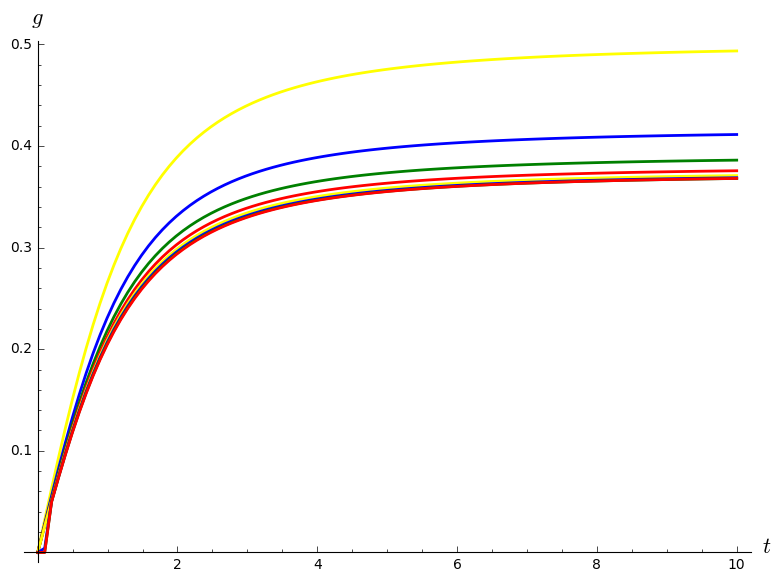
hence $\varphi_{g}:\mathbb{R}^{2}\to\mathbb{R}^{2}$ is the identity function and we recover the original spherical ensemble. The graphic of $g$ for some values of $d$ can be see in Figure 1.

Refer to caption — Figure 1. The function $g$ for different values of $d$ : from top to bottom, $d=2,3,4,5,6,7$ and $8$ .

Theorem 4.4.

Let $d\geq 1$ and let $N$ be of the form $N={d+L\choose d}$ . Then, $\mathfrak{X}_{*}^{(N)}$ is a homogeneous projection DPP in $\mathbb{S}^{2d}$ with kernel

K_{*}^{(N)}(p,q)=\frac{N}{Vol(\mathbb{S}^{2d})}\frac{\left(1+\left\langle z,w\right\rangle\right)^{L}}{(1+\|z\|^{2})^{\frac{L}{2}}(1+\|w\|^{2})^{\frac{L}{2}}}

where $z=\varphi_{g}^{-1}(\Pi_{d}(p)),\;w=\varphi_{g}^{-1}(\Pi_{d}(q))$ .

5. The expected Riesz s-energy of the generalized spherical ensemble

The Riesz $s$ –energy of a set on points $\omega_{N}=\{x_{1},\ldots,x_{N}\}$ on the sphere $\mathbb{S}^{d}$ with $s>0$ is

\mathcal{E}_{s}(\omega_{N})=\displaystyle\sum_{i\neq j}\frac{1}{\|x_{i}-x_{j}\|^{s}}

An interesting problem regarding this energy consists on looking for the minimal value that the energy can reach for a set of $N$ points on a sphere of dimension $d$ . The asymptotic behavior (for $N\to\infty$ ) has been extensively studied. In [9, 12] it was proved that for $d>2$ and $0<s<d$ there exist constants $c>C>0$ (depending only on $d$ and $s$ ) such that

(6)

\min_{\omega_{N}}\left(\mathcal{E}_{s}(\omega_{N})\right)\leq V_{s}(\mathbb{S}^{d})N^{2}-CN^{1+\frac{s}{d}}+o(N^{1+\frac{s}{d}}),

\min_{\omega_{N}}\left(\mathcal{E}_{s}(\omega_{N})\right)\geq V_{s}(\mathbb{S}^{d})N^{2}-cN^{1+\frac{s}{d}}+o(N^{1+\frac{s}{d}}),

where $V_{s}(\mathbb{S}^{d})$ is the continuous s-energy for the normalized Lebesgue measure,

V_{s}(\mathbb{S}^{d})=\frac{1}{Vol(\mathbb{S}^{d})^{2}}\displaystyle\int_{p,q\in\mathbb{S}^{d}}\frac{1}{\|p-q\|^{s}}dpdq=2^{d-s-1}\frac{\Gamma\left(\frac{d+1}{2}\right)\Gamma\left(\frac{d-s}{2}\right)}{\sqrt{\pi}\Gamma\left(d-\frac{s}{2}\right)}.

Finding precise bounds for the constants in (6) is an important open problem and has been addressed by several authors, see [7, 5] for some very precise conjectures and [8] for a survey paper. A strategy for the upper bound is to take collections of random points in $\mathbb{S}^{d}$ coming from DPPs and then compute the expected value of the energy (which is of course greater than or equal to the minimum possible value). This was done in the case of the harmonic ensemble, obtaining the best bounds known until date for general $s$ and even $d$ . Namely,

(7)

\begin{split}\min_{\omega_{N}}\left(\mathcal{E}_{s}(\omega_{N})\right)\leq&V_{s}(\mathbb{S}^{d})N^{2}-\frac{2^{s-\frac{s}{d}}V_{s}(\mathbb{S}^{d})d\,\Gamma\left(1+\frac{d}{2}\right)\Gamma\left(\frac{1+s}{2}\right)\Gamma\left(d-\frac{s}{2}\right)}{\sqrt{\pi}\Gamma\left(1+\frac{s}{2}\right)\Gamma\left(1+\frac{s+d}{2}\right)\left(d!\right)^{1-\frac{s}{d}}}N^{1+\frac{s}{d}}\\ &+o(N^{1+\frac{s}{d}}).\end{split}

In the case of odd-dimensional spheres, the best bound is obtained from a point process that is not determinantal but follows from a DPP (the projective ensemble described above), see [3]. For example the expression for the $2$ -energy that one gets with this process is:

(8)

\begin{split}&\min_{\omega_{N}}\left(\mathcal{E}_{2}(\omega_{N})\right)\leq V_{2}(\mathbb{S}^{d})N^{2}-\\ &\qquad\frac{3^{1-\frac{2}{2d+1}}(2d-1)^{1-\frac{2}{2d+1}}(2d+1)\Gamma\left(d-\frac{1}{2}\right)^{2-\frac{2}{2d+1}}}{2^{4-\frac{2}{2d+1}}(d!)^{2-\frac{4}{2d+1}}}N^{1+\frac{2}{d}}+o(N^{1+\frac{2}{d}}).\end{split}

For the generalized spherical ensemble, our result can be written as follows.

Theorem 5.1.

Let $N$ be of the form $N={d+L\choose d}$ , $d\geq 1$ and $0<s<2d$ , then

\text{\rm E}_{x\sim\mathfrak{X}_{*}^{(N)}}\left[\mathcal{E}_{s}(\omega_{N})\right]\leq V_{s}(\mathbb{S}^{2d})N^{2}\\ -\frac{Vol(\mathbb{S}^{2d-1})\left(\frac{(2d-s)\left(1-\frac{1}{d}\right)}{2e}\right)^{d-\frac{s}{2}}}{(2d-s)Vol(\mathbb{S}^{2d}))(d!)^{1-\frac{s}{2d}}}\left(1-\frac{e^{-1+\frac{1}{2d}}}{2\sqrt{1-\frac{1}{2d}}}\right)N^{1+\frac{s}{2d}}+o(N^{1+\frac{s}{2d}}).

If we compare our result with that from (7), we note that our bound is worst (see figure 2). Nevertheless, the points coming from this generalized spherical ensemble do respect the asymptotic of the minimal energy, getting the correct exponent $1+s/d$ for the second term in the expansion.

The technical version of Theorem 5.1 is a bound of the expected value of Riesz s-energy for points drawn from $\mathfrak{X}_{*}^{(N)}$ .

Theorem 5.2.

Let $d\geq 1$ and let $N$ be of the form $N={d+L\choose d}$ . Then, for $\tau>0$ such that $\tau<1-1/\sqrt{d}$ we have:

\text{\rm E}_{x\sim\mathfrak{X}_{*}^{(N)}}\left[\mathcal{E}_{s}(\omega_{N})\right]\leq N^{2}V_{s}(\mathbb{S}^{2d})-\frac{N^{2}Vol(\mathbb{S}^{2d-1})}{(2d-s)Vol(\mathbb{S}^{2d})}\times\\ \left(1-\frac{\tau^{2}}{4}\right)^{d-1}\tau^{2d-s}\left(1-\tau^{2}\frac{(1+\tau^{2})^{2}}{1-\left(\frac{1}{\sqrt{d}}+\tau\right)^{2}}\right)^{L}\left(1-\frac{e^{-1+\frac{1}{2d}}}{2\sqrt{1-\frac{1}{2d}}}\right)

Theorem 5.1 will follow from Theorem 5.2 by choosing the optimal value for $\tau$ .

6. An inequality regarding the incomplete Beta function

In order to prove Theorem 5.1 we will need an inequality regarding Euler’s incomplete Beta function. This inequality, which is sharp and might be of independent interest, is stated and proved in this section. Let us recall the definition of Euler’s incomplete Beta function (and its regularized version):

(9)

\mathrm{B}_{x}(a,b)=\int_{0}^{x}t^{a-1}(1-t)^{b-1}\,dt,\quad\mathrm{I}_{x}(a,b)=\frac{\mathrm{B}_{x}(a,b)}{\mathrm{B}(a,b)},

which satisfies $\mathrm{I}_{1}(a,b)=1$ .

Theorem 6.1.

Let $d\geq 1$ and $s\in[0,1]$ . Then,

d\mathrm{B}_{s}(d,d)\sqrt{1-(\mathrm{I}_{s}(d,d))^{\frac{1}{d}}}\geq s^{d}(1-s)^{d},

with an equality if and only if $s=0,1$ .

Before proving Theorem 6.1 we state a technical lemma:

Lemma 6.2.

The function

f(s)=dB_{s}(d,d)+s^{d}(1-s)^{d}\left(d-2ds-\sqrt{d^{2}(1-2s)^{2}+1+2d}\right)

satisfies $f(s)\geq 0$ for $s\in(0,1)$ .

Proof.

We note that $f(0)=0$ and we compute $f^{\prime}(s)=ds^{d-1}(1-s)^{d-1}h(s)$ where

h(s)=1+(1-2s)\left(d-2ds-\sqrt{d^{2}(1-2s)^{2}+1+2d}\right)+\\ s(1-s)\left(-2+\frac{2d(1-2s)}{\sqrt{d^{2}(1-2s)^{2}+1+2d}}\right).

It suffices to prove that $h(s)\geq 0$ for $s\in(0,1)$ . Denoting $u(s)=d^{2}(1-2s)^{2}+1+2d$ we have

h(s)=1+d(1-2s)^{2}-2s(1-s)+(1-2s)\sqrt{u(s)}\left(\frac{2ds(1-s)-u(s)}{u(s)}\right).

Since $2ds(1-s)<u(s)$ for all $s\in(0,1)$ we conclude that if $s>1/2$ then all the terms in $h(s)$ are positive and $h(s)\geq 0$ . It remains to prove $h(s)\geq 0$ for $s\in(0,1/2)$ . Then, the claim is equivalent to

\left(1+d(1-2s)^{2}-2s(1-s)\right)^{2}\geq(1-2s)^{2}u(s)\left(\frac{2ds(1-s)-u(s)}{u(s)}\right)^{2},

that is

u(s)\left(1+d(1-2s)^{2}-2s(1-s)\right)^{2}-(1-2s)^{2}(2ds(1-s)-u(s))^{2}\geq 0.

Expanding the terms, the last expression equals

s^{2}(1-s)^{2}(4+8d)\geq 0,

which trivially holds, thus proving the lemma. ∎

6.1. Proof of Theorem 6.1

Some elementary algebraic manipulations show that the inequality of the theorem is equivalent to:

f(s)\geq\frac{1}{B(d,d)},\quad f(s)=Q(s)\,(1-Q(s)^{2}A(s))^{d}

where $Q(s)=B_{s}(d,d)^{-1}$ and $A(s)=s^{2d}(1-s)^{2d}/d^{2}$ . Now, note that

f(1)=\frac{1}{B(d,d)},

and hence it suffices to show that $f$ is a non–increasing function. We compute the derivative

f^{\prime}(s)=(1-Q(s)^{2}A(s))^{d-1}\left(Q^{\prime}(s)-(1+2d)Q^{\prime}(s)Q(s)^{2}A(s)-dQ(s)^{3}A^{\prime}(s)\right),

and hence it suffices to see that

Q^{\prime}(s)-(1+2d)Q^{\prime}(s)Q(s)^{2}A(s)-dQ(s)^{3}A^{\prime}(s)\leq 0,\quad s\in(0,1),

or equivalently we just have to see that

dA^{\prime}(s)B_{s}(d,d)+s^{d-1}(1-s)^{d-1}(B_{s}(d,d)^{2}-(1+2d)A(s))\geq 0,\quad s\in(0,1).

Computing the derivative $A^{\prime}(s)$ and simplifying, this last inequality is equivalent to

B_{s}(d,d)^{2}+2s^{d}(1-s)^{d}(1-2s)B_{s}(d,d)-\frac{1+2d}{d^{2}}s^{2d}(1-s)^{2d}\geq 0,

and hence also to

\left(B_{s}(d,d)+s^{d}(1-s)^{d}(1-2s)\right)^{2}\geq s^{2d}(1-s)^{2d}(1-2s)^{2}+\frac{1+2d}{d^{2}}s^{2d}(1-s)^{2d}\\ =s^{2d}(1-s)^{2d}\left((1-2s)^{2}+\frac{1+2d}{d^{2}}\right),

which follows from Lemma 6.2 after taking square roots. Theorem 6.1 now follows.

7. Proofs of the main results

In order to prove the results presented in this paper, we will define two more functions.

Definition 7.1.

Let $\theta:\mathbb{C}^{d}\to\mathbb{S}^{2d}$ be the mapping defined by $\theta(x)=\frac{(x,1)}{\|(x,1)\|}$ . We denote by $\phi(x)=(\theta\circ\varphi^{-1}\circ\Pi)(x)$ , where $\varphi^{-1}$ and $\Pi$ are defined in Definition 4.1.

Note that $\phi$ maps $\mathbb{S}^{2d}$ into its upper half.

7.1. Derivatives of the stereographic projection and other mappings

In this section we state an elementary lemma with the computation of the derivative of the stereographic projection and other mappings.

Let $\mathbf{n}=(0,\ldots,0,1)\in\mathbb{S}^{2d}$ be the north pole and let $p\in\mathbb{S}^{2d}$ , $p\neq\pm\mathbf{n}$ . It is useful to consider an orthonormal basis $\{\dot{p}^{1},\ldots,\dot{p}^{2d-1},\dot{p}^{2d}\}$ of $p^{\perp}$ such that $\dot{p}^{i}\perp\mathbf{n}$ for $1\leq i\leq 2d-1$ and

\dot{p}^{2d}=\frac{\mathbf{n}-p_{2d+1}p}{\sqrt{1-p_{2d+1}^{2}}}.

Lemma 7.2.

Let $\Pi$ be the stereographic projection (4), let $\varphi_{g}$ be as defined in Definition 4.1 and let $\theta$ be as defined in Definition 7.1. Then,

\begin{split}D\Pi(p)\dot{p}=&\left[\frac{\dot{p_{1}}}{1-p_{2d+1}}+\frac{p_{1}\dot{p}_{2d+1}}{(1-p_{2d+1})^{2}},\ldots,\frac{\dot{p_{2d}}}{1-p_{2d+1}}+\frac{p_{2d}\dot{p}_{2d+1}}{(1-p_{2d+1})^{2}}\right],\\ D\varphi_{g}^{-1}(y)\dot{y}=&(g^{-1})^{\prime}(\|y\|)\frac{y\Re(\left\langle y,\dot{y}\right\rangle)}{\|y\|^{2}}+g^{-1}(\|y\|)\frac{\dot{y}\|y\|-y\frac{\Re(\left\langle y,\dot{y}\right\rangle)}{\|y\|}}{\|y\|^{2}},\\ D\theta(x)\dot{x}=&\frac{(\dot{x},0)\|(x,1)\|-(x,1)\frac{\Re(\left\langle(x,1),(\dot{x},0)\right\rangle)}{\|(x,1)\|}}{\|(x,1)\|^{2}}.\end{split}

Here we are denoting by $\Re(z)$ the real part of a complex number $z$ .

Proof.

This computation is an exercise left to the reader. It is convenient to consider the basis described before the lemma.

$\square$

Corollary 7.3.

The Jacobian determinants of $\Pi$ and $\varphi_{g}^{-1}$ satisfy:

	$\displaystyle\mathrm{Jac}\Pi(p)=$	$\displaystyle\frac{1}{(1-p_{2d+1})^{2d}}=\left(\frac{1+\\|\Pi(p)\\|^{2}}{2}\right)^{2d},$
	$\displaystyle\mathrm{Jac}\varphi_{g}^{-1}(y)=$	$\displaystyle(g^{-1})^{\prime}(\\|y\\|)\left(\frac{g^{-1}(\\|y\\|)}{\\|y\\|}\right)^{2d-1}.$

Proof.

Let $p\neq\pm\mathbf{n}$ and let $\dot{p}^{1},\ldots,\dot{p}^{2d-1},\dot{p}^{2d}$ be the basis described at the beginning of this section. Then, it is clear from Lemma 7.2 that $D\Pi(p)$ preserves the orthogonality of the basis and a little algebra shows that it is an homothetic transformation with ratio $(1-p_{2d+1})^{-1}$ , hence

\mathrm{Jac}\Pi(p)=\frac{1}{(1-p_{2d+1})^{2d}}.

And noting that

\|\Pi(p)\|^{2}=\frac{1+p_{2d+1}}{1-p_{2d+1}}\Rightarrow p_{2d+1}=\frac{\|\Pi(p)\|^{2}-1}{\|\Pi(p)\|^{2}+1},

the first claim of the corollary follows.

For the second Jacobian, given $y\in\mathbb{C}^{d}\equiv\mathbb{R}^{2d}$ we consider an orthonormal basis $\dot{v}^{1},\ldots,\dot{v}^{2d}$ whose last vector is $y/\|y\|$ . Then, $D\varphi_{g}^{-1}$ preserves the orthogonality of this basis and hence we have

\mathrm{Jac}\varphi_{g}^{-1}(y)=\|D\varphi_{g}^{-1}(y)(y/\|y\|)\|\cdot\prod_{i=1}^{2d-1}\|D\varphi_{g}^{-1}(y)\dot{v}^{i}\|,

which from Lemma 7.2 equals

(g^{-1})^{\prime}(\|y\|)\cdot\prod_{i=1}^{2d-1}\frac{g^{-1}(\|y\|)}{\|y\|},

and the corollary follows.

7.2. Proof of Proposition 4.2

The push-forward of a projection DPP is a DPP, see [3, Proposition 2.5] for a proof. So $\mathfrak{X}_{*}^{(N,d,g)}$ is a DPP in $\mathbb{S}^{2d}$ , and from the same proposition and equation (3), we know that its associated kernel is

(10)

K_{*}^{(N,d,g)}(p,q)=\frac{Nd!}{{\pi}^{d}}\frac{(1+\left\langle z,w\right\rangle)^{L}\sqrt{|\text{\rm Jac}(\varphi_{g}^{-1}\circ\Pi)(z)\text{\rm Jac}(\varphi_{g}^{-1}\circ\Pi)(z)|}}{(1+\|z\|^{2})^{\frac{d+L+1}{2}}(1+\|w\|^{2})^{\frac{d+L+1}{2}}},

where $z=\varphi_{g}^{-1}(\Pi(p)),\;w=\varphi_{g}^{-1}(\Pi(q))$ . Now, from the chain rule,

\mathrm{Jac}(\varphi_{g}^{-1}\circ\Pi)(p)=\mathrm{Jac}(\varphi_{g}^{-1})(\Pi(p))\mathrm{Jac}\Pi(p).

From Corollary 7.3, this last equals

(g^{-1})^{\prime}(\|\Pi(p)\|)\left(\frac{g^{-1}(\|\Pi(p)\|)}{\|\Pi(p)\|}\right)^{2d-1}\left(\frac{1+\|\Pi(p)\|^{2}}{2}\right)^{2d}.

Now, $\|\Pi(p)\|=\|\varphi_{g}(z)\|=g(\|z\|)$ and thus we have:

\mathrm{Jac}(\phi^{-1})(p)=(g^{-1})^{\prime}(g(\|z\|))\left(\frac{\|z\|}{g(\|z\|)}\right)^{2d-1}\left(\frac{1+g(\|z\|)^{2}}{2}\right)^{2d},

namely:

(11)

\mathrm{Jac}(\phi^{-1})(p)=\frac{1}{g^{\prime}(\|z\|)}\left(\frac{\|z\|}{g(\|z\|)}\right)^{2d-1}\left(\frac{1+g(\|z\|)^{2}}{2}\right)^{2d},

and the same holds changing $p$ to $q$ and $z$ to $w$ . Putting together (10) and (11) we get Proposition 4.2.

7.3. Proof of Proposition 4.3

During this proof, we denote by $K_{*}$ the kernel $K_{*}^{(N,d,g)}$ . From Proposition 4.2:

\begin{split}K_{*}(p,p)=\frac{Nd!}{\pi^{d}2^{2d}}\frac{(g(\|z\|)^{2}+1)^{2d}\|z\|^{2d-1}}{g^{\prime}(\|z\|)g(\|z\|)^{2d-1}(1+\|z\|^{2})^{d+1}}.\\ \end{split}

From Proposition 2.3, if the DPP associated to $K_{*}$ is homogeneus then $K_{*}(p,p)=N/Vol(\mathbb{S}^{2d})$ for all $p\in\mathbb{S}^{2d}$ . Thus, in order for the process to be homogeneus one must have:

\frac{Nd!}{\pi^{d}2^{2d}}\frac{(g(t)^{2}+1)^{2d}t^{2d-1}}{g^{\prime}(t)g(t)^{2d-1}(1+t^{2})^{d+1}}=\frac{N}{Vol(\mathbb{S}^{2d})}=\frac{N\Gamma\left(d+\frac{1}{2}\right)}{2\pi^{d+\frac{1}{2}}},\quad t\in(0,\infty),

namely,

(12)

\frac{g^{\prime}(t)g(t)^{2d-1}}{(g(t)^{2}+1)^{2d}}=\frac{\sqrt{\pi}d!}{2^{2d-1}\Gamma\left(d+\frac{1}{2}\right)}\frac{t^{2d-1}}{(1+t^{2})^{d+1}}=dB(d,d)\frac{t^{2d-1}}{(1+t^{2})^{d+1}},

where we have used Legendre’s duplication formula for the Gamma function (see [1, Formula 5.5.5]),

(13)

\Gamma(z)\;\Gamma\left(z+\frac{1}{2}\right)=2^{1-2z}\;\sqrt{\pi}\;\Gamma(2z)\,.\!

Now we integrate (12) in both sides. On one hand,

\begin{split}\displaystyle\int dB(d,d)\frac{t^{2d-1}}{(1+t^{2})^{d+1}}dt=\frac{B(d,d)}{2}\frac{t^{2d}}{(1+t^{2})^{d}}\\ \end{split}.

On the other hand,

\begin{split}&\displaystyle\int\frac{g^{2d-1}}{(g^{2}+1)^{2d}}dg=\frac{1}{2}\left[B(d,d)-\mathrm{B}_{\frac{1}{1+g^{2}}}(d,d)\right]\end{split},

where $\mathrm{B}_{x}$ denotes Euler’s incomplete Beta function (see equation (9) for a definition). We thus have (using the regularized incomplete Beta function):

1-\mathrm{I}_{\frac{1}{1+g^{2}}}(d,d)=\frac{t^{2d}}{(1+t^{2})^{d}},

where the chosen integration constant is the unique with the property that $g(0)=0$ . Recall that $\mathop{\mathrm{I}_{x}\/}\nolimits\!\left(a,b\right)=1-\mathop{\mathrm{I}_{1-x}\/}\nolimits\!\left(b,a\right)$ (see for example [1]). Hence, the function $g$ we are looking for must satisfy:

\mathrm{I}_{\frac{g^{2}}{1+g^{2}}}(d,d)=\left(\frac{t^{2}}{1+t^{2}}\right)^{d}.

Note that $g$ is well–defined since the regularized Beta function is bijective in the range $[0,1]$ and for all $t\in(0,\infty)$ , $0<\frac{t^{2}}{1+t^{2}}<1$ .

We also check that $g$ satisfies the claimed properties:

•

$\boldsymbol{g}$ is an increasing function: $g$ satisfies the differential equation (12) and thus the derivative is positive.
•

$\boldsymbol{g(0)=0}$ since we have chosen the correct integration constant.
•

$\boldsymbol{\lim\limits_{t\rightarrow\infty}g(t)=\infty}$ : $\lim\limits_{t\rightarrow\infty}\mathrm{I}_{\frac{g^{2}}{1+g^{2}}}(d,d)=\lim\limits_{t\rightarrow\infty}\left(\frac{t^{2}}{1+t^{2}}\right)^{d}=1$ .

Now if $\lim\limits_{t\rightarrow\infty}\mathrm{I}_{\frac{g^{2}}{1+g^{2}}}(d,d)=1\Rightarrow\lim\limits_{t\rightarrow\infty}\frac{g^{2}}{1+g^{2}}=1\Rightarrow\lim\limits_{t\rightarrow\infty}g=\pm\infty$ . Since $g$ is increasing and $g(0)=0$ , the only possible solution is $\lim\limits_{t\rightarrow\infty}g=\infty.$
•

$\boldsymbol{g}$ is $\boldsymbol{\mathcal{C}^{\infty}}$ : since $t\to\left(\frac{t^{2}}{1+t^{2}}\right)^{d}$ is $\mathcal{C}^{\infty}$ and so is the inverse regularized incomplete Beta function, we conclude that $t\to s(t)=\frac{g(t)^{2}}{1+g(t)^{2}}$ is $\mathcal{C}^{\infty}$ . Then we can solve $g=\sqrt{\frac{s}{1-s}}$ , so in the interval $s\in(0,1)$ , $g$ is a composition of $\mathcal{C}^{\infty}$ functions whose denominator does not vanish and thereby is $\mathcal{C}^{\infty}$ .

$\square$

7.4. Proof of Theorem 4.4

We only have to replace the expresion for $g^{\prime}(t)$ given in equation (12) to compute $R(t)$ from Proposition 4.2:

R(t)=\frac{1}{\sqrt{d\mathrm{B}(d,d)}(1+t^{2})^{L/2}}.

We then have:

K_{*}^{(N)}(p,q)=\frac{Nd!}{\pi^{d}2^{2d}d\mathrm{B}(d,d)}\frac{\left(1+\left\langle z,w\right\rangle\right)^{L}}{(1+\|z\|^{2})^{\frac{L}{2}}(1+\|w\|^{2})^{\frac{L}{2}}}.

The expression for the constant $N/Vol(\mathbb{S}^{2d})$ follows using (13) and (1).

7.5. Proof of Theorem 5.2

It is well known (see for example [10, Formula 1.2.2.]) that the expected value of the Riesz energy of a set of $N$ points coming from $\mathfrak{X}_{*}^{(N)}$ satisfies:

\begin{split}\text{\rm E}_{x\sim\mathfrak{X}_{*}^{(N)}}\left[\mathcal{E}_{s}(x_{1},\ldots,x_{N})\right]&=\displaystyle\int_{\mathbb{S}^{2d}\times\mathbb{S}^{2d}}\frac{K_{*}^{(N)}(p,p)^{2}-|K_{*}^{(N)}(p,q)|^{2}}{\|p-q\|^{s}}dpdq\\ &=\frac{N^{2}}{Vol(\mathbb{S}^{2d})^{2}}\displaystyle\int_{\mathbb{S}^{2d}\times\mathbb{S}^{2d}}\frac{1-\left(\frac{|K_{*}^{(N)}(p,q)|}{K_{*}^{(N)}(p,p)}\right)^{2}}{\|p-q\|^{s}}dpdq\\ &=N^{2}V_{s}(\mathbb{S}^{2d})-\frac{N^{2}}{Vol(\mathbb{S}^{2d})^{2}}\displaystyle\int_{\mathbb{S}^{2d}\times\mathbb{S}^{2d}}\frac{\left(\frac{|K_{*}^{(N)}(p,q)|}{K_{*}^{(N)}(p,p)}\right)^{2}}{\|p-q\|^{s}}dpdq.\end{split}

Bounding the integral in the last term is a non–trivial task. We will do it in several steps.

Proposition 7.4.

Let $p,q$ be points of $\mathbb{S}^{2d}$ , then

\left(\frac{|K_{*}^{(N)}(p,q)|}{K_{*}^{(N)}(p,p)}\right)^{2}\geq\max\left\{(1-\|\phi(p)-\phi(q)\|^{2})^{L},0\right\}

where $\phi$ was defined in Definition 7.1.

Proof.

It is obvious that $\left(\frac{|K_{*}^{(N)}(p,q)|}{K_{*}^{(N)}(p,p)}\right)^{2}\geq 0$ . We will use the fact that for every unit vectors $x,y\in\mathbb{C}^{a}$ , we have

|\left\langle x,y\right\rangle|^{2}\geq\Re(\langle x,y\rangle)^{2}=\left(1-\frac{\|x-y\|^{2}}{2}\right)^{2}\geq 1-\|x-y\|^{2}.

Then,

\begin{split}\left(\frac{|K_{*}^{(N)}(p,q)|}{K_{*}^{(N)}(p,p)}\right)^{2}=&\left(\frac{|1+\left\langle z,w\right\rangle|^{2}}{(1+\|z\|^{2})(1+\|w\|^{2})}\right)^{L}=\left|\frac{\left\langle(z,1),(w,1)\right\rangle}{\sqrt{1+\|z\|^{2}}\sqrt{1+\|w\|^{2}}}\right|^{2L}=\\ &=\left|\left\langle\frac{(z,1)}{\|(z,1)\|},\frac{(w,1)}{\|(w,1)\|}\right\rangle\right|^{2L}\geq\left(1-\left\|\frac{(z,1)}{\|(z,1)\|}-\frac{(w,1)}{\|(w,1)\|}\right\|^{2}\right)^{L}=\\ &=\left(1-\left\|\frac{(\varphi^{-1}(\Pi(p)),1)}{\|(\varphi^{-1}(\Pi(p)),1)\|}-\frac{(\varphi^{-1}(\Pi(q)),1)}{\|(\varphi^{-1}(\Pi(q)),1)\|}\right\|^{2}\right)^{L}=\\ &=(1-\|\phi(p)-\phi(q)\|^{2})^{L}.\end{split}

$\square$

Lemma 7.5.

Let $p,q\in\mathbb{S}^{2d}$ , then the following inequality holds.

\|\phi(p)-\phi(q)\|\leq\left(\|p-q\|+\|p-q\|^{3}\right)\sup\|D\phi(x)\|,

where the supremum is taken for $x$ in the geodesic from $p$ to $q$ .

Proof.

Given two points $p,q\in\mathbb{S}^{2d}$ , let $\alpha=d_{\mathbb{S}^{2d}}(p,q)$ where $d_{\mathbb{S}^{2d}}$ is the distance in the sphere, and let $\gamma$ be the geodesic segment from $p$ to $q$ . Then we have

	$\displaystyle\\|\phi(p)-\phi(q)\\|=$	$\displaystyle\\|\phi(\gamma(0))-\phi(\gamma(\alpha))\\|\leq\left\\|\displaystyle\int_{0}^{\alpha}D\phi(\gamma(t))\dot{\gamma}(t)dt\right\\|$
	$\displaystyle\leq$	$\displaystyle\displaystyle\int_{0}^{\alpha}\left\\|D\phi(\gamma(t))\dot{\gamma}(t)\right\\|dt\leq\alpha\sup\\|D\phi(x)\\|.$

where $x$ lies on the geodesic from $p$ to $q$ . We now note that

\alpha=d_{\mathbb{S}^{2d}}(p,q)=2\arcsin\left(\frac{\|p-q\|}{2}\right)\leq\|p-q\|+\|p-q\|^{3},

the last since $2\arcsin(x/2)\leq x+x^{3}$ for $0\leq x\leq 2$ (a simple exercise left to the reader). The lemma follows.

$\square$

Proposition 7.6.

Let $\mathbf{n}=(0,\ldots,0,1)\in\mathbb{S}^{2d}$ be the north pole and let $p\in\mathbb{S}^{2d}$ , $p\neq\mathbf{n}$ . Let $\dot{p}^{1},\ldots,\dot{p}^{2d}$ be the orthonormal basis of $p^{\perp}$ defined in Section 7.1. Then, $D\phi(p)$ preserves the orthogonality of the basis and we have

\left\|D\phi(p)\dot{p}^{i}\right\|=\frac{g^{-1}\left(\sqrt{\frac{1+p_{2d+1}}{1-p_{2d+1}}}\right)}{\sqrt{1-p_{2d+1}^{2}}\sqrt{1+\left(g^{-1}\left(\sqrt{\frac{1+p_{2d+1}}{1-p_{2d+1}}}\right)\right)^{2}}},\quad 1\leq i\leq 2d-1,

and

\left\|D\phi(p)\dot{p}^{2d}\right\|=\frac{(g^{-1})^{\prime}\left(\sqrt{\frac{1+p_{2d+1}}{1-p_{2d+1}}}\right)}{\left(1+g^{-1}\left(\sqrt{\frac{1+p_{2d+1}}{1-p_{2d+1}}}\right)^{2}\right)(1-p_{2d+1})}.

In particular, $\|D\phi(p)\|$ is the supremum of these two quantities.

Proof.

We recall that $\phi(p)=(\theta\circ\varphi^{-1}\circ\Pi)(p)$ .

Using the chain rule,

D\phi(p)\dot{p}=D(\theta\circ\varphi^{-1}\circ\Pi)(p)\dot{p}=D\theta(\varphi^{-1}(\Pi(p)))D\varphi^{-1}(\Pi(p))D\Pi(p)\dot{p}.

From Lemma 7.2, after some algebra we get for $1\leq i\leq 2d-1$ :

D\theta(\varphi^{-1}(\Pi(p)))D\varphi^{-1}(\Pi(p))D\Pi(p)\dot{p}^{i}=\frac{g^{-1}\left(\sqrt{\frac{1+p_{2d+1}}{1-p_{2d+1}}}\right)}{\sqrt{1-p_{2d+1}^{2}}\sqrt{1+\left(g^{-1}\left(\sqrt{\frac{1+p_{2d+1}}{1-p_{2d+1}}}\right)\right)^{2}}}\dot{p}^{i},

while for $\dot{p}^{2d}$ we get

\begin{split}&D\theta(\varphi^{-1}(\Pi(p)))D\varphi^{-1}(\Pi(p))D\Pi(p)\frac{\mathbf{n}-p_{2d+1}p}{\sqrt{1-p_{2d+1}^{2}}}=\\ &\frac{(g^{-1})^{\prime}\left(\sqrt{\frac{1+p_{2d+1}}{1-p_{2d+1}}}\right)}{\sqrt{1-p_{2d+1}^{2}}(1-p_{2d+1})\sqrt{1+\left(g^{-1}\left(\sqrt{\frac{1+p_{2d+1}}{1-p_{2d+1}}}\right)\right)^{2}}^{3}}\left(\begin{array}[]{c}p_{1}\\ \ldots\\ p_{2d}\\ -g^{-1}\left(\sqrt{\frac{1+p_{2d+1}}{1-p_{2d+1}}}\right)\sqrt{1-p_{2d+1}^{2}}\end{array}\right)\end{split}

Both the preservation of the orthogonality of the basis through $D\phi(p)$ and the formulas for the norm of $D\phi(p)\dot{p}^{i}$ follow, and the proposition is proved.

$\square$

We need to compute the supremum among the two quantities of Proposition 7.6, which is a nontrivial task. Following the same notation we have:

Lemma 7.7.

Fix any $d\geq 1$ . The two following claims are equivalent:

(1)

For all $p=(p_{1},\ldots,p_{2d+1})\in\mathbb{S}^{2d}$ we have

$\left\|D\phi(p)\dot{p}^{i}\right\|\geq\left\|D\phi(p)\frac{\mathbf{n}-p_{2d+1}p}{\sqrt{1-p_{2d+1}^{2}}}\right\|.$

(Here, $\dot{p}^{i}$ , $1\leq i\leq 2d-1$ , are as in Proposition 7.6.)
(2)

For all $s\in(0,1)$ we have

$d\mathrm{B}_{s}(d,d)\sqrt{1-(\mathrm{I}_{s}(d,d))^{\frac{1}{d}}}\geq s^{d}(1-s)^{d}.$

Proof.

The claim is the result of a lengthy computation obtained by working on the expressions from Proposition 7.6 using the definition of $g$ given in Proposition 4.3, which can be written as:

(14)

g^{-1}(s)=\left(\frac{\mathrm{I}_{\frac{s^{2}}{1+s^{2}}}(d,d)^{1/d}}{1-\mathrm{I}_{\frac{s^{2}}{1+s^{2}}}(d,d)^{1/d}}\right)^{1/2}.

$\square$

From Lemma 7.7 and Theorem 6.1 we readily have:

Proposition 7.8.

For all $d\geq 1$ and all $p\in\mathbb{S}^{2d}$

\left\|D\phi(p)\dot{p}^{i}\right\|\geq\left\|D\phi(p)\frac{\mathbf{n}-p_{2d+1}p}{\sqrt{1-p_{2d+1}^{2}}}\right\|,

where $\dot{p}^{i}$ , $1\leq i\leq 2d-1$ , are as in Proposition 7.6.

Corollary 7.9.

Let $p,q\in\mathbb{S}^{2d}$ , $\|p-q\|\leq\tau$ and $p_{2d+1}<\epsilon$ where $0<\epsilon+\tau<1$ . Then, for every $x\in\mathbb{S}^{2d}$ in the geodesic segment from $p$ to $q$ we have

(15)

\left\|D\phi(x)\right\|\leq\frac{g^{-1}\left(\sqrt{\frac{1+(\tau+\epsilon)}{1-(\tau+\epsilon)}}\right)}{\sqrt{1-(\tau+\epsilon)^{2}}\sqrt{1+\left(g^{-1}\left(\sqrt{\frac{1+(\tau+\epsilon)}{1-(\tau+\epsilon)}}\right)\right)^{2}}}\leq\frac{1}{\sqrt{1-(\tau+\epsilon)^{2}}}=M_{\epsilon,\tau}.

Proof.

The second inequality is trivial. For the first one, note that from propositions 7.6 and 7.8, for $x$ as in the hypotheses we have

\|D\phi(x)\dot{x}\|\leq\frac{g^{-1}\left(\sqrt{\frac{1+x_{2d+1}}{1-x_{2d+1}}}\right)}{\sqrt{1-x_{2d+1}^{2}}\sqrt{1+\left(g^{-1}\left(\sqrt{\frac{1+x_{2d+1}}{1-x_{2d+1}}}\right)\right)^{2}}}\stackrel{{\scriptstyle\eqref{eq:otra}}}{{=}}\sqrt{\frac{\mathrm{I}_{\frac{1+x_{2d+1}}{2}}^{1/d}}{1-x_{2d+1}^{2}}}

It is clear that this is an increasing function of $x_{2d+1}$ . The claim of the proposition follows noting that $p_{2d+1}\leq\epsilon$ and $\|p-q\|\leq\tau$ implies $|x_{2d-1}-p_{2d+1}|\leq\tau$ and hence $x_{2d+1}\leq\tau+\epsilon$ .

$\square$

Proposition 7.10.

Let $\epsilon,\tau\in\left(0,1\right)$ with $\epsilon+\tau<1$ . Then for all $p,q\in\mathbb{S}^{2d}$ we have

\displaystyle\int_{p,q\in\mathbb{S}^{2d}}\frac{\left(\frac{|K_{*}^{(N)}(p,q)|}{K_{*}^{(N)}(p,p)}\right)^{2}}{\|p-q\|^{s}}dpdq\geq\\ \frac{W(\epsilon)Vol(\mathbb{S}^{2d-1})}{(2d-s)}\left(1-\frac{\tau^{2}}{4}\right)^{d-1}\tau^{2d-s}\left(1-\tau^{2}\frac{(1+\tau^{2})^{2}}{1-(\epsilon+\tau)^{2}}\right)^{L}

where $W(\epsilon)$ is the volume of the set of $p\in\mathbb{S}^{2d}$ such that $p_{2d+1}\leq\epsilon$ .

In order to prove Proposition 7.10, we present Lemma 7.11 (that follows from the change of variables formula applied to the projection from the cylinder to the sphere).

Lemma 7.11.

If $f:\mathbb{S}^{m}\to\mathbb{R}$ satisfies $f(q)=g(\langle p,q\rangle)$ , for some $p\in\mathbb{S}^{m}$ and some $g:\left[-1,1\right]\longrightarrow\mathbb{R}$ , then

\displaystyle\int_{p\in\mathbb{S}^{m}}f(p)dp=Vol(\mathbb{S}^{m-1})\displaystyle\int_{-1}^{1}g(t)(1-t^{2})^{\frac{m}{2}-1},

assuming that $f$ is integrable or $f$ is measurable and non–negative.

Proof (Proof of Proposition 7.10).

From lemmas 7.4 and 7.5 and Corollary 7.9, $\tau,\epsilon>0$ and $0<\tau+\epsilon<1$ we have:

\displaystyle\int_{\mathbb{S}^{2d}\times\mathbb{S}^{2d}}\frac{\left(\frac{|K_{*}^{(N)}(p,q)|}{K_{*}^{(N)}(p,p)}\right)^{2}}{\|p-q\|^{s}}dpdq\geq\displaystyle\int_{\|p-q\|\leq\tau,p_{2d+1}\leq\epsilon}\frac{\left(\frac{|K_{*}^{(N)}(p,q)|}{K_{*}^{(N)}(p,p)}\right)^{2}}{\|p-q\|^{s}}dpdq\geq\\ \displaystyle\int_{\|p-q\|\leq\tau,p_{2d+1}\leq\epsilon}\frac{\left(1-\frac{(1+\tau^{2})^{2}\|p-q\|^{2}}{1-(\epsilon+\tau)^{2}}\right)^{L}}{\|p-q\|^{s}}dpdq.\\

We apply Fubini’s theorem and Lemma 7.11, transforming the last integral into:

\begin{split}&\displaystyle\int_{p_{2d+1}\leq\epsilon}\left[\displaystyle\int_{\|p-q\|\leq\tau}\frac{\left(1-\frac{(1+\tau^{2})^{2}\|p-q\|^{2}}{1-(\epsilon+\tau)^{2}}\right)^{L}}{\|p-q\|^{s}}dq\right]dp=\\ \end{split}

\begin{split}&=\displaystyle\int_{p_{2d+1}\leq\epsilon}\left[\displaystyle\int_{\sqrt{2-2\langle p,q\rangle}\leq\tau}\frac{\left(1-\frac{(1+\tau^{2})^{2}}{1-(\epsilon+\tau)^{2}}(2-2\langle p,q\rangle)\right)^{L}}{\sqrt{2-2\langle p,q\rangle}^{\,s}}dq\right]dp=\\ \end{split}

(16)

\begin{split}&=Vol(\mathbb{S}^{2d-1})\displaystyle\int_{1-\frac{\tau^{2}}{2}}^{1}\frac{\left(1-\frac{(1+\tau^{2})^{2}}{1-(\epsilon+\tau)^{2}}(2-2t)\right)^{L}}{\sqrt{2-2t}^{\,s}}(1-t^{2})^{d-1}dt\displaystyle\int_{p_{2d+1}\leq\epsilon}dp.\end{split}

Then, (16) equals:

\frac{W(\epsilon)Vol(\mathbb{S}^{2d-1})}{2^{\frac{s}{2}}}\displaystyle\int_{1-\frac{\tau^{2}}{2}}^{1}\frac{\left(1-\frac{(1+\tau^{2})^{2}}{1-(\epsilon+\tau)^{2}}(2-2t)\right)^{L}}{\sqrt{1-t}^{s}}(1-t^{2})^{d-1}dt.

where $W(\epsilon)$ is the volume of the set of points of $\mathbb{S}^{2d}$ such that their last coordinate is less or equal to $\epsilon$ . With the change of variables $u=1-t$ and using $1-t^{2}=(1-t)(1+t)$ we have proved that:

(17)

\displaystyle\int_{\mathbb{S}^{2d}\times\mathbb{S}^{2d}}\frac{\left(\frac{|K_{*}^{(n)}(p,q)|}{K_{*}^{(n)}(p,p)}\right)^{2}}{\|p-q\|^{s}}dpdq\geq\\ \frac{W(\epsilon)Vol(\mathbb{S}^{2d-1})}{2^{\frac{s}{2}}}\left(2-\frac{\tau^{2}}{2}\right)^{d-1}\displaystyle\int_{0}^{\frac{\tau^{2}}{2}}\left(1-2\frac{(1+\tau^{2})^{2}}{1-(\epsilon+\tau)^{2}}u\right)^{L}u^{d-1-\frac{s}{2}}du.

Since $u\leq\frac{\tau^{2}}{2}$ , $\left(1-2\frac{(1+\tau^{2})^{2}}{1-(\epsilon+\tau)^{2}}u\right)^{L}\geq\left(1-\tau^{2}\frac{(1+\tau^{2})^{2}}{1-(\epsilon+\tau)^{2}}\right)^{L}$ and so

(18)

\displaystyle\int_{\mathbb{S}^{2d}\times\mathbb{S}^{2d}}\frac{\left(\frac{|K_{*}^{(n)}(p,q)|}{K_{*}^{(n)}(p,p)}\right)^{2}}{\|p-q\|^{s}}dpdq\geq\\ \frac{W(\epsilon)Vol(\mathbb{S}^{2d-1})}{2^{\frac{s}{2}}}\left(2-\frac{\tau^{2}}{2}\right)^{d-1}\left(1-\tau^{2}\frac{(1+\tau^{2})^{2}}{1-(\epsilon+\tau)^{2}}\right)^{L}\displaystyle\int_{0}^{\frac{\tau^{2}}{2}}u^{d-1-\frac{s}{2}}du.

We then have proved the following lower bound for the integral in the proposition:

\frac{W(\epsilon)Vol(\mathbb{S}^{2d-1})}{(2d-s)}\left(1-\frac{\tau^{2}}{4}\right)^{d-1}\tau^{2d-s}\left(1-\tau^{2}\frac{(1+\tau^{2})^{2}}{1-(\epsilon+\tau)^{2}}\right)^{L}.

The proof is now complete.

$\square$

7.5.1. Proof of Theorem 5.2

First we are going to give a bound for $W(\epsilon)$ .

Proposition 7.12.

Let $r>0$ and let $\vartheta\left(\frac{\pi}{2}+r\right)$ be the volume of the spherical cap of radius $\frac{\pi}{2}+r$ in $\mathbb{S}^{n+1}$ , then

\vartheta\left(\frac{\pi}{2}+r\right)\geq Vol(\mathbb{S}^{n+1})\left(1-\frac{e^{\frac{-r^{2}n}{2}}}{2}\sqrt{1+\frac{1}{n}}\right)

Proof.

As in [14, Corollary 2.2] we consider the normalized measure of $\vartheta\left(\frac{\pi}{2}+r\right)$ ,

\frac{\vartheta\left(\frac{\pi}{2}+r\right)}{Vol(\mathbb{S}^{n+1})}=\frac{\int_{\frac{-\pi}{2}}^{r}\cos^{n}\theta d\theta}{\int_{\frac{-\pi}{2}}^{\frac{\pi}{2}}\cos^{n}\theta d\theta}

The same result shows that

1-\frac{\vartheta\left(\frac{\pi}{2}+r\right)}{Vol(\mathbb{S}^{n+1})}\leq\frac{e^{\frac{-r^{2}n}{2}}\sqrt{\frac{\pi}{2}}}{2\sqrt{n}I_{n}},

where $I_{n}=\int_{0}^{\frac{\pi}{2}}\cos^{n}\theta d\theta=\frac{\sqrt{\pi}\Gamma\left(\frac{n}{2}+\frac{1}{2}\right)}{2\Gamma\left(\frac{n}{2}+1\right)}$ . Applying Gautschi’s inequality (see [13, Theorem 1]) we obtain that $\frac{\Gamma\left(\frac{n}{2}+\frac{1}{2}\right)}{\Gamma\left(\frac{n}{2}+1\right)}\geq\sqrt{\frac{2}{n+1}}$ so

1-\frac{\vartheta\left(\frac{\pi}{2}+r\right)}{Vol(\mathbb{S}^{n+1})}\leq\frac{e^{\frac{-r^{2}n}{2}}}{2}\sqrt{1+\frac{1}{n}}

and Proposition 7.12 is proved.

$\square$

Now, taking $n=2d-1$ in Proposition 7.12,

W\left(\frac{1}{\sqrt{d}}\right)\geq\vartheta\left(\frac{\pi}{2}+\frac{1}{\sqrt{d}}\right)\geq Vol(\mathbb{S}^{2d})\left(1-\frac{e^{-1+\frac{1}{2d}}}{2\sqrt{1-\frac{1}{2d}}}\right)

and now we can substitute in the formula from Proposition 7.10 obtaining

\text{\rm E}_{x\sim\mathfrak{X}_{*}^{(N)}}\left[\mathcal{E}_{s}(\omega_{N})\right]\leq N^{2}V_{s}(\mathbb{S}^{2d})-\frac{N^{2}Vol(\mathbb{S}^{2d-1})}{(2d-s)Vol(\mathbb{S}^{2d})}\times\\ \left(1-\frac{\tau^{2}}{4}\right)^{d-1}\tau^{2d-s}\left(1-\tau^{2}\frac{(1+\tau^{2})^{2}}{1-\left(\frac{1}{\sqrt{d}}+\tau\right)^{2}}\right)^{L}\left(1-\frac{e^{-1+\frac{1}{2d}}}{2\sqrt{1-\frac{1}{2d}}}\right)

where $0<\tau<1-1/\sqrt{d}$ . This finishes the proof of Theorem 5.2.

$\square$

7.6. Proof of Theorem 5.1

From Theorem 5.2,

\frac{\text{\rm E}_{x\sim\mathfrak{X}_{*}^{(N)}}\left[\mathcal{E}_{s}(\omega_{N})\right]-N^{2}V_{s}(\mathbb{S}^{2d})}{N^{1+\frac{s}{2d}}}\leq-\frac{N^{1-\frac{s}{2d}}Vol(\mathbb{S}^{2d-1})}{(2d-s)Vol(\mathbb{S}^{2d})}\times\\ \left(1-\frac{\tau^{2}}{4}\right)^{d-1}\tau^{2d-s}\left(1-\tau^{2}\frac{(1+\tau^{2})^{2}}{1-\left(\frac{1}{\sqrt{d}}+\tau\right)^{2}}\right)^{L}\left(1-\frac{e^{-1+\frac{1}{2d}}}{2\sqrt{1-\frac{1}{2d}}}\right)

Fix any $C>0$ and let $\tau=\sqrt{C/L}$ (which satisfies $\tau<1-\frac{1}{\sqrt{d}}$ for large enough $L$ ). Then, the expression above equals

\frac{-N^{1-\frac{s}{2d}}Vol(\mathbb{S}^{2d-1})}{Vol(\mathbb{S}^{2d})(2d-s)L^{d-\frac{s}{2}}}\frac{C^{d-\frac{s}{2}}}{e^{\frac{dC}{d-1}}}\left(1-\frac{e^{-1+\frac{1}{2d}}}{2\sqrt{1-\frac{1}{2d}}}\right)Q_{L},

where $Q_{L}$ is a sequence with $\lim_{L\to\infty}Q_{L}=1$ .

We recall that $N={d+L\choose d}$ , which implies

\frac{L^{d}}{d!}\leq\frac{(L+d)\cdots(L+1)}{d!}=\binom{d+L}{d}=N.

We then have proved:

\frac{\text{\rm E}_{x\sim\mathfrak{X}_{*}^{(N)}}\left[\mathcal{E}_{s}(\omega_{N})\right]-N^{2}V_{s}(\mathbb{S}^{2d})}{N^{1+\frac{s}{2d}}}\leq\\ -\frac{N^{1-\frac{s}{2d}}Vol(\mathbb{S}^{2d-1})}{Vol(\mathbb{S}^{2d})(2d-s)(Nd!)^{1-\frac{s}{2d}}}\frac{C^{d-\frac{s}{2}}}{e^{\frac{dC}{d-1}}}\left(1-\frac{e^{-1+\frac{1}{2d}}}{2\sqrt{1-\frac{1}{2d}}}\right)Q_{L},

which is valid for all $C>0$ . The optimal $C$ is easily computed:

C=d-1-\frac{d-1}{2d}s.

The theorem follows substituting this value of $C$ in the formula above.

$\square$

References

[1] NIST digital library of mathematical functions. Note: Online companion to [6] External Links: Link Cited by: §7.3, §7.3, 6.
[2] K. Alishahi and M. Zamani (2015) The spherical ensemble and uniform distribution of points on the sphere. Electron. J. Probab. 20, pp. no. 23, 1–27. External Links: ISSN 1083-6489, Document, Link Cited by: §1, §3, §3, Abstract..
[3] C. Beltrán and U. Etayo (2018) The projective ensemble and distribution of points in odd-dimensional spheres. Constructive Approximation. External Links: Document Cited by: §1, §1, §3, §4, §4, §5, §7.2.
[4] C. Beltrán, J. Marzo, and J. Ortega-Cerdà (2016) Energy and discrepancy of rotationally invariant determinantal point processes in high dimensional spheres. J. Complexity 37, pp. 76–109. Cited by: §1.
[5] L. Betermin and E. Sandier (2018) Renormalized energy and asymptotic expansion of optimal logarithmic energy on the sphere. Constructive Approximation 47 (39). External Links: ISSN 1432-0940, Document Cited by: §5.
[6] R. Boisvert, C. Clark, D. Lozier, and F. Olver (Eds.) (2010) NIST Handbook of Mathematical Functions. Cambridge University Press, New York, NY. Note: Print companion to [1] Cited by: 1.
[7] S. Borodachov, D. Hardin, and E. Saff (2014) Low complexity methods for discretizing manifolds via riesz energy minimization. Foundations of Computational Mathematics 14 (6), pp. 1173–1208. External Links: ISSN 1615-3383, Document, Link Cited by: §5.
[8] J. Brauchart and P. Grabner (2015) Distributing many points on spheres: minimal energy and designs. Journal of Complexity 31 (3), pp. 293 – 326. Note: Oberwolfach 2013 External Links: ISSN 0885-064X, Document, Link Cited by: §5.
[9] J. Brauchart (2006) About the second term of the asymptotics for optimal riesz energy on the sphere in the potential-theoretical case. Integral Transforms and Special Functions 17 (5), pp. 321–328. Cited by: §5.
[10] J. B. Hough, M. Krishnapur, Y. Peres, and B. Virág (2009) Zeros of Gaussian analytic functions and determinantal point processes. University Lecture Series, Vol. 51, American Mathematical Society, Providence, RI. External Links: ISBN 978-0-8218-4373-4, Document, Link, MathReview (Dmitri B. Beliaev) Cited by: §1, §2, §7.5.
[11] M. Krishnapur (2009) From random matrices to random analytic functions. Ann. Probab. 37 (1), pp. 314–346. External Links: Document, Link Cited by: §1, §3.
[12] A. Kuijlaars and E. Saff (1998) Asymptotics for minimal discrete energy on the sphere. Transactions of the American Mathematical Society 350 (2), pp. 523–538. External Links: ISSN 00029947, Link Cited by: §5.
[13] M. Lukarevski (2016) A note on gautschi’s inequality and application to wallis’ and stirling’s formula. Publications de l’Institut Mathematique, pp. no. 27. Cited by: Proof.
[14] V. Milman and G. Schechtman (1986) Asymptotic theory of finite dimensional normed spaces. Lecture Notes in Mathematics, Springer-Verlag. External Links: LCCN 86017871, Link Cited by: Proof.

	$\displaystyle\\|\phi(p)-\phi(q)\\|=$	$\displaystyle\\|\phi(\gamma(0))-\phi(\gamma(\alpha))\\|\leq\left\\|\displaystyle\int_{0}^{\alpha}D\phi(\gamma(t))\dot{\gamma}(t)dt\right\\|$
	$\displaystyle\leq$	$\displaystyle\displaystyle\int_{0}^{\alpha}\left\\|D\phi(\gamma(t))\dot{\gamma}(t)\right\\|dt\leq\alpha\sup\\|D\phi(x)\\|.$

Abstract.

Key words and phrases:

2010 Mathematics Subject Classification

1. Introduction

2. Homogeneous vs isotropic kernels

Definition 2.1.

Definition 2.2.

Proposition 2.3.

3. An isotropic projection kernel in the 22–sphere

4. A homogeneous projection kernel in the 2​d2d–sphere

Definition 4.1.

Proposition 4.2.

Proposition 4.3.

Theorem 4.4.

5. The expected Riesz s-energy of the generalized spherical ensemble

Theorem 5.1.

Theorem 5.2.

6. An inequality regarding the incomplete Beta function

Theorem 6.1.

Lemma 6.2.

Proof.

6.1. Proof of Theorem 6.1

7. Proofs of the main results

Definition 7.1.

7.1. Derivatives of the stereographic projection and other mappings

Lemma 7.2.

Proof.

Corollary 7.3.

Proof.

7.2. Proof of Proposition 4.2

7.3. Proof of Proposition 4.3

7.4. Proof of Theorem 4.4

7.5. Proof of Theorem 5.2

Proposition 7.4.

Proof.

Lemma 7.5.

Proof.

Proposition 7.6.

Proof.

Lemma 7.7.

Proof.

Proposition 7.8.

Corollary 7.9.

Proof.

Proposition 7.10.

Lemma 7.11.

Proof (Proof of Proposition 7.10).

7.5.1. Proof of Theorem 5.2

Proposition 7.12.

Proof.

7.6. Proof of Theorem 5.1

References

3. An isotropic projection kernel in the $2$ –sphere

4. A homogeneous projection kernel in the $2d$ –sphere