Original Article \corraddressKim Luijken, Department of Clinical Epidemiology, LUMC, Leiden, the Netherlands \corremailK.Luijken@lumc.nl \fundinginfoRG was supported by the Netherlands Organisation for Scientific Research (ZonMW, project 917.16.430). ES was supported through a Patient-Centered Outcomes Research Institute (PCORI) Award (ME-1606-35555).
Impact of predictor measurement heterogeneity across settings on performance of prediction models: a measurement error perspective
Abstract
It is widely acknowledged that the predictive performance of clinical prediction models should be studied in patients that were not part of the data in which the model was derived. Out-of-sample performance can be hampered when predictors are measured differently at derivation and external validation. This may occur, for instance, when predictors are measured using different measurement protocols or when tests are produced by different manufacturers. Although such heterogeneity in predictor measurement between deriviation and validation data is common, the impact on the out-of-sample performance is not well studied. Using analytical and simulation approaches, we examined out-of-sample performance of prediction models under various scenarios of heterogeneous predictor measurement. These scenarios were defined and clarified using an established taxonomy of measurement error models. The results of our simulations indicate that predictor measurement heterogeneity can induce miscalibration of prediction and affects discrimination and overall predictive accuracy, to extents that the prediction model may no longer be considered clinically useful. The measurement error taxonomy was found to be helpful in identifying and predicting effects of heterogeneous predictor measurements between settings of prediction model derivation and validation. Our work indicates that homogeneity of measurement strategies across settings is of paramount importance in prediction research.
keywords
Prediction model, measurement error, measurement heterogeneity, external validation, calibration, discrimination, Brier score1 Introduction
Prediction models have an important role in contemporary medicine by providing probabilistic predictions of diagnosis or prognosis [1]. Prediction models need to provide accurate and reliable predictions for patients that were not part of the dataset in which the model was derived (i.e., derivation set) [2]. The ability of a prediction model to predict in future patients (i.e., out-of-sample) can be evaluated in an external validation study. While out-of-sample predictive performance is in general expected to be lower than performance estimated at derivation [1], large discrepancies are often contributed to suboptimal modeling stategies in the derivation of the model [3, 4, 5] and differences between patient characteristics in derivation and validation samples [6, 7].
Another potential source of limited out-of-sample performance is when predictors are measured differently at derivation than at (external) validation. This may occur, for instance, when predictors are categorized using different cut-off values or when predictors are based on diagnostic tests that were produced by different manufacturers (see Table 1 for examples). Although some studies have mentioned that such heterogeneity in predictor measurements might hamper out-of-sample model performance (e.g.,[8, 9]), effects of measurement heterogeneity in prediction studies have received little attention. Particularly, its impact on predictive performance has not been formally quantified.
In this study, we investigate the out-of-sample performance of a clinical prediction model in situations where predictor measurement strategies at the model derivation stage differed from measurement strategies at the model validation stage. The different scenarios of heterogeneous predictor measurement were defined using a well-known taxonomy of measurement error models, described by e.g. Keogh et al. [10]. We varied the degree of measurement error in the derivation data and validation data to recreate qualitative differences in the predictor measurement structures across settings. Hence, the measurement error perspective serves as a framework to define predictor measurement heterogeneity. We focus on logistic regression, since this model is widely applied in clinical prediction research [11].
This paper is structured as follows. In Section 2, we define the measurement error models used to describe scenarios of measurement heterogeneity. In Section 3, we derive analytical expressions to identify and predict effects of measurement error on in-sample predictive performance. In Section 4, we illustrate the effects of measurement heterogeneity across settings on predictive performance in large sample simulations and contrast these to the impact of measurement error within the derivation setting. In Section 5, we present an extensive set of Monte Carlo simulations in finite samples to examine the impact of measurement heterogeneity on out-of-sample predictive performance. We end with discussing the implications of our findings in Section 6.
2 Expressing measurement heterogeneity in terms of measurement error models
Consider a random sample of independent individuals . Let be a binary response variable with values . We define a logistic regression model for estimating the probability that given values of a set of continuous predictor variables, }. The probability of observing an event () given the predictors, , is defined as
where is an intercept (scalar), is a -dimensional vector of regression coefficients.
For simplicity of presentation, we consider a single vector . To distinguish different measurements of the same predictor, we denote an exact measurement of the predictor (e.g. bodyweight measured on a scale) by and a pragmatic measurement (e.g. self-reported weight) by . In most measurement error literature, denotes an error-free true value and denotes an observed error-prone version of [12]. However, for prediction purposes, it is hardly ever feasible (or even undesirable) to obtain error-free measurements in clinical practice, and hence we use the terms exact measurement for and pragmatic measurement for . The connection between and can be formally defined using measurement error models. We define a general model of measurement heterogeneity for continuous predictors in line with existing measurement error literature [10, 12]. Assuming that the relation between and is linear and additive, the association between and can be described as
| (1) | ||||
where and all parameters may depend on the value of , indicating that measurements can differ between individuals in which the outcome is observed (cases) and individuals in which the outcome is not observed (non-cases). The parameter reflects the mean difference between and , indicates the linear association between measurement and , and reflects variance introduced by random deviations in the measurement process, where a larger indicates that the measurement is less precise. The term measurement error applies to situations where both an exact measurement and a pragmatic measurement of a predictor are available within a setting (e.g., the derivation set), and thus where the parameters , and define the degree of measurement error in with respect to . The term measurement heterogeneity refers to situations where the same predictor is measured heterogeneously across settings of derivation and validation. The most precise measurement (whether available at derivation or validation) corresponds to and the parameters , and define the degree of heterogeneity between and . We now consider three types of measurement error models that are particular forms of Equation (1), based on which we specify both within-sample measurement error and measurement heterogeneity across settings.
Random measurement error model
Under and , Equation (1) reduces to the following model:
| (2) |
where is independent of and . This is referred to as the random or classical measurement error model [10, 12]. is a mean-unbiased measurement of , since . An example of a predictor measurement corresponding to the random measurement error model is reading body weight from the same scale. Each reading, the value may deviate slightly upwards or downwards, resulting in random deviations. Variation in the size of these deviations across settings due to precision of the available scales is an example of random measurement heterogeneity.
Systematic measurement error model
When and/or , yet when and have the same values for cases and non-cases, predictor measurements correspond to a systematic measurement error model [10]. The systematic measurement error model is defined as
| (3) |
where is independent of and . It follows that is no longer a mean-unbiased measurement of X (). Systematic measurement heterogeneity may occur, for example, when a blood glucose monitor is replaced by a monitor from a different manufacturer that is calibrated differently. The switch in measurement instrument may introduce a shift by a constant in the measured predictor values, i.e. a change in (additive systematic measurement error). Furthermore, observed values may depend on the actual value of a predictor, where represents linear dependencies between and . For instance, values of self-reported weight may be underreported, especially by individuals with a higher actual weight, i.e. (multiplicative systematic measurement error). The size of and can differ across settings, for example when weight is measured using a scale in one setting (e.g. might be close to ) and as a self-reported value in another setting (e.g. might deviate from ), which would result in systematic measurement heterogeneity.
Differential measurement error model
In case measurement procedures differ between cases and non-cases, i.e. when and/or , the measurements can be described by Equation (1) above, also referred to as differential measurement error [10]. Differential measurement of predictors is conceivable in settings where assessment of predictors are done in an unblinded fashion, such as case-control studies [13]. For example, when patient history is collected after observing the outcome event, cases may be more likely to recall health information prior to the outcome event than non-cases, also known as recall bias [14]. This may for example lead to over-reporting in cases, i.e. , a stronger association between reported and actual predictor values, i.e. , or more precise predictor measurements, i.e. , in cases than in non-cases. Prospective differential measurement error may occur when a prediction model influences the way that predictors are measured in clinical practice. After clinical uptake of a prediction model, physicians may measure predictors differently in patients in whom they suspect the outcome of interest (potential future cases), guided by the knowledge that these particular predictors are of importance. For example, in these patients, body weight may be measured using a scale, whereas the prediction model may have been derived from self-reported measurements of body weight, introducing a difference between measurement procedures of (potential) cases and non-cases (i.e., differential measurement error), as well as a difference in measurement strategy between derivation and application setting (i.e., differential measurement heterogeneity).
3 Predictive performance under within-sample measurement error
In this section, we define analytical expressions that indicate how substituting an exact predictor measurement, , with a pragmatic predictor measurement, , affects apparent predictive performance in the situation where both measurements and are available in the derivation sample of a prediction model. For brevity, we will evaluate a single-predictor model. Expressions of in-sample predictive performance under random measurement error were previously derived by Khudyakov and colleagues for a probit prediction model [15]. The current paper extends these expressions to a logistic regression model. We measure predictive performance by the concordance-statistic (c-statistic) and Brier score, measuring discrimination and overall accuracy, respectively. Effects on calibration will be evaluated in the next sections. We will discuss expressions in terms of sample realizations, that is, realizations , and . In the following, let and denote the sample mean and variance of , let and denote the sample mean and variance of , and let and denote the number of cases and non-cases in the sample, respectively.
3.1 C-statistic
To examine the discriminatory performance, we make use of the c-statistic, a rank-order statistic that typically ranges from 0.5 (no discrimination) to 1 (perfect discrimination) and is equal to the area under the receiver operating characteristic (ROC) curve for a binary outcome [11]. Consider a data generating model relating response variable to by a logit link function, where (binormality). Let denote the sample mean of for cases, let denote the sample mean of for non-cases, and let denote the total variance of . Let denote the cumulative distribution function of the standard normal distribution. Following Austin and Steyerberg[16], the c-statistic is approximated by
Alternatively, for , let and denote the sample means of for cases and non-cases, respectively, and let denote the total variance of . The c-statistic of a binary logistic regression model of the predictor is then given by:
| (4) |
Under the general measurement error model (Equation 1),
The impact of measurement error on the c-statistic can now be expressed as
| (5) |
where a indicates that the model has less discriminatory power when is used instead of . Equations (4) and (5) indicate that the expected impact of substituting by in prediction model development has the following consequences. In case of random measurement error in , it can be expected that the model fitted on has a lower c-statistic and . In case of systematic measurement error in , the c-statistic is not affected beyond random measurement error. Differential measurement error can affect model discrimination in both directions. For example, when observed measurements are systematically shifted further from in cases, i.e. when and , and when the difference in mean predictor values between cases and non-cases in is positive, i.e. and , the mean difference in predictor values between cases and non-cases, , increases, enlarging the discriminatory power of the model, i.e. . Additional random measurement error affects the c-statistic irrespective of whether the error is differential or not.
3.2 Brier score
As a measure of overall predictive accuracy we evaluate the Brier score, which is a proper scoring rule that indicates the distance between predicted and observed outcomes. The Brier score is calculated by [17]
| (6) |
where and a lower Brier score indicates higher accuracy of predictions. Following [19] and [18], the Brier score can be decomposed into
| (7) |
resulting in a calibration component, , and a refinement component, . As Spiegelhalter already noted [18], the calibration component has an expectation of under the null hypothesis of perfect calibration, that is , and the expected Brier score can be expressed by the refinement term in Equation (7), that is . Consequently, the impact of within-sample measurement error on the Brier score of a maximum likelihood model in the derivation set can be expressed as
| (8) |
where
and where a indicates that substituting with yields less accurate predictions. Realistically, however, a model is hardly ever perfectly calibrated (see [25] for an in-depth discussion of levels of calibration of prediction models). A maximum likelihood estimate of a logistic regression model attains ’weak calibration’ in its derivation sample by definition, meaning that no systematic overfitting or underfitting and/or overestimation or underestimation of risks occurs. In the remaining of this paper we use the term ’calibration’ instead of ’weak calibration’ and use the term ’Brier score’ to refer to the decomposed empirical Brier score in Equation (7).
Expression (8) indicates that substituting with in a perfectly specified model has the following consequences. When the association between and outcome is weaker than the association between and , a prediction model based on provides less extreme predicted probabilities. This results in a larger refinement term for , i.e. is larger, and in a positive and hence lower accuracy.
4 Measurement error versus measurement heterogeneity
The expressions of predictive performance under measurement error indicate that more erroneous predictor measurements lead to less apparent discriminatory power and accuracy. However, these results cannot be generalized directly to effects of measurement error on out-of-sample performance of prediction models. We use the measurement error model taxonomy to explore how heterogeneity in measurement structures affects out-of-sample performance. Rather than distinguishing error-free and error-prone predictor measurements, the measurement error models now express deviations from homogeneity of measurements across settings.
A direct comparison of effects of measurement error and effects of measurement heterogeneity on predictive performance can be found in Figure 1 and 2, which illustrate large-sample (N ) properties of predictive performance measures. Effects of measurement error are illustrated by comparing in-sample predictive performance measures of a prediction model that is first estimated based on and subsequently estimated based on , where the latter contains increasing measurement error. Effects of measurement heterogeneity are illustrated by comparing out-of-sample predictive performance measures of a prediction model that is transported across settings with different predictor measurement structures. We explored three settings: (i) is available at derivation and is available at validation, (ii) is available at both derivation and validation, and (iii) is available at derivation and is available at validation. In other words, this section illustrates the impact of measurement error and measurement heterogeneity as an isolated factor by evaluating the same population at both derivation and validation, and only varying the predictor measurement structures. For the purpose of demonstration, we focus on random measurement error and -heterogeneity and provide further analyses in the next section.
Additional to the c-statistic and Brier score, we evaluate calibration as a measure of predictive performance. In logistic regression, calibration can be determined using a re-calibration model, where the observed outcomes in validation data, , are regressed on a linear predictor (lp) [21]. This linear predictor is obtained by combining the regression coefficients estimated from the derivation data, and , with the predictor values in the validation data, . The recalibration model is defined as[1] :
where and represents the calibration slope. A calibration slope indicates perfect calibration. A calibration slope indicates that predicted probabilities are too extreme compared to observed probabilities, which is often found in situations of ’statistical overfitting’ [1, 25]. A calibration slope indicates that the provided predicted probabilities are too close to the outcome incidence, also referred to as ’statistical underfitting’. Additional to the calibration slope, we evaluated the difference between the average observed event rate and the mean predicted event rate (i.e. calibration-in-the-large, which can be computed as the intercept of the recalibration model while using an offset for the linear predictor, i.e., ).[1]
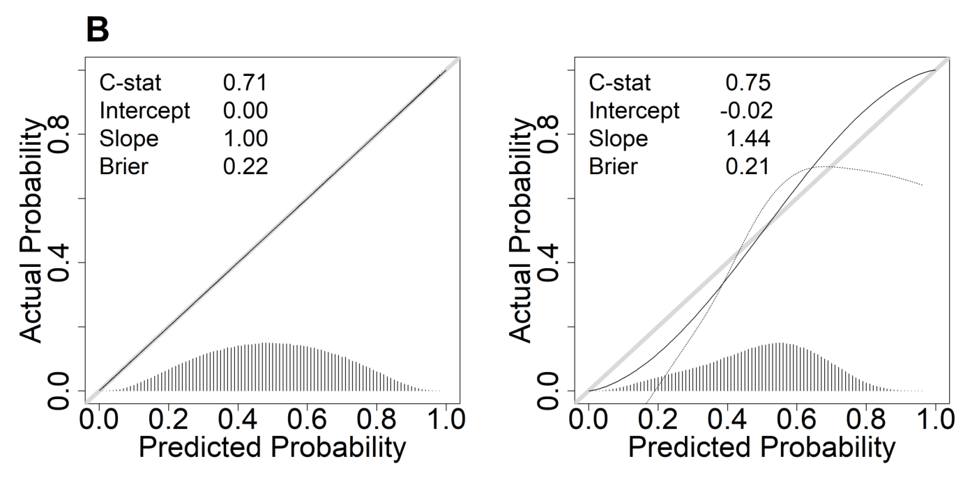
In situations of within-sample measurement error, i.e. in the re-estimated model, all calibration plots showed a calibration slope equal to , indicating perfect apparent calibration (Figure 1A-C). The apparent c-statistic and Brier score improved with decreasing random measurement error. In case of measurement heterogeneity across samples, i.e. in the transported model, similar changes in the c-statistic and Brier score were found. However, heterogeneous measurements led to a calibration slope , indicating that predictions were no longer valid (Figure 1D and 1F). When measurements at validation were less precise than at derivation, the calibration slope was , similar to statistical overfitting. When measurements at validation were more precise than at derivation, the calibration slope was , similar to statistical underfitting. More elaborate illustrations of the impact of measurement heterogeneity in large sample simulations, including effects of systematic and differential measurement heterogeneity, can be found in Appendix 1.
Although the total Brier score did not differ substantially between the re-estimated and transported model, examination of the large sample properties of the decomposed Brier score (Equation 7) indicated differences in the components between the procedures (Figure 2). In the re-estimated model, the calibration term equaled zero, and the total Brier score equaled the refinement term (Figure 2A). The Brier score increased with increasing random measurement error, indicating that accuracy decreased. In the transported model, changes in the refinement term were counterbalanced by changes in the calibration term. For example, when measurements at validation were less precise than at derivation, the spread in predicted probabilities increased (refinement term in Figure 2b decreased). A decrease in the refinement term under perfect calibration would indicate that overall accuracy of the model is improving, as predicted probabilities are closer to or . However, in the transported model this improvement was counterbalanced by a calibration term larger than zero, which indicates that predicted probabilities were too extreme compared to observed probabilities (Figure 2B).
Figure 1 and 2 illustrate that miscalibration is not introduced by measurement error per se, but rather by measurement heterogeneity across settings of derivation and validation. The discrepancy in calibration between model re-estimation and model transportation can be reduced to differences in the linear predictors of the recalibration models. In case of model re-estimation, the linear predictor is expressed by
| (9) |
indicating that the parameters and are estimated using the predictor values measured by strategy in the validation data. In the more realistic validation procedure in which the model is transported over different predictor measurement procedures, the linear predictor is expressed by
| (10) |
meaning that regression coefficients are estimated based on and that the model is validated using . This distinction in recalibration models sheds a different light on previous research into effects of measurement error on predictive performance. Khudyakov and colleagues derived analytically that calibration in a derivation sample is not affected by measurement error [15]. Since their findings are based on the assumption that the linear predictor is defined as in Equation (9), previous results on the impact of measurement error on predictive performance can be interpreted as effects on in-sample predictive performance [15, 23].
5 Predictive performance under measurement heterogeneity across settings
General patterns of predictive performance under measurement heterogeneity were examined in a set of Monte Carlo simulations in finite samples to evaluate their behavior under sampling variability. Simulations were performed in R version 3.3.1. [20] and our code is accessible online (see https://github.com/KLuijken/Prediction_Measurement_Heterogeneity_Predictor). We studied the predictive performance of a single- and a two-predictor binary logistic regression model. For the latter, we evaluated situations in which both predictors were measured heterogeneously across settings as well as situations in which one of the predictors was measured similar over settings. The data for the single-predictor model were generated from
The data for the two-predictor models were generated from
The correlation between predictors, , varied with , and . Both the -parameters in the two-predictor models have value in case or , and have value in case . We varied the values of the regression coefficients in order to keep the c-statistic of the data-generating models at an approximate value of and hence to compare predictive performance over models [16]. We recreated different measurement procedures of the predictors using different specifications of the general measurement error model (Equation 1). In the derivation sample, measurements corresponded to the random measurement error model (Equation 2), while in validation various measurement structures were recreated (see Table 2 for values of input parameters). All measurements contained at least some erroneous measurement variance to generate realistic scenarios.
In total, 432 scenarios were evaluated. For each scenario, a derivation sample () and a validation sample () were generated. We did not consider smaller sample sizes, since predictive performance measures are sensitive to statistical overfitting, which would complicate the interpretation of effects of measurement heterogeneity [4, 5]. The validation procedure was repeated 10,000 times for each simulation scenario. The number of events was around in each dataset, which exceeds the minimal requirement for validation studies [24, 25].
Simulation outcome measures
The simulation outcome measures were the average c-statistic, calibration slope, calibration-in-the-large coefficient, and Brier score. The c-statistic was computed using the somers2 function of the rms package [22]. The calibration slope was computed by regressing the observed outcome in the validation dataset on the linear predictor, as defined in Equation (9). We evaluated calibration graphically by plotting loess calibriation curves and overlaying the plots of all 10,000 resamplings [25, 26]. The calibration-in-the-large was computed as the intercept of the recalibration model, while using an offset for the linear predictor [1]. The empirical Brier score was computed using Equation (6). Additionally, we evaluated in-sample predictive performance as a reference for effects on out-of-sample performance.
5.1 Simulation results
Identical measurement error structures at derivation and validation resulted in consistent predictive performance across settings. All out-of-sample measures of predictive performance were affected by measurement heterogeneity. Effects on predictive performance measures were largest in the single-predictor model (Table 3). The two-predictor model in which one of the predictors was measured consistently over settings (Figure 3) outperformed the model in which none of the predictors were measured consistently across settings (Figure 4). Inspection of calibration plots confirmed all patterns of miscalibration discussed below (Supplementary Figure 1). By and large, the impact of correlation between predictors on other parameters was minimal since the correlation structure was equal across compared settings, hence, we show combined results in the figures.
5.1.1 Random measurement heterogeneity
When measurements were less precise at validation compared to derivation, i.e. when , the c-statistic decreased and Brier score increased at validation. In the single-predictor model, the c-statistic decreased from at derivation to at validation and the Brier score increased from at derivation to at validation (Table 3, bottom rows). Furthermore, the median calibration slope at validation was smaller than 1, ranging from in the single-predictor model. When measurements were more precise at validation compared to derivation, i.e. when , the c-statistic was increased, from to in the single-predictor model, and the Brier score was decreased, changing from to in the single-predictor model. However, the improved c-statistic and Brier score were accompanied by median calibration slopes greater than 1, ranging from in the single-predictor model (Table 3, top rows). Calibration-in-the-large was not affected by random measurement heterogeneity. Similar effects on predictive performance were observed for the two-predictor models, which are presented graphically in Figures 3 and 4.
5.1.2 Systematic measurement heterogeneity
When measurements at external validation changed by a constant compared to derivation, i.e. when and , the risk on observing the outcome was systematically overestimated, which is reflected in the negative value for calibration-in-the-large coefficient (Table 3). Changes in had little effect on the calibration slope and Brier score, and no apparent effect on the c-statistic. Multiplicative systematic measurement heterogeneity, i.e. , reinforced or counterbalanced effects of random measurement heterogeneity in the direction of the systematic measurement heterogeneity. When the association between and was relatively weak at validation, e.g. when , predictive performance deteriorated (black bars in Figures 3 and 4), whereas predictive performance improved when the association between and was relatively strong, e.g. when (gray bars in Figures 3 and 4).
5.1.3 Differential measurement heterogeneity
We highlight four specific scenarios in which the single-predictor model was derived under differential random measurement error, i.e. , and validated using non-differential measurements, and vice versa (Table 4). Differential measurement led to miscalibration at external validation in all scenarios. The c-statistic and Brier score at validation slightly improved when cases were measured less precise at derivation or more precise at validation. For example, when cases were measured less precise at derivation, i.e. , the c-statistic increased from to at validation and the Brier score decreased from to . However, the median calibration slope at validation was .
6 Discussion
Heterogeneity of predictor measurements across settings can have a substantial impact on the out-of-sample performance of a prediction model. When predictor measurements are more precise at derivation compared to validation, model discrimination and accuracy at validation deteriorate, and the provided predicted probabilities are too extreme, similar to when a model is overfitted with respect to the derivation data. When predictor measurements are less precise at derivation compared to validation, discrimination and accuracy at validation tend to improve, but the provided predicted probabilities are too close to the outcome prevalence, similar to statistical underfitting. These key findings of our study are summarized in Table 5. The current study emphasizes that a prediction model not only concerns the algorithm relating predictors to the outcome, but also depends on the procedures by which model input is measured, i.e. qualitative differences in data collection.
Measurement error is commonly thought not to affect the validity of prediction models, based on the general idea that unbiased associations between predictor and outcome are no prerequisite in prediction studies [12]. By taking the measurement error perspective, our study revealed that prediction research requires consideration of variation in measurement procedures across different settings of derivation and validation, rather than analyzing the amount of measurement error within a study. A recent systematic review by Whittle and colleagues demonstrated that measurement error was not acknowledged in many prediction studies, and pointed out the need to investigate consequences of measurement error in prediction research [27]. An important starting point for this research following from our study is that the generalizability of prediction models depends on the transportability of measurement structures.
Specification of measurement heterogeneity can help to explain discrepancies in predictive performance between derivation and validation setting in a pragmatic way. The relatedness between derivation and validation samples is generally quantified in terms of similarity in person-characteristics (also referred to as "case-mix"), and regression coefficients [1]. Previously proposed measures to express sample relatedness are the mean and spread of the linear predictor [7] or the correlation structure of predictors in both samples [28]. The information on sample relatedness can be incorporated in benchmark values of predictive performance to assess model transportability [6]. While regression coefficients and case-mix distributions clearly quantify sample relatedness, it is impossible to disentangle the sources of discrepancies from these statistical measures. For example, a decrease of the regression coefficients or the spread of the linear predictor at external validation could be due to differences across settings in either person-characteristics or the means by which these characteristics were measured. Moreover, less precise predictor measurements affect both the regression coefficients and the spread of the linear predictor, meaning that measurement heterogeneity can mask similarities and differences between the individuals in a derivation and validation sample. Knowledge of substantive differences between derivation and validation setting can help researchers determining to which extent the prediction model is transportable.
In theory, measurement error correction procedures could be applied to adjust for measurement heterogeneity when data on both and are available [10]. Alternatively, the degree of measurement heterogeneity could be quantified using the residual intraclass correlation (RICC), which expresses the clustering of measurements across physicians or centers [9]. Yet, we expect that the applicability of these methods in correcting for measurement heterogeneity will be limited not only due to the fact that individual patient data of both the derivation and validation set are required, but furthermore because it is infeasible to disentangle measurement parameters from other characteristics of the data. The main contribution of the taxonomy of measurement error models rises from its aptitude to conceptualize measurement heterogeneity across settings in pragmatic terms.
The following implications for prediction studies follow from our work. Ideally, prediction models are derived from predictor measurements that resemble measurement procedures in the intended setting of application. Data collection protocols that reduce measurement error to a minimum do not necessarily benefit the performance of the model as the precision of measurements will most likely not be obtained in validation (or application) settings. Deriving a prediction model from these precise measurements could result in miscalibration similar to model overfitting and reduced discrimination and accuracy at external validation. Furthermore, researchers should bear in mind the implications of using a ’readily available dataset’ for model derivation or validation as data quality directly affects predictive performance of the model. For instance, validating a model in a clinical trial dataset, in which measurements typically contain minimal measurement error, may increase measures of discrimination and accuracy, yet the model may provide predicted probabilities too close to the event rate due to miscalibration. Another example is the promising use of large routine care datasets for model validation [5, 29, 30]. Predictor measurement procedures may vary greatly within such datasets or differ from the procedures used to collect the data for the derivation study, which could increase the predictor measurement variance to a level that no longer resembles the amount of measurement variance within a clinical setting. Hence, rather than analyzing data because they are available, prediction models should be derived from and validated on datasets collected with measurement procedures that are in widespread use in the intended clinical setting. Finally, it is important to clearly report which measurement procedures were used for derivation or validation of a prediction model. The influential TRIPOD Statement has drawn attention to the importance of reporting measurement procedures [8]. Our findings indicate that descriptions of measurement procedures at model derivation are essential for proper external validation of the model. Likewise, validation studies ideally contain descriptions of deviations from measurements used at derivation, as these may introduce discrepancies in predictive performance.
Our study redefines the importance of predictor measurements in the context of prediction research. We highlight heterogeneity in predictor measurement procedures across settings as an important driver of unanticipated predictive performance at external validation. Preventing measurement heterogeneity at the design phase of a prediction study, both in development and validation studies, facilitates interpretation of predictive performance and benefits the transportability of the prediction model.
acknowledgements
The authors thank B. Rosche for his technical assistance.
disclaimer
All statements in this report, including its findings and conclusions, are solely those of the authors and do not necessarily represent the views of the Patient-Centered Outcomes Research Institute (PCORI), its Board of Governors or Methodology Committee.
conflict of interest
The authors declare that they have no conflict of interest.
data availability statement
Data sharing is not applicable to this article as no new data were created or analyzed in this study.
References
- [1] Steyerberg EW. Clinical prediction models: a practical approach to development, validation, and updating. Springer Science & Business Media; 2008.
- [2] Altman DG, Royston P. What do we mean by validating a prognostic model? Statistics in medicine 2000;19(4):453–473.
- [3] Collins GS, Ogundimu EO, Altman DG. Sample size considerations for the external validation of a multivariable prognostic model: a resampling study. Statistics in medicine 2016;35(2):214–226.
- [4] Steyerberg EW, Borsboom GJ, van Houwelingen HC, Eijkemans MJ, Habbema JDF. Validation and updating of predictive logistic regression models: a study on sample size and shrinkage. Statistics in medicine 2004;23(16):2567–2586.
- [5] Steyerberg EW, Uno H, Ioannidis JP, Van Calster B, et al. Poor performance of clinical prediction models: the harm of commonly applied methods. Journal of clinical epidemiology 2017;.
- [6] Vergouwe Y, Moons KG, Steyerberg EW. External validity of risk models: use of benchmark values to disentangle a case-mix effect from incorrect coefficients. American journal of epidemiology 2010;172(8):971–980.
- [7] Debray T, Moons KG, Ahmed I, Koffijberg H, Riley RD. A framework for developing, implementing, and evaluating clinical prediction models in an individual participant data meta-analysis. Statistics in Medicine 2013;32(18):3158–3180.
- [8] Collins GS, Reitsma JB, Altman DG, Moons KG. Transparent reporting of a multivariable prediction model for individual prognosis or diagnosis (TRIPOD): the TRIPOD statement. BMC medicine 2015;13(1):1.
- [9] Wynants L, Timmerman D, Bourne T, Van Huffel S, Van Calster B. Screening for data clustering in multicenter studies: the residual intraclass correlation. BMC medical research methodology 2013;13(1):128.
- [10] Keogh RH, White IR. A toolkit for measurement error correction, with a focus on nutritional epidemiology. Statistics in medicine 2014;33(12):2137–2155.
- [11] Steyerberg EW, Vickers AJ, Cook NR, Gerds T, Gonen M, Obuchowski N, et al. Assessing the performance of prediction models: a framework for some traditional and novel measures. Epidemiology (Cambridge, Mass) 2010;21(1):128.
- [12] Carroll RJ, Ruppert D, Stefanski LA, Crainiceanu CM. Measurement error in nonlinear models: a modern perspective. CRC press; 2006.
- [13] White E. Measurement error in biomarkers: sources, assessment, and impact on studies. IARC scientific publications 2011;(163):143–161.
- [14] Sackett DL. Bias in analytic research. In: The Case-Control Study Consensus and Controversy Elsevier; 1979.p. 51–63.
- [15] Khudyakov P, Gorfine M, Zucker D, Spiegelman D. The impact of covariate measurement error on risk prediction. Statistics in medicine 2015;34(15):2353–2367.
- [16] Austin PC, Steyerberg EW. Interpreting the concordance statistic of a logistic regression model: relation to the variance and odds ratio of a continuous explanatory variable. BMC medical research methodology 2012;12(1):82.
- [17] Brier GW. Verification of forecasts expressed in terms of probability. Monthey Weather Review 1950;78(1):1–3.
- [18] Spiegelhalter DJ. Probabilistic prediction in patient management and clinical trials. Statistics in medicine 1986;5(5):421–433.
- [19] Blattenberger G, Lad F. Separating the Brier score into calibration and refinement components: A graphical exposition. The American Statistician 1985;39(1):26–32.
- [20] Team R, R Development Core Team: R: a language and environment for statistical computing. Vienna: R Foundation for Statistical Computing; 2011; 2011.
- [21] Cox DR. Two further applications of a model for binary regression. Biometrika 1958;45(3/4):562–565.
- [22] Harrell Jr FE. rms: Regression Modeling Strategies. R package version 4.0-0. City 2013;.
- [23] Rosella LC, Corey P, Stukel TA, Mustard C, Hux J, Manuel DG. The influence of measurement error on calibration, discrimination, and overall estimation of a risk prediction model. Population health metrics 2012;10(1):20.
- [24] Vergouwe Y, Steyerberg EW, Eijkemans MJ, Habbema JDF. Substantial effective sample sizes were required for external validation studies of predictive logistic regression models. Journal of clinical epidemiology 2005;58(5):475–483.
- [25] Van Calster B, Nieboer D, Vergouwe Y, De Cock B, Pencina MJ, Steyerberg EW. A calibration hierarchy for risk models was defined: from utopia to empirical data. Journal of clinical epidemiology 2016;74:167–176.
- [26] Austin PC, Steyerberg EW. Graphical assessment of internal and external calibration of logistic regression models by using loess smoothers. Statistics in medicine 2014;33(3):517–535.
- [27] Whittle R, Peat G, Belcher J, Collins GS, Riley RD. Measurement error and timing of predictor values for multivariable risk prediction models are poorly reported. Journal of clinical epidemiology 2018;.
- [28] Kundu S, Mazumdar M, Ferket B. Impact of correlation of predictors on discrimination of risk models in development and external populations. BMC medical research methodology 2017;17(1):63.
- [29] Riley RD, Ensor J, Snell KI, Debray TP, Altman DG, Moons KG, et al. External validation of clinical prediction models using big datasets from e-health records or IPD meta-analysis: opportunities and challenges. bmj 2016;353:i3140.
- [30] Cook JA, Collins GS. The rise of big clinical databases. British Journal of Surgery 2015;102(2).
- [31] Mikula A, Hetzel S, Binkley N, Anderson P. Clinical height measurements are unreliable: a call for improvement. Osteoporosis International 2016;27(10):3041–3047.
- [32] Drawz PE, Ix JH. BP Measurement in Clinical Practice: Time to SPRINT to Guideline-Recommended Protocols. Journal of the American Society of Nephrology 2017;p. ASN–2017070753.
- [33] Genders TS, Steyerberg EW, Hunink MM, Nieman K, Galema TW, Mollet NR, et al. Prediction model to estimate presence of coronary artery disease: retrospective pooled analysis of existing cohorts. Bmj 2012;344:e3485.
- [34] Aubert CE, Folly A, Mancinetti M, Hayoz D, Donzé J. Prospective validation and adaptation of the HOSPITAL score to predict high risk of unplanned readmission of medical patients. Swiss medical weekly 2016;146:w14335.
- [35] Herder GJ, van Tinteren H, Golding RP, Kostense PJ, Comans EF, Smit EF, et al. Clinical prediction model to characterise pulmonary nodules: validation and added value of 18FDG PET. The use of 18FDG PET in NSCLC 2006;128:39.
- [36] Al-Ameri A, Malhotra P, Thygesen H, Plant PK, Vaidyanathan S, Karthik S, et al. Risk of malignancy in pulmonary nodules: a validation study of four prediction models. Lung Cancer 2015;89(1):27–30.
|
\headrow
Type of
predictor |
Examples of predictors | Examples of measurement heterogeneity |
| Anthropometric measurements |
Height
Weight Body circumference |
Guidelines on imaging decisions in osteoporosis care are established using standardized measurements of height, while in clinical practice height is measured using non-standardized techniques or self-reported values [31]. |
|
Physiological
measurements |
Blood pressure
Serum cholesterol HbA1c Fasting glucose |
In scientific studies, blood pressure is often measured by the average of multiple measurements performed under standardized conditions, while blood pressure measurements in practice deviate from protocol guidelines in various ways due to variability in available time and devices [32]. |
| Diagnosis |
Previous/current
disease |
The diagnosis ’hypertension’ can be defined as a blood pressure of mm Hg (without use of anti-hypertensive therapy) or as the use of anti-hypertensive drugs [33]. |
|
Treatment/
Exposure status |
Type of drug used
Smoking status Dietary intake |
The cut-off value for an ’increased length of stay in the hospital’ to predict unplanned readmission may depend on the country in which the model is evaluated [34]. |
| Imaging | Presence or size of tissue on ultrasound, MRI, CT or FDG PET scans | In scientific studies, review of FDG PET scans may be protocolized or performed by a single experienced nuclear medicine physician, blinded to patient outcome [35]. In routine practice, FDG PET scans may be reviewed under various systematics or by a multi-disciplinary team [36]. |
| \headrow | Factor values | |
|---|---|---|
| Derivation | 0 | |
| 1.0 | ||
| 0.5, 1.0, 2.0 | ||
| Validation | 0, 0.25 | |
| 0.5, 1.0, 2.0 | ||
| 0.5, 1.0, 2.0 | ||
| \headrow | \theadMeasurement structure | C-statistic | \theadCalibration | \theadCalibration-in- | Brier score | ||
|---|---|---|---|---|---|---|---|
| \headrow | \theadat validation | \theadDerivation | \theadValidation | \theadslope | \theadthe-large () | \theadDerivation | \theadValidation |
| , | 0.745 (0.033) | 0.590 (0.034) | 0.247 (0.153) | -0.002 (0.006) | 0.204 (0.012) | 0.281 (0.033) | |
| , | 0.745 (0.033) | 0.655 (0.045) | 0.380 (0.180) | 0.008 (0.014) | 0.204 (0.012) | 0.257 (0.031) | |
| , | 0.745 (0.033) | 0.726 (0.033) | 0.428 (0.125) | -0.009 (0.003) | 0.204 (0.012) | 0.232 (0.023) | |
| , | 0.745 (0.033) | 0.589 (0.034) | 0.247 (0.153) | -2.202 (0.643) | 0.204 (0.012) | 0.283 (0.032) | |
| , | 0.745 (0.033) | 0.655 (0.045) | 0.380 (0.180) | -2.210 (0.652) | 0.204 (0.012) | 0.258 (0.031) | |
| , | 0.745 (0.033) | 0.726 (0.033) | 0.428 (0.125) | -2.205 (0.651) | 0.204 (0.012) | 0.233 (0.023) | |
| , | 0.700 (0.068) | 0.635 (0.069) | 0.812 (0.291) | 0.001 (0.006) | 0.217 (0.020) | 0.235 (0.015) | |
| , | 0.700 (0.068) | 0.700 (0.068) | 1.000 (0.000) | 0.001 (0.008) | 0.217 (0.020) | 0.218 (0.020) | |
| , | 0.700 (0.068) | 0.753 (0.042) | 0.955 (0.377) | -0.002 (0.013) | 0.217 (0.020) | 0.204 (0.014) | |
| , | 0.700 (0.068) | 0.635 (0.069) | 0.811 (0.293) | -1.529 (1.027) | 0.217 (0.020) | 0.237 (0.014) | |
| , | 0.700 (0.068) | 0.700 (0.068) | 1.002 (0.002) | -1.530 (1.033) | 0.217 (0.020) | 0.219 (0.019) | |
| , | 0.700 (0.068) | 0.753 (0.042) | 0.955 (0.377) | -1.526 (1.024) | 0.217 (0.020) | 0.205 (0.013) | |
| , | 0.655 (0.045) | 0.681 (0.045) | 3.147 (1.991) | 0.003 (0.007) | 0.230 (0.011) | 0.234 (0.009) | |
| , | 0.655 (0.045) | 0.745 (0.034) | 3.106 (1.563) | 0.000 (0.006) | 0.230 (0.011) | 0.220 (0.014) | |
| , | 0.655 (0.045) | 0.781 (0.014) | 2.160 (0.969) | 0.005 (0.009) | 0.230 (0.011) | 0.203 (0.013) | |
| , | 0.655 (0.045) | 0.681 (0.045) | 3.156 (2.001) | -0.846 (0.528) | 0.230 (0.011) | 0.235 (0.008) | |
| , | 0.655 (0.045) | 0.745 (0.034) | 3.102 (1.559) | -0.846 (0.532) | 0.230 (0.011) | 0.221 (0.013) | |
| , | 0.655 (0.045) | 0.781 (0.014) | 2.159 (0.967) | -0.851 (0.535) | 0.230 (0.011) | 0.203 (0.013) | |
| \headrow | C-statistic | Calibration | Brier score | |||
|---|---|---|---|---|---|---|
| \headrow Differential measurement error at… | Derivation | Validation | slope | Derivation | Validation | |
| Derivation | 0.730 (0.011) | 0.707 (0.012) | 0.780 (0.071) | 0.209 (0.004) | 0.219 (0.004) | |
| 0.655 (0.012) | 0.707 (0.012) | 1.856 (0.208) | 0.231 (0.003) | 0.223 (0.002) | ||
| Validation | 0.706 (0.012) | 0.730 (0.011) | 1.293 (0.120) | 0.217 (0.003) | 0.211 (0.003) | |
| 0.706 (0.012) | 0.655 (0.012) | 0.547 (0.061) | 0.217 (0.004) | 0.237 (0.005) | ||
| \headrow | Predictive performance at validation | ||||
| \headrowPredictor measurements at validation | Discrimination | Calibration-in-the-large | Calibration slope | Overall accuracy | |
| Less precise compared to derivation; | Deteriorated | - | Deteriorated | ||
| More precise compared to derivation; | Improved | - | Improved | ||
| Weaker association with actual predictor value, while | |||||
| - less precise compared to derivation; | , | Stronger deterioration | - | Stronger | Stronger deterioration |
| - more precise compared to derivation; | , | Less improvement | - | Stronger | Less improvement |
| Stronger association with actual predictor value, while | |||||
| - less precise compared to derivation; | , | Less deterioration | - | Less | Less deterioration |
| - more precise compared to derivation; | , | Stronger improvement | - | Less | Stronger improvement |
| Increased by a constant relative to derivation. | - | - | - | ||


MV = measurement variance of the predictor measurement used for model validation relative to the predictor measurement used for derivation. The data generating mechanism corresponded perfectly to the estimated logistic regression model. The top rows show calibration plots of a single-predictor model that is fitted using predictor measurement and validated by re-estimating the model on the same data using . The bottom rows show situations where the same model is transported from derivation to validation setting, specifically, the model (D) is derived using and validated using , (E) is derived and validated using , and (F) is derived using and validated using . The calibration plots show the calibration slope (black line) and predicted probability frequencies (bottom-histograms) for situations in which the predictor measurement variance at validation equals 200% (A,D), 100% (B,E), or 50% (C,F) of the predictor measurement variance at derivation. The val.prob function from the rms package was used to compute the simulation outcome measures and to generate the calibration plots [22], where we edited the legend format settings in the plot to improve readability.
MV = measurement variance of the predictor measurement used for model validation relative to the predictor measurement used for derivation. The data generating mechanism corresponded perfectly to the estimated logistic regression model. The plot displays the large sample properties of the components of the Brier score (Equation 7) under increasing random predictor measurement variance at validation, corresponding to the random measurement error model (Equation 2). The left panel shows the Brier score for a single-predictor logistic regression model that is fitted using predictor measurement and validated by re-estimating the model on the same data using . The right panel shows transportation from at derivation to at validation (upto %MV = 100) and transportation from at derivation to at validation (from %MV = 100 onwards).
Mean c-statistic, median calibration slope and mean Brier score averaged over repetitions with interquartile range and 95% confidence interval for a two-predictor model where one of the predictors is measured consistent across settings, while the other is measured heterogeneously. Horizontal bars indicate performance measures at model derivation, while boxes indicate performance at external validation. The predictor measurement structure in the derivation set (n= ) corresponds to the random measurement error model (Equation 2). In the validation set (n= ), predictor measurements consist of varying structures under Equation (1).
Mean c-statistic, median calibration slope and mean Brier score averaged over repetitions with interquartile range and 95% confidence interval of a two-predictor logistic regression model in which both predictors are measured heterogeneously across settings. Horizontal bars indicate performance measures at model derivation, while boxes indicate performance at external validation. Measurements in the derivation set (n= ) are recreated using Equation (2), which corresponds to the random measurement error model. In the validation set (n= ), measurements correspond to various measurement structures under Equation (1).
Appendix 1
In this appendix, the general effects of measurement heterogeneity on external predictive performance are illustrated in large sample simulations ().
Simulation design
We examined the predictive performance of a single-predictor binary logistic regression model. The data were generated from
and where reflects the true (often unobserved) underlying value of the predictor. The dataset contained two measurements of the predictor , which were recreated under the general measurement error model (Equation 1). The first measurement, denoted , was used to derive the logistic regression model and corresponded to the random error model (Equation 2). The other measurement, , was used to validate the model and corresponded to various measurement structures under the general measurement error model. This validation procedure implies that the model is validated in its original sample, hence, in absence of all other impacts on model transportability. The val.prob function from the rms package in R was used to compute the simulation outcome measures and to generate the calibration plots [22], where we edited the legend format settings in the plot to improve readability.
Simulation results
In line with expectations, the predictive performance at validation corresponded perfectly to the predictive performance at derivation when the predictor was measured consistently over settings. The impact on predictive performance when measurements were heterogeneous is described below.
Random measurement heterogeneity
When the measurement at validation, in , was less precise than at derivation, in , i.e. when , the c-statistic decreased from at derivation to at validation and the Brier score increased from to , indicating a loss in discriminatory power and accuracy. Furthermore, the calibration slope was , similar to statistical overfitting (Figure 5b). When the measurement was more precise than , i.e. when , the c-statistic increased from to , and the Brier score decreased from to . However, the improved c-statistic and Brier score were accompanied by a calibration slope of , similar to statistical underfitting (Figure 5d). Calibration-in-the-large was not affected by random measurement heterogeneity.
Systematic measurement heterogeneity
Additive systematic measurement heterogeneity, i.e. , resulted in systematic overestimation of the outcome, which is reflected in the negative value for calibration-in-the-large coefficient, (Figure 6c). Changes in had no apparent effect on the calibration slope, c-statistic, and Brier score. Multiplicative systematic measurement heterogeneity at validation, in , i.e. , in combination with random measurement error led to a calibration slope . The impact on the c-statistic and the Brier score was in the direction of association between and . When this association was relatively weak, e.g. when , the c-statistic decreased from to and the Brier score increased from to (Figure 7b). When the association between and was relatively strong, e.g. when , the c-statistic improved from to and the Brier score improved from to (Figure 7d).
Differential measurement heterogeneity
All forms of differential measurement of cases and non-cases led to miscalibration at external validation. For example, when measurement of cases was less precise at validation, in , i.e. , the calibration slope at validation was . The c-statistic decreased from to , the Brier score increased from to (Figure 8a). In case of systematic differential measurement of cases and non-cases, when the association between and in cases was weaker in , i.e. , the c-statistic decreased from to , the Brier score increased from to , and the calibration slope was (Figure 8c).
Inverse effects on predictive performance were found when cases and non-cases were measured differentially at derivation, in . When measurement of cases was less precise at derivation, i.e. , the c-statistic increased from to , the Brier score decreased from to , and the calibration slope at validation was (Figure 9b). When the association between and in cases was weaker at derivation, in , i.e. , the c-statistic improved from to , the Brier score improved from to , and the calibration slope was (Figure 9c).
Random measurement heterogeneity

| A. , | where and . | |
| B. , | where and . | Measurements are less precise at validation, i.e. . |
| C. , | where and . | Measurements consistent across settings, i.e. . |
| D. , | where . | Measurements are more precise at validation, i.e. . |
Additive systematic measurement heterogeneity

| A. , | where and . | |
| B. , | where , and . | Measurements are equal across settings. |
| C. , | where , and . | Measurements are shifted from by a constant. |
Multiplicative systematic measurement heterogeneity

| A. , | where , and . | |
| B. , | where , and . | The association - is weaker at validation. |
| C. , | where , and . | The association - is equal across settings. |
| D. , | where , and . | The association - is stronger at validation. |
Differential measurement heterogeneity at validation


| A. , | where and . | Measurements of cases are less precise at validation. |
| B. , | where and . | Measurements of cases are more precise at validation. |
| C. , | where , and . | Associations between and in cases are weaker at validation. |
Differential measurement heterogeneity at derivation


| A. , | where and . | Measurements of cases are more precise at derivation. |
| B. , | where and . | Measurements of cases are less precise at derivation. |
| C. , | where , and . | Associations between and in cases are weaker at derivation. |
Supplementary Figure 1
