Matrix Completion from Non-Uniformly Sampled Entries
Abstract
In this paper, we consider matrix completion from non-uniformly sampled entries including fully observed and partially observed columns. Specifically, we assume that a small number of columns are randomly selected and fully observed, and each remaining column is partially observed with uniform sampling. To recover the unknown matrix, we first recover its column space from the fully observed columns. Then, for each partially observed column, we recover it by finding a vector which lies in the recovered column space and consists of the observed entries. When the unknown matrix is low-rank, we show that our algorithm can exactly recover it from merely entries, where is the rank of the matrix. Furthermore, for a noisy low-rank matrix, our algorithm computes a low-rank approximation of the unknown matrix and enjoys an additive error bound measured by Frobenius norm. Experimental results on synthetic datasets verify our theoretical claims and demonstrate the effectiveness of our proposed algorithm.
1 Introduction
Recently, low-rank matrix completion has received a great deal of interests due to its theoretical advances (Candes and Recht, 2009; Keshavan et al., 2010), as well as its application to a wide range of real-world problems, including recommendation (Goldberg et al., 1992; Yi et al., 2017; Yi et al., 2013a), sensor networks (Biswas et al., 2006), computer vision (Cabral et al., 2011), security (Yi et al., 2014), human resource (Horesh et al., 2016), crowdsourcing (Yi et al., 2012c; Yi et al., 2012a), and machine learning (Jalali et al., 2011; Yi et al., 2012b; Yi et al., 2013b). Let be an unknown matrix of size , and we assume without loss of generality. The information available about is a sampled set of entries , where and . Our goal is to recover as precisely as possible.
Most of the previous work in matrix completion assumes the entries in are Sampled Uniformly at Random (abbr. SUR) (Candes and Tao, 2010; Recht, 2011). However, this assumption may be violated in real-world applications. For example, in image annotations, where the data is a matrix between images and tags, it is common to observe entire columns that correspond to well-studied categories and entire rows that correspond to labeled images. In medical diagnosis, where the data is a matrix between patients and medical measurements, it is possible to collect entire columns that correspond to inexpensive measurements and entire rows that correspond to important patients. Thus, it is natural to ask whether it is possible to recover an unknown matrix from some rows and/or columns.
Perhaps a bit surprising, answers to the above problem can be found in the recent developments of CUR matrix decomposition. The goal of CUR decomposition is to approximate a matrix by , where is estimated according to specific methods, and contain some rows and columns of , respectively. While most algorithms for CUR require that is known beforehand, there are several exceptions, including a Nyström-type algorithm (abbr. Nyström) (Drineas et al., 2008) and CUR (Xu et al., 2015). CUR aims to recover an unknown matrix from
| (1a) | ||||
| (1b) | ||||
| (1c) | ||||
Nyström can approximate the unknown matrix by only using (1a) and (1b).
Along this line of research, we study the problem of matrix completion from non-uniformly sampled entries, and show that the condition in (1c) can be dropped and the condition in (1b) can be relaxed. Specifically, we assume that the learner observes
| (2a) | ||||
| (2b) | ||||
Note that in (2b), we only require entries from the same column are SUR, and entries from different columns could be sampled jointly. In particular, the condition in (1b) is a special case of (2b). Thus, our observation model is more general than both Nyström (Drineas et al., 2008) and CUR (Xu et al., 2015). An illustration of our observation model is given in Figure 1. While our algorithm can handle both cases in Figure 1(a) and Figure 1(b), Nyström is limited to Figure 1(a), and CUR requires even more information than Nyström.

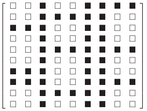
Our recovery algorithm consists of two simple steps:
- 1.
recover the column space of from the observed columns, and
- 2.
recover each partially observed column by finding a vector that lies in the recovered column space and consists with the observed entries.
Let be the rank of the unknown matrix . When is of low-rank and satisfies the incoherence condition, it can be recovered perfectly when we observe columns completely and entries for each remaining column. Thus, the sample complexity is , which is slightly better than the of the conventional matrix completion (Recht, 2011). Furthermore, when the unknown matrix is the sum of a low-rank matrix and a Gaussian noise matrix , we establish an upper bound measured by Frobenius norm for recovering its best rank- approximation , under the assumption that the top eigenspaces of and the column norm of are incoherent.
2 Related Work
In this section, we briefly review the related work in matrix completion and low-rank matrix approximation.
Matrix Completion Matrix completion refers to the problem of recovering a low-rank matrix based on partially observed entries, and motivates a series of work (Candes and Recht, 2009; Candes and Tao, 2010; Keshavan et al., 2010; Gross, 2011; Recht, 2011) which can exactly recover a rank- matrix of size from uniformly observed entries based on the framework of convex optimization under the incoherence condition. Recently, two improvements (Krishnamurthy and Singh, 2013; Xu et al., 2015) have been proposed to further reduce the sample complexity by adopting better strategies to observe necessary entries rather than uniform sampling from the whole unknown matrix.
Specifically, the algorithm proposed by Krishnamurthy and Singh (2013) needs to observe a set of columns sampled with adaptive sensing strategy and a set of rows sampled uniformly at random, and its sample complexity is . We note that two recent work (Krishnamurthy and Singh, 2014; Balcan and Zhang, 2016) improves the sample complexity of this algorithm to and respectively. Although its sample complexity may be slightly better than our , this algorithm cannot handle the observation model in Figure 1(b). As mentioned before, CUR (Xu et al., 2015) requires more conditions as it needs to observe a set of entries, columns, and rows sampled uniformly at random. Compared with our algorithm, the observation model of CUR+ is too restrictive, although it has a slightly better sample complexity.
Low-Rank Matrix Approximation Low-rank matrix approximation refers to the problem of approximating a given matrix by another matrix of rank not greater than a specified rank where . It arises from numerous applications such as latent semantic indexing (Deerwester et al., 1990), DNA microarray analysis (Troyanskaya et al., 2001), face recognition (Turk and Pentland, 1991), and web search (Kleinberg, 1999). Although singular value decomposition (SVD) can be used to find an optimal solution for this problem in a well-defined sense, it is not scalable since its memory and time complexities are superlinear w.r.t. and . To address this issue, several efficient algorithms based on norm sampling (Frieze et al., 2004; Drineas et al., 2006) and adaptive sampling (Deshpande et al., 2006; Deshpande and Vempala, 2006) have been proposed. Although these algorithms can find a good low-rank approximation, they need to observe the entire matrix.
To deal with missing data, Achlioptas and Mcsherry (2007) propose entrywise subsampling whose main idea is to construct an unbiased estimator of the unknown matrix and compute the SVD of the estimator. This algorithm has shortcomings that it cannot exactly recover a low-rank matrix and cannot capture the real column space of the unknown matrix. Although Nyström (Drineas et al., 2008) can capture the actual column and row space of the unknown matrix, it is limited to solve the problem illustrated in Figure 1(a). CUR, which requires more restrictive observation model, focus on the setting that the unknown matrix has skewed singular value distribution when it is of full-rank. Even so, CUR requires nearly the entire matrix for finding a good low-rank approximation, as discussed by Xu et al. (2015). The adaptive strategy and its variant have also been applied to computing a better low-rank approximation for an unknown noisy low-rank matrix (Krishnamurthy and Singh, 2013; Wang and Singh, 2015). However, these algorithms rely on sampling strategies that require more than one pass over the unknown matrix and their bounds have a poor dependence on failure probability , i.e., , which significantly limits their applications when columns are uniformly sampled, or the unknown matrix can only be sampled with one pass.
3 Main Results
In this section, we present our algorithms and the corresponding theoretical results.
3.1 The Proposed Algorithm
For a matrix , let and denote the -th row and -th column of , respectively. For a set , the vector contains elements of vector indexed by . Similarly the matrix has rows of matrix indexed by .
Let be the matrix to be recovered. Let be a probability distribution used to randomly sample columns where . To approximate , we first sample columns from and construct , where we pick with and set for Let be the target rank and . We calculate the top- left singular vectors of denoted by that is approximately the column space of . For each of the rest columns , we sample a set of entries uniformly at random with replacement, denoted by . We then solve the following optimization problem
| (3) |
to recover this column by , where is the optimal solution. Because the problem (3) has a closed-form solution , we have
The detailed procedures are summarized in Algorithm 1.
3.2 Theoretical Guarantees
Given , let and where and are the top- left and right singular vectors of , respectively. Define projection operators , . The incoherence measure for and is defined as
Similarly, the incoherence measure for is defined as
In the following, we first consider the low-rank case where , and then prove a general result for any fixed probability distribution .
Theorem 1.
Let be the probability distribution used to randomly sample columns and , where . Assume , , and . With a probability at least , Algorithm 1 recovers exactly.
From Theorem 1, we find that the lower bound of depends on the probability distribution. To minimize the threshold , we set
| (4) |
which corresponds to uniform sampling. From this perspective, uniform sampling is a useful strategy for recovering the low-rank matrix though it is very simple. By combining (4) and Theorem 1, we provide the following corollary for our Algorithm 1.
Corollary 1.
Assume , and . With a probability at least , Algorithm 1 with uniform sampling recovers exactly.
Corollary 1 implies the sample complexity of Algorithm 1 with uniform sampling is . Although it is slightly worse than the previous best result (Xu et al., 2015; Balcan and Zhang, 2016), it is much more general. Besides, it is easy to verify that our sample complexity can be further reduced to too when we sample the same as Xu et al. (2015) or Balcan and Zhang (2016).
In practice, the low-rank matrix may be corrupted by noise, and the matrix could be of full-rank. To handle the general setting, we assume that where is a low-rank matrix and is a random matrix with entries independently drawn from . Let where are the top- left singular vectors of . Our goal is to calculate a low-rank approximation of . To this end, we introduce a new incoherence measure The following theorem establishes the error guarantee of Algorithm 1.
Theorem 2.
Assume that where and is a random matrix with entries independently drawn from . Suppose that and . Let be the output of our Algorithm 1 with uniform sampling. Then with probability at least , we have
provided that and .
Theorem 2 shows that with an observation, Algorithm 1 with uniform sampling can achieve additive approximation error with an overwhelming probability. For comparison, we note that Wang and Singh (2015) achieve a relative error guarantee as
with a probability and sample complexity . However, their bounds have a poor dependence on the failure probability , i.e., , and their algorithm requires more than one pass over the unknown matrix. Xu et al. (2015) show that CUR achieves a similar relative error guarantee measured by spectral norm with high probability. Nevertheless, even the unknown matrix has skewed singular value distribution, CUR requires nearly the entire matrix, i.e., observed entries.
4 Analysis
In this section, we prove Theorems 1 and 2 by introducing several key lemmas. We defer the detailed proofs to the supplementary material due to space limitation.
4.1 Proof of Theorem 1
For each column not included in , if and is invertible, we can write , where . Thus, we have
This means that each column can be recovered exactly under two conditions: and is invertible. Therefore, based on the following two lemmas, we show that our Algorithm 1 with the assumptions in Theorem 1 satisfies these two conditions.
Lemma 1.
Let be the probability distribution used to randomly sample column and , where . Assume has rank , with a probability at least , we have
provided that
Lemma 2.
With a probability at least , we have
provided that .
By combining Lemma 1 and the fact that has rank , when and with a probability at least , we have , which means . Note that is composed of selected and rescaled columns of . Hence , which directly implies that and , . Then, according to Lemma 2 and the union bound, we have with probability at least for all column with the fact . Note that this means all are invertible with probability at least . Using union bound again, we can exactly recover with a probability at least . Let , we get .
4.2 Proof of Theorem 2
Let , where and . Besides Theorem 2, we further introduce several lemmas that are central to our analysis.
Lemma 3.
(Lemma in Krishnamurthy and Singh (2013)) For a vector , let Let , where and . With probability at least , we have
where .
Lemma 4.
For a vector , let Assume that where and is a random matrix with entries independently drawn from . Suppose , . With probability at least , we have
| (5) |
and with probability at least , we have
| (6) |
for all partially observed .
Lemma 5.
Due to Lemma 2 and the union bound, with a probability at least , we have
provided that for all . So with a probability at least , for all columns, we have
provided that
Summing over all columns, we have
According to Lemma 5, if , then with probability at least ,
which leads to
Now we check whether the conditions of and are satisfied. First, the condition means . Then, the condition can further derive since
5 Experiments
In this section, we first verify the theoretical result in Corollary 1, i.e., Algorithm 1 with uniform sampling has a dependence of sample complexity on and . To this end, we evaluate the performance of Algorithm 1 with uniform sampling by comparing it against Nyström (Drineas et al., 2008) for computing a low-rank approximation to a noisy low-rank matrix.
5.1 Verifying the Dependences on and
We will verify the sample complexity in Corollary 1, i.e., and .
Settings
Here we adopt the similar settings as in Xu et al. (2015). We study square matrices of different sizes and ranks, with varied in , and varied in . For each special and , we search for the smallest and that can lead to almost exact recovery of the target matrix, i.e., in all independent trials. To create the rank- matrix , we randomly generate matrix and , where each entry of and is drawn independently at random from , and is given by . Under this construction scheme, the difference among the incoherence for different sized matrices is relatively small (from to ), so we ignore the impact of in our analysis.
Results
The dependence of minimal on and is shown in Figures 2(a) and (b), which plot against and , respectively. We can find that has a linear dependence on instead of . In addition, we also find that is almost independent from the matrix size . Figures 2(c) and (d) plot , the minimum number of observed entries for each column, against and . We can see that also has a linear dependence on instead of . According to Theorem 1, the requirement on depends on , but we find that is almost independent from the matrix size . This suggests that is the worst sample complexity, where is caused by the union bound, and could be independent from in practice.


5.2 Comparison with Baseline Method for Low Rank Approximation
Because Theorem 2 shows that Algorithm 1 with uniform sampling enjoys additive error bound measured by Frobenius norm. To verify Theorem 2, we compare Algorithm 1 with uniform sampling against Nyström (Drineas et al., 2008) with uniformly sampled rows and columns to show that our algorithm with more general observation model can also perform well. Since CUR requires the observed entries to meet more conditions, which limits its application, we do not include it in the comparison. We note that algorithms based on approximate adaptive sampling and approximate norm sampling (Krishnamurthy and Singh, 2013; Wang and Singh, 2015) may yield better approximation, but these algorithms do not sample columns uniformly and can not deal with the unknown matrix with only one pass. Therefore, they are also not included in the comparison.


Settings
Following the experiment strategy of Xu et al. (2015), we set the number of uniformly sampled columns and rows to and respectively for Nyström, where is the target rank and is a parameter. For the sake of fairness, when our algorithm observed columns and entries for each partially observed column, we set such that Nyström observes the same number of entries with our algorithm. According to Theorem 2, our algorithm should run with parameters and . Because and is expected to be small such that , we set for our algorithm in the following experiments. We study square matrices of size which are the sum of a low-rank matrix and a Gaussian noise matrix , where each entry of is drawn independently at random from . To create the rank- matrix , we randomly generate matrix and , where each entry of and is drawn independently at random from , and is given by . Under this construction scheme, the incoherence is small for different and (from minimum 2.2929 to maximum 2.6792).
Results
We repeat each experiment times and report the average and the standard deviation of the approximation error in Figure 3. We find that our algorithm outperforms Nyström for different and , when they observe the same number of entries. Compared with Nyström, besides more general observation requirements, an additional advantage of our algorithm is explicitly extracting and exploiting the low-rank space of the sampled columns, which makes our algorithm more accurate and robust.
6 Conclusion
In this paper, we propose an algorithm to address the matrix completion problem from non-uniformly sampled entries. According to our theoretical analysis, our algorithm can perfectly recover a low-rank matrix with observed entries, despite the probability distribution used to sample columns. Specifically, our algorithm with uniform sampling only needs number of observed entries to perfectly recover a low-rank matrix. Furthermore, for noisy low-rank matrix, we show that the low-rank approximation computed by our algorithm with uniform sampling enjoys additive error bound measured by Frobenius norm. Numerical experiments verify our theoretical claims and demonstrate the effectiveness of our proposed algorithm.
References
- Achlioptas and Mcsherry (2007) Dimitris Achlioptas and Frank Mcsherry. Fast computation of low-rank matrix approximations. Journal of the ACM, 54(2):1–19, 2007.
- Balcan and Zhang (2016) Maria-Florina F. Balcan and Hongyang Zhang. Noise-tolerant life-long matrix completion via adaptive sampling. In Advances in Neural Information Processing Systems 29, pages 2955–2963, 2016.
- Biswas et al. (2006) Pratik Biswas, Tzu-Chen Lian, Ta-Chung Wang, and Yinyu Ye. Semidefinite programming based algorithms for sensor network localization. ACM Transactions on Sensor Networks, 2(2):188–220, 2006.
- Cabral et al. (2011) Ricardo S. Cabral, Fernando Torre, Joao P. Costeira, and Alexandre Bernardino. Matrix completion for multi-label image classification. In Advances in Neural Information Processing Systems 24, pages 190–198, 2011.
- Candes and Recht (2009) Emmanuel J. Candes and Benjamin Recht. Exact matrix completion via convex optimization. Foundations of Computational Mathematics, 9(6):717–772, 2009.
- Candes and Tao (2010) Emmanuel J. Candes and Terence Tao. The power of convex relaxation: Near-optimal matrix completion. IEEE Transactions on Information Theory, 56(5):2053–2080, 2010.
- Deerwester et al. (1990) Scott Deerwester, Susan T. Dumais, George W. Furnas, Thomas K. Landauer, and Richard Harshman. Indexing by latent semantic analysis. Journal of the American Society for Information Science, 41(6):391–407, 1990.
- Deshpande and Vempala (2006) Amit Deshpande and Santosh Vempala. Adaptive sampling and fast low-rank matrix approximation. Approximation, Randomization, and Combinatorial Optimization. Algorithms and Techniques, pages 292–303, 2006.
- Deshpande et al. (2006) Amit Deshpande, Luis Rademacher, Santosh Vempala, and Grant Wang. Matrix approximation and projective clustering via volume sampling. In Proceedings of the 17th annual ACM-SIAM symposium on Discrete algorithm, pages 1117–1126, 2006.
- Drineas et al. (2006) P Drineas, R Kannan, and M W Mahoney. Fast monte carlo algorithms for matrices ii: Computing a low-rank approximation to a matrix. SIAM Journal on computing, 36(1):158–183, 2006.
- Drineas et al. (2008) Petros Drineas, Michael W. Mahoney, and S. Muthukrishnan. Relative-error CUR matrix decompositions. SIAM Journal on Matrix Analysis and Applications, 30(2):844–881, 2008.
- Frieze et al. (2004) Alan Frieze, Ravi Kannan, and Santosh Vempala. Fast monte-carlo algorithms for finding low-rank approximations. Journal of the ACM, 51(6):1025–1041, 2004.
- Goldberg et al. (1992) David Goldberg, David Nichols, Brian M. Oki, and Douglas Terry. Using collaborative filtering to weave an information tapestry. Communications of the ACM, 35(12):61–70, 1992.
- Gross (2011) David Gross. Recovering low-rank matrices from few coefficients in any basis. IEEE Transactions on Information Theory, 57(3):1548–1566, 2011.
- Horesh et al. (2016) Raya Horesh, Kush R Varshney, and Jinfeng Yi. Information retrieval, fusion, completion, and clustering for employee expertise estimation. In 2016 IEEE International Conference on Big Data, pages 1385–1393, 2016.
- Jalali et al. (2011) Ali Jalali, Yudong Chen, Sujay Sanghavi, and Huan Xu. Clustering partially observed graphs via convex optimization. In Proceedings of the 28th International Conference on Machine Learning, pages 1001–1008, 2011.
- Keshavan et al. (2010) Raghunandan H. Keshavan, Andrea Montanari, and Sewoong Oh. Matrix completion from a few entries. IEEE Transactions on Information Theory, 56(6):2980–2998, 2010.
- Kleinberg (1999) Jon M. Kleinberg. Authoritative sources in a hyperlinked environment. Journal of the ACM, 46(5):604–632, 1999.
- Krishnamurthy and Singh (2013) Akshay Krishnamurthy and Aarti Singh. Low-rank matrix and tensor completion via adaptive sampling. In Advances in Neural Information Processing Systems 26, pages 836–844, 2013.
- Krishnamurthy and Singh (2014) Akshay Krishnamurthy and Aarti Singh. On the power of adaptivity in matrix completion and approximation. arXiv:1407.3619, 2014.
- Laurent and Massart (2000) B. Laurent and P. Massart. Adaptive estimation of a quadratic functional by model selection. The Annals of Statistics, 28(5):1302–1338, 2000.
- Recht (2011) Benjamin Recht. A simpler approach to matrix completion. Journal of Machine Learning Research, 12:3413–3430, 2011.
- Smale and Zhou (2007) Steve Smale and Ding-Xuan Zhou. Learning theory estimates via integral operators and their approximations. Constructive Approximation, 26(2):153–172, 2007.
- Tropp (2012) J A Tropp. User-friendly tail bounds for sums of random matrices. Foundations of computational mathematics, 12(4):389–434, 2012.
- Troyanskaya et al. (2001) Olga Troyanskaya, Michael Cantor, Gavin Sherlock, Pat Brown, Trevor Hastie, Robert Tibshirani, David Botstein, and Russ B. Altman. Missing value estimation methods for dna microarrays. Bioinformatics, 17(6):520–525, 2001.
- Turk and Pentland (1991) Matthew Turk and Alex Pentland. Eigenfaces for recognition. Journal of cognitive neuroscience, 3(1):71–86, 1991.
- Vershynin (2010) R. Vershynin. Introduction to the non-asymptotic analysis of random matrices. arXiv:1011.3027, 2010.
- Wang and Singh (2015) Yining Wang and Aarti Singh. Column subset selection with missing data via active sampling. In Proceedings of the 18th International Conference on Artificial Intelligence and Statistics, 2015.
- Xu et al. (2015) Miao Xu, Rong Jin, and Zhi-Hua Zhou. CUR algorithm for partially observed matrices. In Proceedings of the 32nd International Conference on Machine Learning, pages 1412–1421, 2015.
- Yi et al. (2012a) J. Yi, R. Jin, A. K Jain, and S. Jain. Crowdclustering with sparse pairwise labels: A matrix completion approach. In Proceedings of the 4th AAAI Workshop on Human Computation, pages 47–53, 2012a.
- Yi et al. (2012b) J. Yi, T. Yang, R. Jin, A. K Jain, and M. Mahdavi. Robust ensemble clustering by matrix completion. In Proceedings of the 12th IEEE International Conference on Data Mining, pages 1176–1181, 2012b.
- Yi et al. (2013a) J. Yi, R. Jin, S. Jain, and A. Jain. Inferring users’ preferences from crowdsourced pairwise comparisons: A matrix completion approach. In Proceedings of the 1st AAAI Conference on Human Computation and Crowdsourcing, pages 207–215, 2013a.
- Yi et al. (2012c) Jinfeng Yi, Rong Jin, Anil K. Jain, Shaili Jain, and Tianbao Yang. Semi-crowdsourced clustering: Generalizing crowd labeling by robust distance metric learning. In Advances in Neural Information Processing Systems 25, pages 1781–1789, 2012c.
- Yi et al. (2013b) Jinfeng Yi, Lijun Zhang, Rong Jin, Qi Qian, and Anil Jain. Semi-supervised clustering by input pattern assisted pairwise similarity matrix completion. In Proceedings of the 30th International Conference on Machine Learning, pages 1400–1408, 2013b.
- Yi et al. (2014) Jinfeng Yi, Jun Wang, and Rong Jin. Privacy and regression model preserved learning. In Proceedings of the 28th AAAI Conference on Artificial Intelligence, pages 1341–1347, 2014.
- Yi et al. (2017) Jinfeng Yi, Cho-Jui Hsieh, Kush R. Varshney, Lijun Zhang, and Yao Li. Scalable demand-aware recommendation. In Advances in Neural Information Processing Systems 30, pages 2409–2418, 2017.
Appendix A Supplementary Analysis
In this section, we first give the supporting theorems we will use in this analysis. Then we provided the omitted proof.
A.1 Supporting Theorems
The following results are used throughout the analysis.
Lemma 6.
(Theorem of Tropp (2012)) Let be a finite set of PSD matrices with dimension (means the size of the square matrix is ). and calculate the maximum and minimum eigenvalues respectively. Suppose that
Sample uniformly at random from independently. Compute
Then
Lemma 7.
(Lemma of Laurent and Massart (2000)) Let . Then with probability at least the following holds
Lemma 8.
Let . Then with probability at least the following holds
Lemma 9.
(Corollary of Vershynin (2010)) Let be an random matrix with independent and identically distributed standard Gaussian entries. Then for every with probability at least the following holds
Lemma 10.
(Theorem in Drineas et al. (2006)) Suppose . Let and be constructed by Algorithm 1. Then we have
Lemma 11.
(Lemma in Smale and Zhou (2007)) Let be a Hilbert space and let be a random variable with values in . Assume almost surely. Denote . Let be independent drawers of . For any , with confidence
A.2 Proof of Lemma 1
Let are the selected columns. Define where is the -th canonical basis. Such that we have , that is, is composed of selected and rescaled columns of . Let the SVD of be , where . We have . To prove , we need to bound the minimum eigenvalue of , where . We have
where , is the -th row vector of .
It is straightforward to show that
To bound the minimum eigenvalue of , we need Lemma 6, where we first need to bound the maximum eigenvalue of , which is a rank- matrix, whose eigenvalue
and
Thus, we have
By setting , we have,
Let , we have Then, we have
This means , so .
A.3 Proof of Lemma 2
According the previous definition, , is the -th row vector of . We have
It is straightforward to show that
To bound the minimum eigenvalue of , we need Lemma 6, where we first need to bound the maximum eigenvalue of , which is a rank- matrix, whose eigenvalue
and
Thus, we have
By setting , we have
where with , we have , that is
A.4 Proof of Lemma 4
According to our algorithm, we have selected from and rescaled it to , which means . Let , and the SVD of be , where . Because of , we have
Let . Note that is also a Gaussian random matrix because is orthogonal matrix and is a Gaussian random matrix. Consequently, with probability at least , we have the following bound on as
where and are bounded by Lemma 9, and is bound by Lemma 7. The last inequality holds with probability at least by setting . Note that the fraction is approximately , when and is not exponentially small (e.g., ). Then, with probability at least , we have
Setting , we prove (5).
The projected vector can be wrote as , where and . By definition, lies in , and lies in with rank at least . Note that is still a Gaussian random vector. As a result, with probability at least , we have
for all partially observed , where is bounded by Lemma 8 and is bounded by Lemma 7. Note that when and , the denominator
Subsequently, we have
for for all partially observed .