Pilot-wave dynamics of two identical, in-phase bouncing droplets
Abstract
A droplet bouncing on the surface of a vibrating liquid bath can move horizontally guided by the wave it produces on impacting the bath. The wave itself is modified by the environment, and thus the interactions of the moving droplet with the surroundings are mediated through the wave. This forms an example of a pilot-wave system. Taking the Oza–Rosales–Bush description for walking droplets as a theoretical pilot-wave model, we investigate the dynamics of two interacting identical, in-phase bouncing droplets theoretically and numerically. A remarkably rich range of behaviors is encountered as a function of the two system parameters, the ratio of inertia to drag, , and the ratio of wave forcing to drag, . The droplets typically travel together in a tightly bound pair, although they unbind when the wave forcing is large and inertia is small or inertia is moderately large and wave forcing is moderately small. Bound pairs can exhibit a range of trajectories depending on parameter values, including straight lines, sub-diffusive random walks, and closed loops. The droplets themselves may maintain their relative positions, oscillate towards and away from one another, or interchange positions regularly or chaotically as they travel. We explore these regimes and others and the bifurcations between them through analytic and numerical linear stability analyses and through fully nonlinear numerical simulation.
A droplet of liquid can bounce on the surface of a bath of the same liquid indefinitely if the bath is experiencing vertical vibrations in an appropriate range of frequencies. At each bounce, the droplet generates a decaying surface wave. The slope of the wave at the point of the next bounce can impart a horizontal force on the droplet, leading to the droplet walking. Since its discovery[1] in 2005, this experimental system has excited significant research because it can exhibit quantum-like behavior. The droplet is a particle that interacts with its environment through the wave it generates, i.e., it is a pilot-wave system. In this paper we use a previously-published model [2] to explore a two-droplet pilot-wave system. We find a remarkably wide range of behaviors, which we explore in detail.
I Introduction
In 2005, Couder et al. [1] showed that if a bath of silicone oil is vibrated vertically with sinusoidal acceleration , with the peak acceleration and the frequency, then a droplet of the same liquid as the bath can be made to bounce indefinitely on the oscillating surface provided , with the bouncing threshold. Just above the bouncing threshold, the droplet bounces at frequency . As increases, the droplet undergoes a series of bifurcations, and for , with the walking threshold, a robust walking state develops for certain size droplets in which the droplet bounces at frequency . This walking state emerges just below the Faraday instability threshold , above which the interface becomes unstable to standing Faraday waves of frequency . Thus in this walking state, the droplet is a local exciter of Faraday waves whose decay time is a function of the ‘memory’, the proximity to the Faraday threshold. At high memory (near the threshold), waves generated by the droplet in the distant past continue to affect it, and this hydrodynamic wave-particle system mimics several features thought to be intrinsic to the quantum realm. These include particle diffraction through single and double slit arrangements,[3] orbital quantization in rotating frames[4] and harmonic potentials,[5, 6] wavelike statistics in confined geometries[7, 8] and tunneling across submerged barriers.[9]
Exotic dynamics of a single walker have been observed both in experiments and numerical simulations in various situations. For example, Harris et al. [7] experimentally showed that a single walker confined in a circular corral exhibits circular orbits at low memory with the emergence of more complex orbits such as wobbling circular orbits, drifting elliptical orbits and epicycles as the memory increases. At very high memory, the trajectory of the droplet becomes complex and chaotic with the emergence of a coherent wavelike statistical pattern. Perrard et al. [5], Perrard et al. [6] experimentally showed that a single walker in a harmonic potential at high memory undergoes complex motions such as ovals, lemniscates and trefoils in addition the circular orbits at low memories. They also showed that the constraints imposed on the dynamics of a walker by its pilot wave field results in a double quantization in the mean energy and angular momentum. Numerical simulations of a single walker in a rotating frame[10] and harmonic potential[11] show similar quantized orbits.
Studies of multiple walkers have been more limited. Protière, Boudaoud, and Couder [12] reported the existence of bound states of two droplets such as parallel walkers, promenading pairs that oscillate towards and away from one-another while parallel walking, and tightly bound orbiting states. They also showed that multiple bouncing droplets self-organize into bound lattice structures. Borghesi et al. [13] investigated the energy stored in the wave field of a promenading pair of walkers and related it to the interaction between the walkers. Protière, Bohn, and Couder [14] experimentally investigated the dynamics of orbiting droplets of different sizes. Recently, Oza et al. [15] and Arbelaiz, Oza, and Bush [16] theoretically and experimentally investigated the orbiting and promenading states of identical droplets in detail and showed that the impact phase of walkers relative to the oscillations of the bath adjusts to stabilize the orbiting and promenading states. Theoretical studies have focused on explaining these particular modes observed in experiments. A study of the full dynamics of the two-droplet system as a function of the different parameters is lacking.
A number of theoretical models have been developed to describe the horizontal motion of a single droplet. The vertical dynamics of the droplets are fast compared to the horizontal and therefore in most models only the horizontal motion is considered and the walking droplet is assumed to continuously emit decaying Faraday waves strobed at the bouncing frequency. Protière, Boudaoud, and Couder [12] developed the first model for the dynamics of a walking droplet that correctly predicts the bifurcation from bouncing to walking. Their model has a lumped drag term representing the average drag force on the droplets during each bounce, and a forcing term from the surface wave generated at the previous bounce.[2] This approximation is only valid near the walking threshold where the waves are rapidly damped. Oza, Rosales, and Bush [2] proposed an improved model that includes forcing from surface waves generated at all previous bounces and also a lumped drag term describing the time-averaged drag force more quantitatively. In reality, each impact of a droplet on the bath generates a traveling wave, which is an order of magnitude faster than the walking speed of the droplet, and in its wake a standing wave remains that oscillates at the Faraday frequency.[9] In the Oza–Rosales–Bush description, only the standing wave part of the surface waves are modeled and these are approximated as zeroth-order Bessel functions. For a single droplet, the transient wave does not interact with the droplet on subsequent bounces and may be safely ignored and the Bessel function for the wave field is observed to be a reasonably accurate representation within twice the Faraday wavelength.[17] The description further assumes that the impact phase of the droplet’s bounce on the bath is constant, which limits the model’s quantitative predictability to modes in which the phase remains constant. Milewski et al. [17] developed a more complete fluid model of pilot-wave hydrodynamics by coupling the vertical bouncing dynamics with a more accurate description of the weakly viscous quasi-potential wave generation and evolution. In this work, the problem was reduced to a two-dimensional version using Dirichlet-to-Neumann transformation in Fourier space. This model captures the transient wave and permits a more complete description of the standing wave field as well as allowing for an evolving bouncing phase, at the expense of solving for wave generation in the bath on the time-scale of a single bounce.
Stroboscopic models for multiple droplets are still in development. In walker-walker interactions, neglecting the transient wave and assuming a simplified wave structure are reasonable within two Faraday wavelengths, but the assumption of constant phase breaks down and thus far this has only been addressed using an empirical fix for the particular system being considered.[15, 16]
Here we take the Oza–Rosales–Bush description[2] as a theoretical pilot-wave model and explore the behaviors predicted for a simple extension to dynamics of two identical, in-phase bouncing droplets. We find parallel walkers and promenading pairs as well as a rich array of more exotic dynamics such as regularly and chaotically switching walkers, wandering walkers and intriguing closed-loop trajectories in regions of parameter space where wave forcing and/or inertia play a significant role.
In Section II, we describe the equations of motion for two droplets. In Section III, we give an overview of the range of behaviors possible across parameter space and describe these behaviors in more detail in Sections IV to VIII. We conclude with a discussion in Section IX.
II Formulation
Consider two identical droplets bouncing in-phase on the surface of a bath oscillating vertically at frequency . The dimensionless positions of the droplets in the horizontal plane are and . We describe their horizontal motion by the pair of integro-differential equations
| (1) |
for , , where the dimensionless height of the interface
| (2) |
and dots indicate differentiation with respect to dimensionless time . This is the direct extension of the single-droplet model developed by Oza, Rosales, and Bush [2] to a two-droplet system. The left hand side of the equation comprises an inertial term and an effective drag term . The right hand side of the equation captures the forcing of the droplets by the waves they have generated. Each impact generates a wave modeled as an axisymmetric Bessel function centered at the point of impact and decaying exponentially in time. Since this model takes into account the waves generated from all the previous impacts, the shape of the interface is calculated through integration of waves generated from all the previous bounces of both the droplets. At each impact, the droplet receives a horizontal kick proportional to the gradient of the interface at that point. The dimensionless parameters and follow directly from Oza, Rosales, and Bush [2] and are referred to as the dimensionless mass and the memory force coefficient respectively. They may be usefully interpreted as the ratios of inertia to drag and wave forcing to drag respectively. Thus for small , the droplets’ motion responds effectively immediately to the wave forcing. For large , it responds more slowly and a more sustained forcing is required to modify the motion. In such regimes, the droplets are likely to overshoot their equilibria and oscillations are likely. This model can be extended to two identical out-of-phase bouncing droplets by appropriately switching the signs of the forcing term on the right hand side of equation (1) for the two droplets. Moreover, two droplets of different sizes can be obtained by using different and for each droplet. In this study, we only focus on the dynamics of two identical, in-phase bouncing droplets.
For the details of the non-dimensionalisation, we refer the reader to Oza, Rosales, and Bush [2]. However, we note that the length scale is chosen such that the Faraday wavelength is and the time scale is such that the Faraday period is where is the memory parameter which represents the proximity to the Faraday threshold.[2] For the parameter space under consideration, this memory typically varies in the range .
We numerically integrate equations (1) using a modified Euler method with a dimensionless time step unless stated otherwise. In this method, the new position is calculated from the current velocity using a Forward Euler step but the new velocity is calculated from the new position using a Backward Euler step. The details of the numerical method are provided in Appendix A.
III Parameter space description
We begin with a summary of the rich dynamics observed on varying and . Fig. 1 shows the behavior at for droplets initiated at as parallel walkers with noise. Specifically, the initial positions were taken as and and the initial velocities as and , where and are the distance between the two droplets and the velocity of each droplet in the parallel walking state (described in Section VI), and each is a random perturbation uniformly selected between and . For , the droplets were assumed to be in the unperturbed parallel walking state.
For where drag exceeds inertia, a bifurcation from stationary states (yellow) to walking states occurs at , as for single droplets.[2] For where inertia exceeds drag, the droplets are stationary for very small wave forcing , before starting to oscillate towards and away from one another about fixed positions for in a region below and very slightly above . We term this latter behavior inline oscillations (blue). For , we observe a variety of walking motions. For and moderate , the droplets perform a parallel walk at constant velocity. These states have been observed experimentally and are referred to as parallel walkers (red).[19] For larger , the droplets oscillate, predominantly towards and away from one another, while walking. These states have also been observed experimentally and have been referred to as promenading pairs.[13] We refer to them as oscillating walkers (purple) to simplify classification. Upon further increasing , these oscillating walkers tend to unbind. More exotic dynamics such as lopsided walkers (navy blue), regular switching walkers (purple - light shade), chaotic switching walkers (purple - intermediate shade), back-and-forth walkers (beige), discrete-turning walkers (green), continuously turning walkers (sky blue) and closed trajectories (pink) are observed for larger and . These various states are explored in the next sections: stationary states in Section IV, inline oscillations in Section V, parallel walkers in Section VI, oscillating walkers in Section VII and more exotic, wandering states in Section VIII. Despite the initial conditions being those of parallel walkers, we also very occasionally observe the droplets binding into tight orbits for large and very small . We refer the reader to Oza et al. [15] for more details on this state.
IV Stationary States
We begin by exploring stationary states. Consider two droplets a distance apart. We will look for equilibrium states of the system such that the droplets remain stationary at this distance. Substituting and into (1), we obtain the constraint
| (3) |
We denote the discrete solutions of this equation by , where is the th zero of the Bessel function . At these equilibrium distances, the second droplet sits either at a trough (odd ) or a crest (even ) of the wave field generated by the first droplet . We will focus on the first four distances , , and .
IV.1 Linear stability analysis
To investigate the stability of these stationary states, we consider a general perturbation to the droplets: and . Substituting these forms into (1) and linearizing the resulting equations, we obtain the matrix equation
| (4) |
where
for , ;
and is the Zero matrix. Derived variables and are given by
The solutions of (4) are proportional to , with the complex growth rates given by the eigenvalues of the right-hand-side matrix. The characteristic polynomial of this matrix factorizes in a convenient manner as
where each of the sub-determinants corresponds to a distinct eigenmode of the system. Thus
is the characteristic polynomial corresponding to perturbations perpendicular to the line joining the droplets called the transverse mode,
| (5) |
corresponds to inline perturbations of the droplets towards or away from one other called the inline mode and
corresponds to inline perturbations of the droplets in the same direction called the chasing mode.
Fig. 2(a,b) shows the growth rates as a function of the memory force parameter for the two smallest stationary distances. For , when , the real part of all the non-trivial eigenvalues are negative indicating that the two-droplet system is stable for general small perturbations. When , an eigenvalue for each distinct mode becomes positive at different values. Note that there are also two zero eigenvalues, which correspond to invariants of the equilibrium state.
Transverse perturbations become unstable at independent of . This bifurcation value is identical to that for a single droplet’s bouncing-to-walking transition.[2] This is not a coincidence: for transverse perturbations, the order- forcing to each droplet arises only from the droplet’s own wave field while the contribution from the other droplet’s wave field is of higher order. Thus the linearized equations for the two droplets decouple and reduce to those of a single droplet. The eigenvalues of the transverse mode are purely real. At the onset of instability, parallel walkers emerge if the droplets are perturbed in the same transverse direction, while orbiting states emerge if the droplets are perturbed in the opposite transverse direction. The parallel walking state will be explored in Section VI.
For the inline mode, a pair of complex conjugate eigenvalues become unstable at
| (6) |
At the onset of instability, the droplets oscillate towards and away from one another with angular frequency
These oscillations, termed inline oscillations, are discussed in Section V.
For the chasing mode, the eigenvalues are purely real and an eigenvalue become unstable at
independent of . For , this corresponds to . In this mode, the droplets walk one behind another in the same direction at a constant speed. These chasers are explored briefly in Appendix B.
Fig. 2(c) summarizes the linear stability of stationary states at . There are regions where only the walking or the inline oscillating mode is unstable while the chasing mode bifurcation only takes place where both inline and transverse modes are unstable. The bifurcations from stationary states to parallel walking and stationary states to inline oscillations match with the states observed numerically in Fig. 1.
From Fig. 2(b) it is clear that at , one eigenvalue for inline perturbations always has positive real part and therefore any perturbations will drive the system away from the stationary state. Considering only the eigenvalues corresponding to inline perturbations given in equation (5) and by invoking Descartes’ rule of sign, we can deduce the existence of one positive root of this cubic equation. Thus the equilibrium distances are always unstable to inline perturbations, as expected since one droplet is sitting on the crest of the other’s wave field at these distances and small perturbations will result in kicks away from the equilibrium.
V Inline oscillations
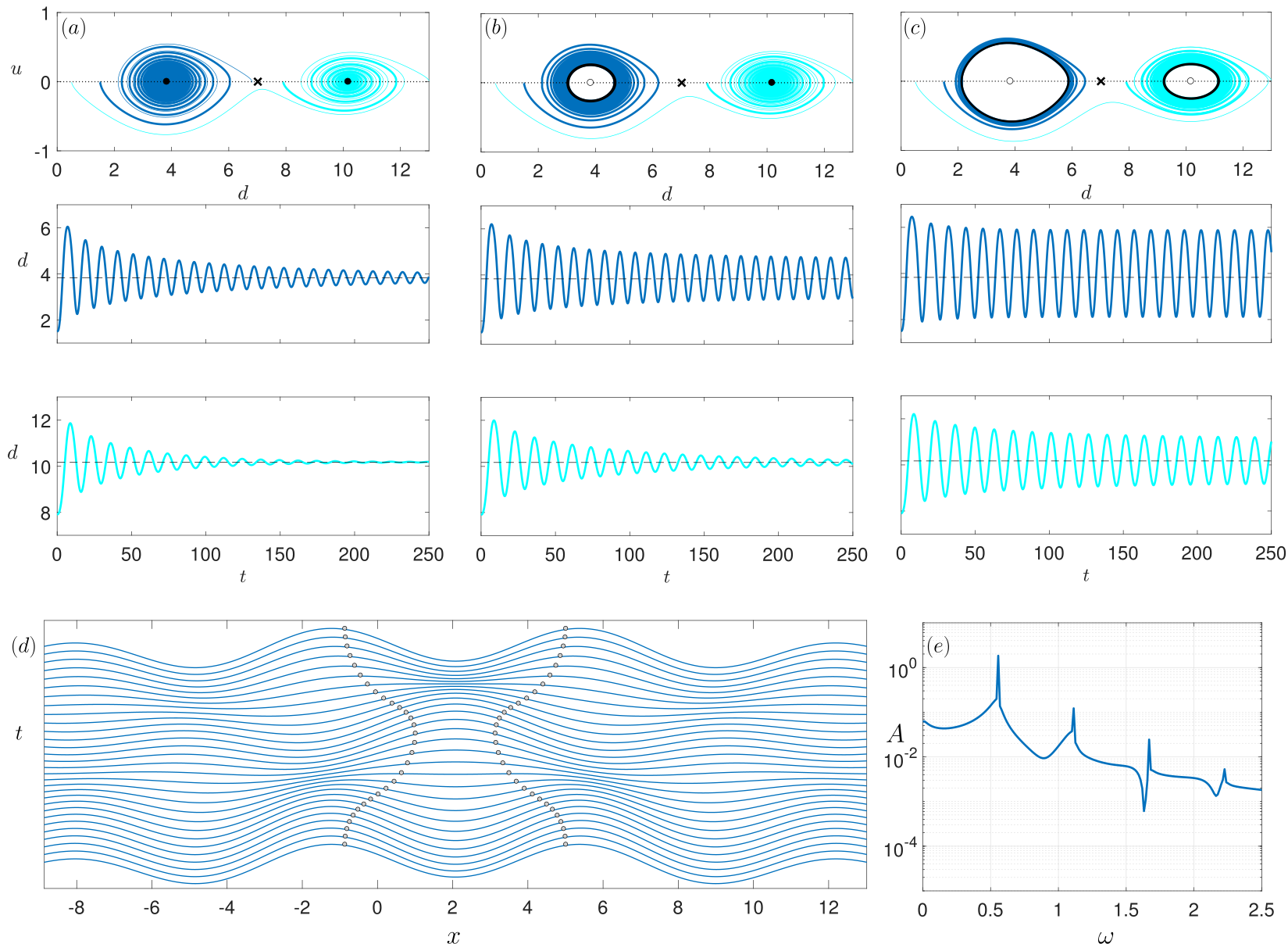
In a sliver of parameter space with inertia exceeding drag, , and small wave forcing , inline oscillations are observed with droplets oscillating towards and away from one another (see Fig. 1). Here we explore the nature of the oscillations.
The phase space for the one-dimensional inline motion of the droplets is two dimensional with the velocity of the first drop and the distance between the droplets sufficient to fully describe the system. The evolution of the phase-space portrait with increasing wave forcing at fixed is shown in Fig. 3. Note that, from equation (6), the value at which different distances with odd become unstable are a function of . For , the cascade of instability goes from larger to smaller distances as increases, while for it goes from smaller to larger distances. For , all the distances become unstable at the same value . For , the onset of inline oscillations occurs at for and for . Thus at (Fig. 3(a)) there are stable spirals at and and a saddle at the unstable distance . If the droplets are perturbed inline when placed near a distance or apart, the oscillations will decay and the droplets will settle back into the stationary distance. As the parameter is increased beyond , the stable spiral at appears to undergo an apparent supercritical Hopf bifurcation and changes into an unstable spiral with an encompassing limit cycle (Fig. 3(b)). Now the droplets either perform limit cycle oscillations corresponding to motion towards and away from one another around or settle into the second stable distance . On further increasing beyond , the stable spiral at also undergoes a supercritical Hopf bifurcation as shown for in Fig. 3(c). Eventually, as is increased beyond , the limit cycle at vanishes in an apparent homoclinic bifurcation, followed by that at at .
In simulations, inline oscillations are observed with rapidly increasing separation as is increased for fixed . The droplets unbind in the simulations when .
Fig. 3(d) shows a representative example of the positions of the droplets along with cross-sections of their wave field for one oscillation cycle. When the droplets are at their maximum separation, the wave field gradient ensures a kick towards each other. As the droplets travel towards each other, they pass their mean distance and reach a minimum separation with wave field gradient such that the droplets receive a kick away from each other. In this way, the droplets oscillate towards and away from one another. Note that the oscillations are dominated by a single frequency (Fig. 3(e)) and a single Fourier mode expansion approximates the oscillations reasonably well near the bifurcation.
VI Parallel walking
For and , a parallel walking state emerges in which the droplets walk at constant speed in the direction perpendicular to the line joining them. Consider two such droplets moving at constant speed and separated by a distance . By substituting and in equation (1), we arrive at the pair of integral equations
and
These can be solved numerically and have infinitely many solutions , for , which are functions of but independent of . The first four such solutions are shown in Fig. 4. Note that droplets in the first and third solutions walk slightly slower than a single droplet while the second and fourth walk slightly faster.
VI.1 Linear stability analysis
To understand the stability of this mode, we use an approach similar to that used by Oza, Rosales, and Bush [2] to explore single droplet walking. The linear stability analysis of parallel walkers with varying phase based on empirical observations has been performed by Arbelaiz, Oza, and Bush [16]. Consider a perturbation to the equilibrium solution and , with the Heaviside step function included to introduce the perturbation at . Substituting this form into equation (1), linearizing and taking Laplace transforms of the resulting equations, we obtain the matrix equation
where
and
where is the identity matrix and
Here
The growth rates of this linear stability problem correspond to the poles of . The functions and decay exponentially as , and so all the functions in the matrix equation above are analytic in the region . Hence finding the growth rates reduces to determining the roots of . This was done using by simultaneously solving real and imaginary parts of using a generalized version of the modified Secant method. We find that the distances and are always unstable while and are stable for a range of and values. Figs. 5(a,b) show the real and imaginary part of the numerically calculated poles as varies for for droplets a distance apart. The first mode to become unstable is a complex conjugate pair indicating an oscillatory mode emerges at the bifurcation. Note that the zero eigenvalue reflects the invariant properties of the base state.
Fig. 5(c) shows the stability diagram for parallel walkers in the - parameter space at a distance apart. The state is stable for a large window of when is small, with the window reducing as the inertia increases. The stable region corresponds well with the region where parallel walkers are observed in simulations, suggesting that the bifurcations away from parallel walking are supercritical.
Note that different modes are the first to become unstable across the two stability curves shown that meet at . For (lower curve), simulations suggest the bifurcation results in oscillating walkers as shown in Fig. 1, while for back-and-forth walkers are observed that often become unbound in simulations.
VII Oscillating walkers
Parallel walkers bifurcate into oscillating walkers, as observed in the parameter space plot in Fig. 1. In this mode, the droplets oscillate towards and away from one another while walking. This state has been observed experimentally.[13, 16]
The first mode to appear has symmetric motion of the droplets relative to the trajectory of their center of mass. In Fig. 6, we plot the numerically simulated trajectory of such walkers, along with the underlying wave field, near the bifurcation from parallel walking. When the droplets are relatively far apart, the wave field of each droplet is discernible. However, when the droplets approach each other, their combined wave field generates a wave barrier. Note that the oscillations are primarily in the inline direction, along the direction between the two droplets, although a small oscillation also appears in the transverse, walking direction. These two components of the oscillations are completely out of phase. As is increased for fixed for these walkers, the amplitude of the oscillations grows until a new, lopsided oscillating mode appears, as described below in Section VII.1.
Oscillating walkers also appear for values immediately above the tongue of unbound states at moderately small and moderately large where inertia is too large for the droplets to be contained by the relatively weak wave field. These are similar in structure to those bifurcating from parallel walkers, except that as increases their amplitude continues to increase, their inertia is sufficient to overcome the central wave barrier and they begin interchanging positions, as described below in Section VII.2.

VII.1 Lopsided walkers
Bifurcations from symmetrically oscillating parallel walkers at moderately small are to an asymmetrically oscillating mode as shown in Fig. 7. These asymmetries can be pronounced as shown, or can be more subtle with standard oscillations that are no longer perpendicular to the direction of motion. In all cases, the center of mass of the two-droplet system now also oscillates. Where these modes are observed, they switch from an initial symmetrically oscillating state. Except at the value where this mode is first observed, this switch is accompanied by an abrupt change in average direction of walking. This abrupt change in direction is a pre-cursor to discrete-turning walkers described in Section VIII.2.


VII.2 Switching walkers
In a tongue of parameter space in the range and , switching walkers are observed. These are symmetrically oscillating walkers whose amplitude is sufficient to result in the droplets interchanging position.
Intertwined regions of periodic and chaotic switching are found as shown in Fig. 8. There are two main types of periodic switching: In the first, the amplitude of oscillations is constant and switching taking place periodically. In the second, the amplitude changes periodically in addition to the switching. Typical trajectories for each type are shown in Figs. 8(a,b). In most of the periodic switching trajectories, the droplets switch after every oscillation (called period- switching) although higher-period switching is also observed.
Switching of droplets also occurs in a chaotic fashion. The chaos can either be just in the amplitude with regular switching or in both the amplitude and the switching of the oscillating walkers as shown in Fig. 8(c,d). Figs. 8(e,f) show the first return map of the maximum distance as a function of for the chaotic trajectories shown. The return map is multi-valued when there is chaos in both amplitude and switching, while it is single valued for the case when there is chaos only in the amplitude. Moreover, the former seems to show hints of stretching and folding similar to a Smale horseshoe map.[20]
We emphasise that such modes are unphysical because the two droplets occupy the same location as they cross their center line. To correct this, the interaction between two nearly touching droplets would need to be included in the governing model. This is beyond our present scope.
VIII Wandering walkers
More exotic behaviors are observed in the simulations once they begin to deviate from on-average straight-line walking. A detailed analysis of these is beyond our scope, but here we describe some of the more interesting dynamical features.
VIII.1 Back-and-forth walkers
These are rare states found for small inertia, , and occur shortly after parallel walkers become unstable. The droplets in these trajectories walk as oscillating walkers but they reverse their direction of walking after several oscillations (Fig. 9). This type of dynamics seems to be unstable and although observed at intermediate times in most of the simulations in this region of parameter space, the droplets usually unbind before the end of the simulation.

VIII.2 Discrete-turning walkers
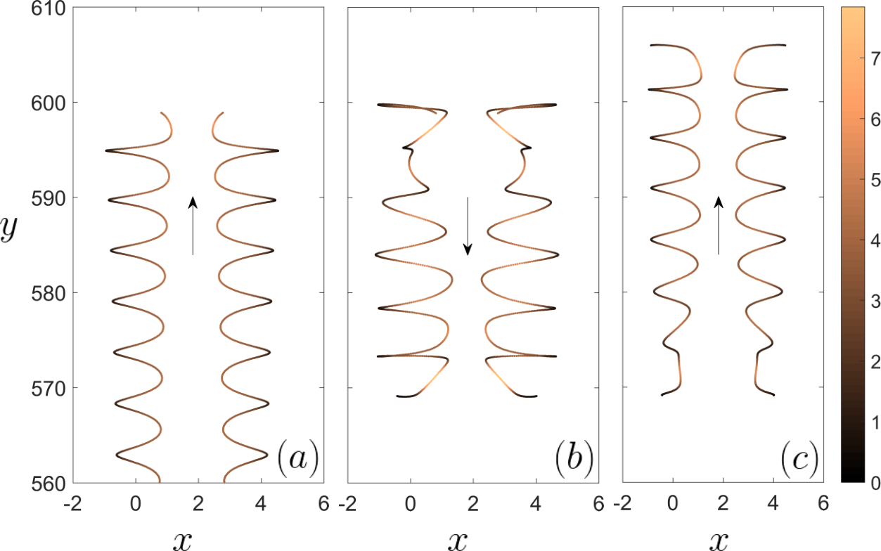
The bifurcations from parallel walkers to (symmetrically) oscillating walkers to lopsided walkers culminate in discrete-turning walkers in a narrow region near and . In this regime, the two droplets perform repeated quantized turns after walking in an on-average straight line for some distance. Fig. 10(a) shows a typical trajectory. In Figs. 10(b,c), we show two phase-space projections illustrating the lead-up to discrete-turning walkers with variables of the distance between the two droplets, the speed of the droplets in the direction of the line joining them and the cosine of the angle between the velocity of the center of mass and the line joining the droplets. Relevant equilibria of the and parallel walking modes and the chasing mode (see Appendix B) are indicated as black filled circles and crosses. In the trajectory shown in Figs. 10(a), the droplets start out as symmetrically oscillating walkers and make multiple discrete turns before settling into a stable lopsided motion. The limit cycle associated with walkers oscillating symmetrically around the equilibrium is shown by the purple curves and the stable lopsided walkers are shown by the navy blue curves. Turns are shown in yellow. When a pair of symmetrically oscillating walkers attempts to transition from the symmetric mode to the lopsided, it gets flung towards the chasing fixed point in the phase space as shown in Fig. 10(c). This fixed point being unstable, brings the droplets back to the symmetrically oscillating walkers mode at . This loop near the chasing fixed point in the phase space corresponds to the actual turn in the trajectory.
As is increased, it appears that the loops towards the chasing mode begin to dominate and the two droplets briefly chase one another before decaying either to the parallel walking fixed point or the fixed point. When it goes to the parallel walking fixed point, it is accompanied by a turn which is nearly right angled and then cascades back to the parallel walking distance as symmetrically oscillating walkers. We call these right-angled discrete turning walkers and they are shown in Fig. 11.
The underlying wave field shows that the turns are due to one of the walkers being reflected from a wave barrier. On studying the statistics of the turning angles, we find a strong peak near (Fig. 11(d)), which is also evident from the trajectories. Nearly right-angle turns are observed for all simulations in this region. At larger scales, the trajectory appears like a random walk (Fig. 11(a)). By calculating the mean squared displacement as a function of time for an ensemble of simulations at and , we find a sub-diffusive exponent of . Such discrete turning behavior has been observed for a single floating water droplet on the surface of a vertically vibrated highly viscous silicone oil bath.[21]

A region of discrete-turning walkers is also observed in a small window at and . These behave similarly, except they tend to walk in straight lines for longer before abruptly turning. A larger region of discrete-turning walkers is observed between and . These are switching walkers and a typical trajectory is shown in Fig. 12(a). Note that in these trajectories, the droplets do not necessarily occupy the same location at the same time.
Discrete-turning walkers are not always stable. When they are unstable, they typically unbind (as indicated in the mixed gray/green region in Fig. 1), although occasionally they cascade into tight orbits. These are reminiscent of cascades from oscillating walkers to orbits that have recently been observed in experiments.[16]
VIII.3 Continuously turning walkers
For larger inertia, these abrupt discrete turns become smoothed, as shown in the progression of trajectories for increasing and fixed in Fig. 12. For sufficiently large inertia, the turns become a series of loops and eventually closed circles. Note that for , the droplets are switching position. Although their trajectories cross, they do not necessarily occupy the same position at the same time.
VIII.4 Closed trajectories and nearly closed trajectories
Remarkably, we find that initially parallel walkers traveling in a straight line can ultimately settle into closed trajectories. Such states are primarily observed at high inertia as indicated by the pink region in the parameter space plot Fig. 1. In this region, the trajectories are circles, as shown in a representative plot in Fig. 12(d).

Circular closed trajectories also appear near and or . In the former region, the droplet mode is a lopsided oscillation as shown in Fig. 13(a), while in the latter it is a symmetric oscillation. Rare regular polygons also appear in isolation in the parameter space, including a hexagon (Fig. 13(c)), an octagon (not shown) and a nonagon (Fig. 13(d)). In the closed-trajectory region near and , smoothed star-shaped trajectories are observed such as the exterior of an enneagram in Fig. 13(b). Polygons shaped orbits have been previously observed for diametrically opposed orbiting walkers[15] but the closed trajectories we observe here are much larger in extent. We note that these polygonal structures are very sensitive to the numerical time step chosen, and we have not been able to reproduce them at smaller time steps although we can reliably reproduce them with different initial conditions. We think this is because the parameters at which they form change slightly with the modified time step and we have not been able to find the exact values at which they reappear.
Intriguingly, in all closed trajectories, only the waves from the previous two oscillations of the droplets have not decayed to less than a tenth of their initial value (estimated from the location of the droplets two units of time earlier, where the exponential decay of the amplitude is ). In particular for the polygonal paths, this suggests that the waves from the previous turn are not directly contributing to the next turn. However, a “memory” of the previous turn is retained by the system as shown in Fig. 13(e): the droplets are not walking symmetrically with the inner droplet on a turn leading its partner along the edges.
IX Conclusions
In this paper, we have taken the Oza–Rosales–Bush stroboscopic walking-droplet model[10] as a theoretical pilot-wave description and explored the remarkable range of possible behaviors for a pair of droplets initially walking in parallel. With increasing inertia and/or wave forcing , the droplets’ motion gains degrees of freedom, commencing from a stationary pair where drag dominates both inertia and wave forcing. The droplets first gain a single translational degree of freedom, either oscillating in place for larger or parallel walking at constant speed and constant separation for larger . For larger and moderate , both modes are apparent and the droplets oscillate towards and away from one another with their center of mass moving in a straight line. For larger still, the droplets perform this motion with random changes in direction by before gaining an additional degree of freedom with increased by taking discrete turns of less than while walking. With sufficient inertia, these turns eventually become continuous. Surprisingly, we find that droplets only unbind if the wave forcing is large and inertia is moderately small or in a narrow tongue where is small and moderately large. For large and , the states observed at long times are intriguing: closed trajectories with effective diameters many tens of Faraday wavelengths and many times the wavelengths of the droplets’ oscillations towards and away from one another. These closed trajectories can be either regular polygons or circles.
Our investigation has reproduced all states that have been observed experimentally: inline oscillations, parallel walkers and symmetrically oscillating walkers (promenading pairs).[13, 16] Our simulations agree quantitatively with where oscillating walkers have been observed (white curve in Fig. 1) except at the highest memories. Parameters for existing experimental setups are restricted to a wedge of parameter space between the white dashed curves in Fig. 1. Besides the experimentally observed states, we predict switching modes, discrete-turning walkers and closed circular trajectories in this region. Switching walkers are unlikely to be observed in the form described here and the droplets might either bounce off one-another, coalesce, or possibly continue walking as a condensed pair. The important facet of an evolving impact phase in experiments may modify or even suppress any turning mode. It would be interesting to explore whether any of the behaviors are realized.
Our investigation has focused on modes derived from parallel walkers. Another fundamental mode is chasers, where the droplets walk one behind the other in a straight line at constant speed. These are not observed in the parameter space of Fig. 1 and the linear stability results of Section IV suggest that parallel walking and inline modes dominate chasing. Durey and Milewski [22] presented a brief study of droplet trains in their model incorporating the vertical dynamics and found that two-droplet trains (equivalent to chasers) are unstable for identical, in-phase droplets with general perturbations but can become stable for out-of-phase droplets. We briefly explore the stability of the chasing mode for in-phase droplets using the stroboscopic model in Appendix B.
Acknowledgements.
We are grateful to John Bush, Andy Hammerlindl, Joel Miller, and Tapio Simula for useful discussions. This research was partially funded by an Australian Government Research Training Program (RTP) Scholarship to R.V.Appendix A Numerical Method
We solve the trajectory equations presented in (1) using a modified Euler method. For , the droplets are assumed to be in a parallel walking state with and . The new position of the droplet is calculated form the old position using a forward Euler step as follows:
To calculate the new velocity, we use the updated position and use a backward Euler step as follows,
| (7) |
| (8) |
where,
| (9) |
| (10) |
The integral in equations (7) and (8) were performed using trapezoidal rule where we consider the contribution from all the previous impacts for the first 1280 timesteps ( using ) and then the contribution from the last 1280 impacts for . At 1280 previous impacts, the exponential damping factor has reached so we neglect all the contribution from impacts beyond 1280 previous steps. The integral for initial condition in equations (9) and (10) were calculated using an adaptive Gauss-Kronrod quadrature routine built into MATLAB. The convergence of this method for the parallel walking solution is shown in Fig. 15.
Using our method, we have been able to reproduce the exotic trajectories of a single walker in a rotating frame by Tambasco et al. [23] and Oza et al. [10]
Fig. 14 shows the comparison with different timesteps of the closed circular trajectory at and where the pair of walkers are in a lopsided mode and the right-angled discrete turning walkers at and . Simulating trajectories at this parameter value with timesteps , and with noise in initial conditions confirm that these exotic behaviours are robust.
Appendix B Chasing mode
Consider two in-phase droplets chasing one another in one-dimensional motion at a constant speed and maintaining a constant separation : and . Substituting these forms into (1), we obtain the following pair of equations:
| (11) |
Here the first integral represents the force on the droplet due to its own wave field while the second integral is the force from the other droplet’s wave field.
Fig. 16 shows the numerical solutions of (11) as a function of (solutions are independent of ). There are infinitely many solution pairs and . Each solution pair only exists for a window of values. The solution first emerges from the corresponding stationary state solution at with and . Pairs of solution pairs coincide and annihilate one another in a saddle-node bifurcation at the upper end of the window.
B.1 Linear stability analysis
To understand the stability of this mode, we consider a general perturbation to a pair of droplets in the chasing mode applied at as follows: and , similar to the analysis for parallel walkers. Substituting this form into (1) and linearising, we find
for , with the negative signs, and , with the positive signs. On taking Laplace transforms on both sides, the equations can be rewritten in the matrix form
where
and
Here are the dynamical variables in the time domain and are the dynamical variable in Laplace space and
with
where is the Laplace transform operator. Fig. 17(a) and (b) shows the real Re and imaginary Im part of the poles of as a function of for chasing walkers at distance and with . Note that the zero eigenvalue reflects the invariant properties of the base state. There is always a transverse mode with Re for both and indicating that the chasers are always unstable for general perturbations. This hold true for all . For , we see that the only unstable mode (complex conjugate) corresponding to the inline perturbation crosses Re around indicating that droplets are stable to inline perturbations for , where is where the chasing solution terminates. A stability diagram in the - parameter space indicating the stable and unstable region to inline perturbations at is shown in Fig. 17(c).
References
References
- [1] Y. Couder, E. Fort, C.-H. Gautier, and A. Boudaoud, Physical review letters 94, 177801 (2005).
- [2] A. U. Oza, R. R. Rosales, and J. W. Bush, Journal of Fluid Mechanics 737, 552 (2013).
- [3] Y. Couder and E. Fort, Physical review letters 97, 154101 (2006).
- [4] A. U. Oza, D. M. Harris, R. R. Rosales, and J. W. Bush, Journal of Fluid Mechanics 744, 404 (2014a).
- [5] S. Perrard, M. Labousse, M. Miskin, E. Fort, and Y. Couder, 5, 3219 EP (2014a), article.
- [6] S. Perrard, M. Labousse, E. Fort, and Y. Couder, Phys. Rev. Lett. 113, 104101 (2014b).
- [7] D. M. Harris, J. Moukhtar, E. Fort, Y. Couder, and J. W. M. Bush, Phys. Rev. E 88, 011001 (2013).
- [8] P. J. Sáenz, T. Cristea-Platon, and J. W. M. Bush, Nature Physics (2017), 10.1038/s41567-017-0003-x.
- [9] A. Eddi, E. Fort, F. Moisy, and Y. Couder, Physical review letters 102, 240401 (2009).
- [10] A. U. Oza, Ø. Wind-Willassen, D. M. Harris, R. R. Rosales, and J. W. Bush, Physics of Fluids 26, 082101 (2014b).
- [11] K. M. Kurianski, A. U. Oza, and J. W. M. Bush, Phys. Rev. Fluids 2, 113602 (2017).
- [12] S. Protière, A. Boudaoud, and Y. Couder, Journal of Fluid Mechanics 554, 85 (2006a).
- [13] C. Borghesi, J. Moukhtar, M. Labousse, A. Eddi, E. Fort, and Y. Couder, Physical Review E 90, 063017 (2014).
- [14] S. Protière, S. Bohn, and Y. Couder, Phys. Rev. E 78, 036204 (2008).
- [15] A. U. Oza, E. Siéfert, D. M. Harris, J. Moláček, and J. W. Bush, Physical Review Fluids 2, 053601 (2017).
- [16] J. Arbelaiz, A. U. Oza, and J. W. M. Bush, Phys. Rev. Fluids 3, 013604 (2018).
- [17] P. A. Milewski, C. A. Galeano-Rios, A. Nachbin, and J. W. Bush, Journal of Fluid Mechanics 778, 361 (2015).
- [18] R. N. Valani, A. C. Slim, and T. Simula, (Under Review) (2018).
- [19] S. Protière, A. Boudaoud, and Y. Couder, Journal of Fluid Mechanics 554, 85–108 (2006b).
- [20] J. Guckenheimer and P. Holmes, Nonlinear oscillations, dynamical systems, and bifurcations of vector fields, Vol. 42 (Springer Science & Business Media, 2013).
- [21] H. Ebata and M. Sano, Scientific Reports 5, 8546 EP (2015), article.
- [22] M. Durey and P. A. Milewski, Journal of Fluid Mechanics 821, 296–329 (2017).
- [23] L. D. Tambasco, D. M. Harris, A. U. Oza, R. R. Rosales, and J. W. M. Bush, Chaos: An Interdisciplinary Journal of Nonlinear Science 26, 103107 (2016).