Embodying probabilistic inference in biochemical circuits

Probabilistic models have been used to capture many features of dynamic and uncertain environments. One of the simplest probabilistic models for modeling change is the discrete-time, finite-state Markov model. In this model, it is assumed that the state of the environment at time $t$ is dependent only on the prior states going back to the $t-k$ time point, where $k$ is the order of the model (when $k=1$, we have a first-order Markov model). While this Markov assumption is violated by many natural processes (Yu,, 2010), it can still serve as a useful idealization (or null model) in some contexts. We chose to focus on this simple model in order to better understand how biochemical circuits that perform inference can be systematically derived from a probabilistic model’s description.

For simplicity, we consider a changing environment that can be in one of only two states, $A$ or $B$, and in which switches between states are driven by a first-order Markov model in discrete time. Such models are parameterized by two transition probabilities: the probability of switching from $A$ to $B$, denoted $\pi_{AB}$, and the probability of switching from $B$ to $A$, $\pi_{BA}$—as shown in Fig. 1A. This model produces sequences of $A$s and $B$s that can be used to generate perturbations in a chemical environment (e.g., a bioreactor containing microbes where nutrients are flowed in and out). We used these sequences to add/remove $A$ or $B$ at fixed time intervals using the following procedure. At first, a state $X_{0}\in\{A,B\}$ is sampled from the Markov model and then a fixed amount of $X_{0}$ is added to a reactor which contains our circuit but has no $A$ or $B$ in it. We assume that $A$ and $B$, which can be thought of as nutrients, are degraded by the circuit at some constant rate. After a fixed time interval, we sample $X_{t+1}$ from the model given the previous state $X_{t}$. If $X_{t+1}=X_{t}$, no perturbation is performed, and if $X_{t+1}\neq X_{t}$, we remove all $A$ and $B$ present in the reactor and add $X_{t+1}$. An environment generated by this procedure using a Markov model where $\pi_{AB}=\pi_{BA}=0.95$ is shown in Fig. 1B.

Assuming the environment’s perturbations are generated by a Markov model, probabilistic inference can be used to anticipate the environment’s future states. In particular, it is useful to compute the probability of encountering $A$ or $B$ next, given past observations of the environment’s states, $\mathsf{history}=\left<X_{t},X_{t-1},X_{t-2},\dots\right>$, where $X_{t}$ corresponds to the state of the environment at time $t$. In Bayesian terms, anticipation of the environment often means computing the posterior predictive distribution, $P(X_{t+1}\mid\mathsf{history})$. This computation is complicated by the fact that the transition probabilities $\pi_{AB}$ and $\pi_{BA}$ are unknown. The standard strategy in such cases is to place prior probabilities on these parameters and then integrate them out to calculate, $\int P(X_{t+1}\mid\mathsf{history},\pi_{AB},\pi_{BA})d\pi_{AB}d\pi_{BA}$. An alternative and sometimes simpler strategy is to estimate the unobserved transition probabilities, $\pi_{AB}$ and $\pi_{BA}$, and use these estimates to anticipate the next state. We can estimate these transition probabilities using Bayesian inference:

If a mathematically convenient prior distribution is chosen for $P(\pi_{AB},\pi_{BA})$, then Eq. 1 can be solved exactly (see Methods). Using the posterior distribution, we can then obtain estimates of the transition probabilities, $\widehat{\pi}_{AB},\widehat{\pi}_{BA}$, and use these to anticipate the next state by sampling $X_{t+1}\sim P(X_{t+1}\mid X_{t},\widehat{\pi}_{AB},\widehat{\pi}_{BA})$:

An important complication (as pointed out in (Katz and Springer,, 2016)) is that organisms act in their environment while it is changing, so the posterior distribution in Eq. 1 must be estimated in real-time. However, in our setting, this computation simplifies considerably. For one, the sequence of observations about the environment, $\mathsf{history}$, does not have to be stored in full, but can instead be compressed into a matrix $T$ of transition counts (Fig. 1C). Assuming $n$ possible states of the environment, $T$ is an $n\times n$ matrix whose $i$th row indicates the number of times the environment switched from the $i$th state to each of the states. Each row can be further compressed: since the sum of the $i$th row must equal the total number of transitions from state $i$ that have been observed, the matrix can be summarized by $n^{2}-n$ entries. In an environment with two states ($A$ or $B$ in our case), the sufficient statistics are therefore two counts: the number of times the environment switched from $A$ to $B$, and from $B$ to $A$ (see Methods for details).

Using these counts as the representation, an elegant algorithm for computing the posterior distribution in real-time emerges. As the environment changes, update the relevant counts in $T$. Then anticipate the next state given the current state $i$ by: (1) normalizing the $i$th row of $T$ to convert counts into probabilities, and (2) sampling a state from that row. This algorithm relies on several computational operations. First, it is necessary to update the counts by a transition update operation (Fig. 1D) that distinguishes $A\rightarrow B$ transitions from $B\rightarrow A$ transitions. Second, in order to use these counts in downstream computations, we need to be able to convert the counts into probabilities by normalization and sample from the resulting distribution; this can be done via the normalization-sampling operation (Fig. 1E). With these three ingredients—a representation of transition counts in the form of $T$, a transition update operation that operates on $T$, and a way to normalize and sample from a row of $T$—the posterior distribution can be used in real-time.

To implement probabilistic inference for the model shown in Fig. 1, we need to construct a biochemical circuit that performs the computational operations outlined in the previous section. Such a circuit would need a representation of the transition matrix $T$, which is used to record the number of switches between relevant states of the environment. Two operations on $T$ would then need to be realized molecularly: (1) the ability to count directionally, i.e., to record when the environment has switched from state $A$ to $B$ (as opposed to from $B$ to $A$) and store this information in $T$, and (2) the ability to reference a row in $T$, normalize it, and sample from the resulting probability distribution (Fig. 1).

The counts matrix and its associated operations can be implemented using the scheme shown in Fig. 2A. Directional counting requires counting a potentially unbounded number of switches in the environment. One approach is to count such transitions using digital counters proposed in the synthetic biology literature, such as (Friedland et al.,, 2009), but this counter’s capacity is fixed and scales with the number of genetic components in the circuit—making it unsuitable for our purpose. We instead represent the number of transitions using abundances. In this scheme, each of the different states ($A$ or $B$) has a dedicated sensor that, at any given point in time, can sense the presence of $A$ or $B$. The environmental states $A$ and $B$ here can be thought of as ligands (e.g., nutrients) that are sensed by receptors (e.g., on the cell’s surface). The transition update operation on $T$ can be realized as follows. When bound by $A$, the $A$-sensor triggers the production of another molecule, a recorder. In the presence of $B$, the recorder (B-Recorder) triggers the production of a stable memory molecule, A-To-B, whose abundance encodes the number of times an $A\rightarrow B$ transition has occurred (Fig. 2A, left). In effect, the presence of $A$ “prepares” the system to record the presence of $B$ (by producing B-Recorder). This constitutes one arm of the transition update operation. The second arm of the circuit is symmetric, this time starting with $B$. The $B$-sensor triggers the production of another recorder molecule (A-Recorder), the latter causing the production of B-To-A memory molecules (whose concentration encodes the number of $B\rightarrow A$ transitions) (Fig. 2A, right). Note that if we were to examine this counter circuit design as if it were a naturally occurring signaling pathway, it might seem as though it suffers from “crosstalk” between the “$A$ pathway” (which starts with sensing of $A$) and the “$B$ pathway” (which starts with the sensing of $B$). However, this feature is precisely what makes it possible to record the direction of the switch.¹¹ 1 The physiologist H. S. Jennings noted the importance of directional sensing by unicellular organisms in his early study, The Behavior of the Lower Organisms (1906) (Jennings,, 1906). Jennings observed that in response to a variety of environmental changes (such as shifts in temperature or salt concentration), a Paramecium cell’s behavior depends upon the direction of change: “The animal, having been subjected to certain conditions, becomes now subjected to others, and it is the transition from one state to another that is the cause of the reaction. This is a fact of fundamental significance for understanding the behavior of lower organisms. But it is not mere change, taken by itself, that causes the reaction, but change in a certain direction. [emphasis in original.]” (Jennings,, 1906).

The second operation needed for implementing inference is normalization-sampling (Fig. 2B). Normalization-sampling requires accessing a row of $T$ (which contains counts), normalizing its values to obtain probabilities, and then sampling from the resulting probability distribution. On an ordinary digital computer, using a sequential programming paradigm, this is straightforward to implement. A standard algorithm for sampling from a probability vector $\theta$ (in effect, sampling from a multinomial distribution) is: calculate a cumulative sum up to each element $\theta_{i}$, then iterate through $\theta$, draw a uniform random number $w\in[0,1]$ for each entry $\theta_{i}$, and return the first $\theta_{i}$ such that $\sum_{j=1}^{i}\theta_{j}\geq w$. Inside the cell, however, there is no readily accessible notion of sequential iteration to support this procedure; a parallelized mechanism is needed instead.

We can make use of the fact that concentrations lend themselves to encoding probabilities (an idea also used in (Napp and Adams,, 2013)) to derive a non-sequential version of the same computation. Consider two proteins, an Activator and a Repressor, that have expression levels $c_{1}$ and $c_{2}$, respectively (Fig. 2B). We can normalize and sample from the (unnormalized) vector $\theta=[c_{1}\ c_{2}]$ by having the Activator and Repressor bind, in mutually exclusive fashion, a third molecule which we denote Integrator. If Integrator is not in excess of Activator and Repressor, then the fraction of Activator-bound Integrator will be proportional to the concentration of Activator normalized by the sum of concentrations of Activator and Repressor: $\frac{[Act]}{[Act]+[Rep]}$ (Fig. 2B). This means that a molecular interaction that depends on the concentration of Activator-bound Integrator will occur in proportion to the probability $\frac{c_{1}}{c_{1}+c_{2}}$. Note that this does not rely on sequential order; the interactions between Activator, Repressor, and Integrator can all take place in parallel. Normalization of protein abundances in this manner is conceptually similar to the “divisive normalization” operation that has been observed in various neural circuits (Carandini and Heeger,, 2012).

We can put the transition update and normalization-sampling operations together to regulate a gene expression program of interest. For example, a protein associated with the $B$ state, B-Program, can be regulated in a manner proportional to the probability of encountering $B$, as shown in Fig. 2C. In this scheme, memory molecules bind integrators in the presence of $A$ or $B$, and the resulting complex—consisting of memory molecule, integrator and the relevant signal ($A$ or $B$)—can then function to upregulate or inhibit B-Program (Fig. 2C).

This scheme results in a circuit that uses the posterior over transition probabilities to regulate the expression of the environmental state-specific program. Consider the case where the environment is in state $A$. In anticipation of the $B$ state, it is reasonable to set the level of B-Program proportional to the probability of switching from $A$ to $B$, $\pi_{AB}$. The abundance of the A-To-B molecule, which reflects the number of $A\rightarrow B$ switched experienced so far, contains part of this information, but has to be converted into a probability. This is achieved by having the $A$-bound A-To-B memory molecule bind an integrator (shown in black in Fig. 2C), with the resulting complex functioning as an activator that upregulates B-Program. Another molecule, $\textnormal{A-To-B}_{R}$, when $A$-bound, binds to the same integrator site as the $A$-bound A-To-B, turning the complex into a repressor that downregulates B-Program (Fig. 2C). This effectively normalizes A-To-B to produce a probability. In the case when the environment is in state $B$, a symmetric circuit that uses a distinct integrator (shown in grey in Fig. 2C) enacts the same logic using the B-To-A memory molecule.

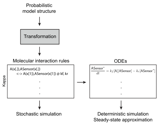
Putting the circuit parts described above together, we can now give a procedure for converting a Markov model into a description of a biochemical circuit that performs inference in this model. We have implemented a computer program (in Python) that, taking advantage of the symmetries in the circuit’s design, generates a description of the circuit in the Kappa language (Danos and Laneve,, 2004; Danos et al.,, 2007). Kappa is a rule-based language describing the direct molecular interactions among proteins and simulating these interactions stochastically (Fig. 3). A rule-based representation is particularly convenient for capturing our circuit, partly because the circuit consists of proteins that play distinct roles depending on the configuration of their binding sites (as in Fig. 2D). While we will focus mainly on stochastic simulation below, Kappa programs can be automatically converted into a set of ODEs that can be used for deterministic simulation and approximation of steady-states (Fig. 3).²² 2 In general, a Kappa program may correspond to an intractably large number of ODEs (due to combinatorial explosion of species (Feret et al.,, 2009)), but this is not an issue for our circuit which has a relatively small number of components and binding sites. The high-level procedure for generating a circuit that performs inference in a Markov model parameterized by a $2\times 2$ transition matrix $T$ is as follows (rate constants omitted for clarity):

1. 1.

   For the first row in $T$: let $X\in\{A,B\}$ and $Y$ be the other state, $Y\in\{A,B\},Y\neq X$.

2. 2.

   Generate rules for transition update:

   1. (a)

      Let X-Sensor be a sensor reversibly activated by $X$: $X+\textnormal{X-Sensor}\xrightleftharpoons{}{\textnormal{X-Sensor}}^{*}$

   2. (b)

      When active, X-Sensor triggers production of Y-Recorder: ${\textnormal{X-Sensor}}^{*}\longrightarrow{\textnormal{X-Sensor}}^{*}+\textnormal{Y-Recorder}$

   3. (c)

      Let Y-Recorder be a recorder reversibly activated by $Y$: $Y+\textnormal{Y-Recorder}\xrightleftharpoons{}{\textnormal{Y-Recorder}}^{*}$

   4. (d)

      When active, Y-Recorder triggers production of X-To-Y memory molecule

3. 3.

   Generate rules for normalization-sampling:

   1. (a)

      Let X-To-Y be reversibly activated by $X$ to form Activator (denoted $Act$): $X+\textnormal{X-To-Y}\xrightleftharpoons{}Act$

   2. (b)

      Let $\textnormal{X-To-Y}_{R}$ be reversibly activated by $X$ to form Repressor (denoted $Rep$): $X+\textnormal{X-To-Y}_{R}\xrightleftharpoons{}Rep$

   3. (c)

      Let Integrator (denoted $Int$) be bound in mutually exclusive fashion by either Activator or Repressor to form the following complexes:

      1. i.

         Activator reversibly binds Integrator to form X-To-Y activation complex, $\textnormal{X-To-Y}_{A}$: $Act+Int\xrightleftharpoons{}\textnormal{X-To-Y}_{A}$

      2. ii.

         Repressor binds Integrator to form X-To-Y repression complex, $\textnormal{X-To-Y}_{R}$: $Rep+Int\xrightleftharpoons{}\textnormal{X-To-Y}_{R}$

4. 4.

   Generate rules for regulating state-specific expression programs³³ 3 Only the rules for B-Program are shown here. Symmetric rules can be generated to regulate A-Program.:

   1. (a)

      $\textnormal{X-To-Y}_{A}$ upregulates B-Program: $\textnormal{X-To-Y}_{A}\longrightarrow\textnormal{X-To-Y}_{A}+\textnormal{B-Program}$

   2. (b)

      $\textnormal{X-To-Y}_{R}$ downregulates B-Program: $\textnormal{X-To-Y}_{A}+\textnormal{B-Program}\longrightarrow\textnormal{X-To-Y}_{A}$

5. 5.

   Repeat above steps for the remaining row of $T$ (i.e., if the above steps were executed with $X=A,Y=B$, now repeat with $X=B,Y=A$).

We generated a Kappa program using this procedure (see Methods for full program). We chose rate constants for various steps (e.g., activation of sensors) that were were biophysically plausible (on par with rates of protein production and post-translational modifications) and assumed that sensors are constitutively expressed. The levels of integrators and repressors were set to be roughly equal. In the next section, we use this program to explore the circuit’s behavior in various changing environments through stochastic simulation.

Inference as embodied in a circuit made of proteins has a number of properties in common with the abstract notion of inference used in our analysis of a Markov model (Fig. 1), but also some important differences. We illustrate these properties below using stochastic simulations of the circuit in different environments.

Properties of an inferential mechanism. The circuit constructed by our procedure has several features that would be expected of a mechanism that learns from its environment’s history. These can be illustrated in an environment that switches periodically from $A$ to $B$ at 50 time-unit intervals, as shown in Fig. 4A. During the initial exposures to switches (time $0-150$, Fig. 4B), there is little to no change in A-Program and B-Program since the memory molecules have not yet accumulated. As the circuit experiences more “data,” an anticipation behavior emerges where B-Program is upregulated ahead of the onset of $B$ (while still in $A$) and A-Program is upregulated in advance of the onset of $B$. Similarly, B-Program begins to be downregulated, in anticipation of $A$, while still in $B$ (and likewise for A-Program).

With more experiences of periodic switches, the strength of the circuit’s anticipatory behavior increases, consistent with the idea that more experiences result in more confident estimates of transition probabilities (mechanistically, this manifests in higher concentrations of memory molecules; Fig. 4B). Furthermore, since slightly more $A\rightarrow B$ switches were experienced than $B\rightarrow A$ switches in this environment (Fig. 4A), the strength of activation for B-Program in the $A$ state is greater than that of the activation of A-Program in the $B$ state. The circuit’s periodic behavior, which roughly matches the 50 time-unit interval of switches in the environment, was not hardcoded in the circuit but rather induced by the pattern of experience. When the periodic pattern of switches in the environment is broken, and $A$ is not followed by $B$, the circuit makes the “wrong” inference and still upregulates B-Program (Fig. 4B, time $1000$). After switching has stopped, the environment’s imprint on the circuit is then “forgotten” as the memory molecules degrade (Fig. 4B, starting at time $1050$).

Coupling of inference and action. Through time, the fraction of activated integrator complexes reflect the posterior over transition probabilities (Fig. 4C). Note that these glimpses of the posterior are only available when the program of interest (A-Program and B-Program) is being regulated. There is no steadily available correlate of the posterior probabilities. We compared this transient “molecular correlate” of the posterior with the estimate of the posterior over the transition probabilities ($\pi_{AB}$ and $\pi_{BA}$) based on a discrete-time two-state Markov model with a uniform prior (treating $A$ and $B$ states as on/off and discretizing the environment into 50 time-unit intervals; Fig. 4D). Like the molecular posterior of the circuit, the idealized estimate of $\pi_{AB}$ and $\pi_{BA}$ increases with time as observations of the environment accumulate (Fig. 4D).

Constraints of embodiment by proteins. The probabilistic model we used to design the circuit was in discrete time, yet cells sense their environment continuously. In the discrete-time model, by contrast, transitions from a state to itself, e.g., $B\rightarrow B$, are recorded assuming a fixed interval of time. Therefore, if $A$ tends to be followed by long sequences of $B$, the estimate of $\pi_{BA}$ should decrease as the count of $B\rightarrow B$ transitions increases (Fig. 5).

The logic of protein production captures this relationship without needing to explicitly posit a fixed time interval. When an $A\rightarrow B$ transition is experienced, the abundance of the A-To-B memory molecule increases. If the environment remains in $B$, then the B-To-A memory molecule, which we assume is degraded at some rate, will decrease in abundance, and $B$ itself will degrade over time as well (Fig. 5A,B). All things being equal, B-To-A will decrease, making way for the repressor $\textnormal{B-To-A}_{R}$ to act. As a consequence, the fraction of active A-To-B Integrator will be greater than the fraction of active B-To-A Integrator (similarly to the idealized posterior, Fig. 5C,D).

Note that the constraints of protein production also limit the abstract probabilistic model we had started out with in other ways. While in the Markov model the “memory” of the environment is determined by the order of the model, here the extent of memory is bounded by the degradation rates of the memory molecules. Without additional mechanisms (such as positive feedback), the circuit’s memory will be effectively limited by the stability of the memory molecules themselves and by dilution (e.g., through cell division).

Variation in coupling inference to action. In designing the circuit, we have not taken into account any special considerations regarding how the state-specific expression programs A-Program and B-Program should behave. It is easy to imagine that different contexts could impose specific constraints on the relationship between the two programs and their kinetics. In some situations, it may be metabolically costly or toxic to have both A-Program and B-Program expressed at the same time. In others, anticipatory regulation of one program may be metabolically cheaper than the other. In the current design, the molecular estimate of the posterior, as realized by the fraction of activated integrators, was used to regulate these programs without tuning the rate constants so as to optimize for any particular constraint. Since continuous variation in rate constants (e.g., those affecting the synthesis and degradation of A-Program and B-Program) can produce many different expression profiles, it is plausible that this aspect of the circuit can be effectively shaped by selective forces.

Relationship to idealized inference. As discussed above, there is not a single quantity that serves as a “molecular correlate” of the posterior stably through time. The closest quantity is the fraction of bound integrators, which is coupled to action as described above. It is nonetheless instructive to compare this correlate more systematically to the idealized posterior. To do this, we simulated changing environments consisting produced using different transition probabilities (Fig. 6). For each environment, we first estimated the median of the posterior over $\pi_{AB}$ at each time point and then took $\widehat{\pi}_{AB}$ to be the median of those estimates (and similarly for $\pi_{BA}$ to get $\widehat{\pi}_{BA}$). We then computed a similar quantity for our circuit by taking the median of the fraction of bound A-To-B integrators through time ($\widehat{I}_{AB}$) and likewise for B-To-A integrators to get $\widehat{I}_{BA}$. Since these quantities are not directly comparable, we compared the ratio of posteriors from the idealized model ($\frac{\widehat{\pi}_{AB}}{\widehat{\pi}_{BA}}$) with the ratio of active integrators in the circuit ($\frac{\widehat{I}_{AB}}{\widehat{I}_{BA}}$). The comparison shows broad agreement between these quantities along different values of transition probabilities (Fig. 6), with the caveat that both quantities are aggregated over time and thus do not capture dynamic differences.

The circuit we have constructed only works when the dynamics of its components are well-matched to the timescales of the environment’s changes. When recorders and sensors are too slow relative to duration of environment switches, for instance, the circuit fails to record the environment’s history (Fig. 7). More subtle modes of failure arise from the circuit’s sensitivity to the abundance, not just the presence, of $A$ and $B$. While in the perturbations presented above we removed all $A$ or $B$ molecules from the environment during each switch, in practice, when the medium in which cells live is altered by an experimenter, only the free (unbound) molecules are removed. When we simulate an environment where only free molecules are removed in each switch, residual $A$ and $B$ molecules accumulate with every switch (Fig. 8). The circuit’s behavior in this case is qualitatively similar to the total perturbations (compare with Fig. 4), but the circuit’s response loses its punctate character (leading to overall higher levels of $A$- and $B$-specific expression programs).

Since the circuit is sensitive to the abundance of the signals and not just to their presence, pulses of varying amplitudes will also affect the levels of the memory molecules. To examine this behavior, we simulated an environment where $A$ additions were twice the size of $B$ additions and only free $A$ or $B$ were removed during switches (Fig. 9). This asymmetry in pulse amplitude results in the circuit having an incorrect representation of the environment’s history. The higher abundance of $A$ results in substantially higher levels of B-To-A relative to A-To-B, yet the number of $A\rightarrow B$ switches is greater than that of $B\rightarrow A$ switches. The resulting representation of the environment is also inconsistent: while $[\textnormal{B-To-A}]\gg[\textnormal{A-To-B}]$, the bigger $A$ pulses—which bind the A-To-B memory molecule—result in the “posterior” of $\pi_{AB}$ (i.e., fraction of activated A-To-B integrator) being consistently greater than the equivalent quantity for $\pi_{BA}$.

We have presented a synthetic design for a circuit that performs inference. But how would one “reverse-engineer” a natural circuit that performed a similarly sophisticated computation? A line of work by neuroscientists and molecular biologists has pointed to cases where measuring input-output relationships of a dynamic and stateful system (whether biological (Marr,, 1982) or synthetic (Mel,, 2000; Lazebnik,, 2002; Jonas and Kording,, 2017)), without a sufficiently detailed theoretical framework in which to interpret these measurements, can lead to potentially misleading descriptions of how the underlying system works. In systems biology, a common approach to studying cellular pathways (enabled in part by high-throughput measurement technologies developed in recent years) has been to quantitatively measure a pathway’s component of interest as a function of a quantitatively varying environmental input. When multiple inputs are varied along a sufficiently large dynamic range, this measurement can reveal surprising relationships between inputs and outputs. For example, (Escalante-Chong et al.,, 2015) measured the level of induction of the galactose metabolic pathway (Gal) in yeast cells grown in different concentrations of glucose (which represses Gal) and galactose (which activates Gal) and found that Gal induction depends on the ratio of glucose to galactose. These experiments are premised on obtaining steady-state-like conditions where the level of the sugars (glucose and galactose) and measured signal are relatively stable.

Could a quantitative approach based on steady-states uncover inference in our circuit? Using the ODE description of our circuit (Fig. 3), we deterministically simulated the circuit across a range of concentrations of the inputs ($A$ and $B$), which were held fixed, and examined the steady-state concentrations of $[\textnormal{B-Program}]$ and the two memory molecules, $[\textnormal{A-To-B}]$ and $[\textnormal{B-To-A}]$ (Fig. 10). The resulting three profiles are broadly similar. The B-Program profile suggests that the circuit is most active when $[A]$ and $[B]$ are both high (and that $B$ must be present for B-Program to be expressed) (Fig. 10A). The steady-state profiles of the memory molecules are also relatively similar to each other across a broad range of input concentrations (Fig. 10B,C).⁴⁴ 4 The relatively small asymmetry between the $[\textnormal{A-To-B}]$ and $[\textnormal{B-To-A}]$ steady-state profiles, which occurs in the higher ranges of $[A]$ and $[B]$, is explained by the fixed level of the sensors (A-Sensor and B-Sensor). Consider the case where $[A]$ and $[B]$ are much higher than the concentrations of the sensors and $[B]\gg[A]$. In this case, $[A]$ will saturate the A-Sensor molecules, resulting in (at most) all of them being active. The activated sensors will then produce a potentially unbounded number of B-Recorder molecules. Since $[B]\gg[A]$, the higher $[B]$ is, the more it can activate the pool of recorders to trigger production of A-To-B. Therefore, when $[B]>[A]$, we expect $[\textnormal{A-To-B}]>[\textnormal{B-To-A}]$. These measurements suggest that the memory molecules are induced in proportion to $[A]$ and $[B]$, masking the fact that each molecule’s concentration encodes a distinct direction of environmental change. This indicates that a standard steady-state analysis, even if performed quantitatively, can obscure the logic underlying a circuit that responds to the environment’s history.

These observations suggest that it would be difficult to interpret the circuit without having a theory about what it does. But what if we did assume that this circuit performs probabilistic inference? Much work by cognitive scientists and neuroscientists has used probabilistic inference as a framework for explaining behavior, which prompted a search for the correlates of these models in biological signals (see the growing “Bayesian brain” literature, e.g., (Knill and Pouget,, 2004)). Given the explanatory power of these models with respect to behavior, it may seem reasonable to look for the molecular signatures and associated “knobs” that correspond to the components of probabilistic models, including the prior, the likelihood function and the posterior. There are at least two conceptual difficulties that arise in this pursuit that can be seen through the analysis of our circuit. First, while inference about (or perception of) the environment is typically separated from “action” in these computational models, in our circuit the two are intimately coupled. As the time-dependent profiles of the circuit show, the closest thing to a “molecular correlate” of a posterior-like quantity—the fraction of activated integrators—only comes into being through action (regulation of a gene expression program such as A-Program and B-Program). There is no stable quantity that serves as a correlate of the posterior through time.

A second difficulty with searching for the molecular basis of inference is that the abstract components of the model may not map neatly onto corresponding molecular knobs. Consider for instance the question of where in the circuit the “prior” lies. One way to conceive of the prior is as the propensity to change one’s prior belief from an initial state of having seen “no data” to another belief state. Technically, the notion of an initial state is artificial here since cells are continuously living inside their environment and sensing its fluctuations. Setting this aside, if we assume that cells start from some initial state (where $A$ and $B$ are absent) then the propensity to change can depend on, among other things, the initial concentration of the repressor molecules. An alternative way to conceive of a “prior” here is as the amount of change in the representation of the environment based on observation of change; i.e., how much does influence one transition has on the internal representation, such as our memory molecules. This notion of “prior” can also be shaped by multiple overlapping and not necessarily modular features, such as the rate constants governing the interaction between the sensors, recorders and memory molecules. This step can also be affected at the layer of “action,” for instance by tweaking how sensitive the state-specific proteins A-Program and B-Program are to change in the levels of memory molecules. Although the circuit is not a soup where all components are enmeshed with all others, there still is not a clear knob one can use to directly and selectively tune “the prior.”

We briefly derive a real-time procedure for inference in a Markov model (which was used to generate the analytic estimate of the posterior in all figures). We assume a first-order discrete-time Markov model over two discrete states, $A$ and $B$, which is characterized by transition probabilities $\pi_{AB}$ and $\pi_{BA}$ (where $\pi_{AA}=1-\pi_{AB}$ and $\pi_{BB}=1-\pi_{BA}$). A sequence of observations is generated from the model by first sampling an initial state $X_{0}$ (from a uniform prior over $A$ and $B$) and sampling subsequent observations $X_{1},X_{2},X_{3},\dots$ using the transition probabilities:

• •

  If $X_{t}=A$, sample $X_{t+1}\sim\mathrm{Bern}(1-\pi_{AB})$

• •

  Otherwise, if $X_{t}=B$, sample $X_{t+1}\sim\mathrm{Bern}(\pi_{BA})$.

A convenient choice of prior over transition probabilities is the Beta distribution. A Beta distribution, $\mathrm{Beta}(\theta;\alpha_{0},\alpha_{1})$, over $\theta\in[0,1]$ is determined by a pair of shape parameters $\alpha_{0},\alpha_{1}$. Different settings of the alphas can be used to encode distinct beliefs about $\theta$. As examples: $\alpha_{0}=\alpha_{1}=1$ is equivalent to a uniform distribution over $[0,1]$, $\alpha_{0}=\alpha_{1}=100$ is a unimodal distribution whose mode is at $\theta=0.5$, and $\alpha_{0}<1,\alpha_{1}<1$ (e.g., $\alpha_{0}=\alpha_{1}=0.5$) is a U-shaped distribution corresponding to the belief that $\theta$ is likely to be close to 0 or 1. The Beta distribution is conjugate to the binomial distribution (Gelman et al.,, 1995), meaning that a posterior that is the product of a Beta prior and a binomial likelihood equals another Beta distribution whose parameters can be calculated exactly.

The observations of the environment, $\mathsf{history}$, can be compressed into as a set of counts (as described in main text) that are binomially distributed, which allows us to use the Beta-Binomial conjugacy to calculate our posteriors of interest analytically. For a two-state Markov model, the relevant counts are: (1) $c_{AB}$, the number of $A\rightarrow B$ transitions, (2) the number of $B\rightarrow A$ transitions, and (3) the number of total switches $s$ in $\mathsf{history}$. (Note that the other entries of the transition counts matrix $T$ can be computed from this pair of summary statistics and $s$: $c_{AA}=s-c_{AB}$ and $c_{BB}=s-c_{BA}$.) We can then expand the posterior over $\pi_{AB}$ as follows:

This posterior can be computed in real-time up through the $k$th observation (a task which is called “filtering” (Särkkä,, 2013)) using a recursive procedure that proceeds as follows. Let $C^{k}_{AB}$ be the number of $A\rightarrow B$ transitions up to the $k$th observation, and let $b^{k}_{\pi_{AB}}$ be the posterior up to the $k$th observation. The base case of the procedure is the first observation, which is the switch from $X_{0}\rightarrow X_{1}$ (where $k=1$):

We can now define the $b^{k+1}_{\pi_{AB}}$ in terms of $b^{k}_{\pi_{AB}}$ by noting that the posterior as of the $k$th observation, $b^{k}_{\pi_{AB}}$, serves as the prior at $k+1$. Let $\alpha^{k}_{0},\alpha^{k}_{1}$ be the parameters of $b^{k}_{\pi_{AB}}$. Now let $I_{AB}$ be an indicator variable that is 1 if $X_{k}\rightarrow X_{k+1}$ is an $A\rightarrow B$ transition (and 0 otherwise), and $I_{AA}$ an indicator variable that is 1 if $X_{k}\rightarrow X_{k+1}$ is an $A\rightarrow A$ transition (and 0 otherwise). Then the posterior after the $k+1$ observation is:

Note that if $X_{k}=B$, then $I_{AB}=I_{AA}=0$, which means the estimate of the posterior over $\pi_{AB}$ does not change (i.e., $b^{k+1}_{AB}=b^{k}_{AB}$). The same derivation as above applies to the posterior over $\pi_{BA}$.

To estimate the posterior over the transition probabilities in the above figures (e.g., Fig. 4D), we used the median of the posterior distribution at each time step.

Stochastic simulations were performed using Kappa’s KaSim (version: v4.0rc1-155-g93b4c2f). ODEs (in SBML format) corresponding to the Kappa program were generated using the KaDE utility (Camporesi et al.,, 2017) and simulated using the roadrunner library in Python (Somogyi et al.,, 2015). For steady-state simulations in the presence of fixed inputs (Fig. 10), we ran the ODE simulation until the sum of changes (across all species) between time bins was less than a fixed threshold ($0.001$).

• •

  Programmatically generated Kappa program corresponding to two-state inference circuit.

• •

  ODEs corresponding to circuit (in SBML format) generated by KaDE.

References

- Adam, (2006) Adam, A. (2006). Artificial knowing: Gender and the thinking machine. Routledge.
- Balázsi et al., (2011) Balázsi, G., van Oudenaarden, A., and Collins, J. J. (2011). Cellular decision making and biological noise: from microbes to mammals. Cell, 144(6):910–925.
- Baluška and Levin, (2016) Baluška, F. and Levin, M. (2016). On having no head: cognition throughout biological systems. Frontiers in Psychology, 7:902.
- Bray, (1990) Bray, D. (1990). Intracellular signalling as a parallel distributed process. Journal of Theoretical Biology, 143(2):215–231.
- Camporesi et al., (2017) Camporesi, F., Feret, J., and Lỳ, K. Q. (2017). KaDE: A Tool to Compile Kappa Rules into (Reduced) ODE Models. In International Conference on Computational Methods in Systems Biology, pages 291–299. Springer.
- Carandini and Heeger, (2012) Carandini, M. and Heeger, D. J. (2012). Normalization as a canonical neural computation. Nature Reviews Neuroscience, 13(1):51.
- Danos et al., (2007) Danos, V., Feret, J., Fontana, W., and Krivine, J. (2007). Scalable simulation of cellular signaling networks. In Shao, Z., editor, Programming Languages and Systems, 5th Asian Symposium, APLAS 2007, Singapore, November 29-December 1, 2007, Proceedings, volume 4807 of Lecture Notes in Computer Science, pages 139–157. Springer.
- Danos and Laneve, (2004) Danos, V. and Laneve, C. (2004). Formal molecular biology. Theoretical Computer Science, 325(1):69–110.
- Escalante-Chong et al., (2015) Escalante-Chong, R., Savir, Y., Carroll, S. M., Ingraham, J. B., Wang, J., Marx, C. J., and Springer, M. (2015). Galactose metabolic genes in yeast respond to a ratio of galactose and glucose. Proc. Natl. Acad. Sci. U.S.A., 112(5):1636–1641.
- Fages et al., (2017) Fages, F., Guludec, G. L., Bournez, O., and Pouly, A. (2017). Strong turing completeness of continuous chemical reaction networks and compilation of mixed analog-digital programs. In Feret, J. and Koeppl, H., editors, Computational Methods in Systems Biology - 15th International Conference, CMSB 2017, Darmstadt, Germany, September 27-29, 2017, Proceedings, volume 10545 of Lecture Notes in Computer Science, pages 108–127. Springer.
- Feret et al., (2009) Feret, J., Danos, V., Krivine, J., Harmer, R., and Fontana, W. (2009). Internal coarse-graining of molecular systems. Proceedings of the National Academy of Sciences, 106(16):6453–6458.
- Fernando et al., (2009) Fernando, C. T., Liekens, A. M., Bingle, L. E., Beck, C., Lenser, T., Stekel, D. J., and Rowe, J. E. (2009). Molecular circuits for associative learning in single-celled organisms. Journal of the Royal Society Interface, 6(34):463–469.
- Friedland et al., (2009) Friedland, A. E., Lu, T. K., Wang, X., Shi, D., Church, G., and Collins, J. J. (2009). Synthetic gene networks that count. science, 324(5931):1199–1202.
- Gallistel, (2008) Gallistel, C. R. (2008). Learning and representation. In Menzel, R. and Byrne, J., editors, Learning and Memory: A Comprehensive Reference. Elsevier.
- Gallistel and Matzel, (2013) Gallistel, C. R. and Matzel, L. D. (2013). The neuroscience of learning: beyond the hebbian synapse. Annual Review of Psychology, 64:169–200.
- Gelman et al., (1995) Gelman, A., Carlin, J. B., Stern, H. S., and Rubin, D. B. (1995). Bayesian Data Analysis. Chapman and Hall, London.
- Griffiths et al., (2010) Griffiths, T. L., Chater, N., Kemp, C., Perfors, A., and Tenenbaum, J. B. (2010). Probabilistic models of cognition: Exploring representations and inductive biases. Trends in cognitive sciences, 14(8):357–364.
- Hjelmfelt et al., (1991) Hjelmfelt, A., Weinberger, E. D., and Ross, J. (1991). Chemical implementation of neural networks and turing machines. Proceedings of the National Academy of Sciences, 88(24):10983–10987.
- Jablonka and Raz, (2009) Jablonka, E. and Raz, G. (2009). Transgenerational epigenetic inheritance: prevalence, mechanisms, and implications for the study of heredity and evolution. The Quarterly review of biology, 84(2):131–176.
- Jacob et al., (2004) Jacob, E. B., Becker, I., Shapira, Y., and Levine, H. (2004). Bacterial linguistic communication and social intelligence. Trends in Microbiology, 12(8):366–372.
- Jennings, (1906) Jennings, H. S. (1906). Behavior of the Lower Organisms, volume 10. Columbia University Press, The Macmillan Company.
- Jonas and Kording, (2017) Jonas, E. M. and Kording, K. P. (2017). Could a neuroscientist understand a microprocessor? PLoS Computational Biology, 13(1):e1005268.
- Katz and Springer, (2016) Katz, Y. and Springer, M. (2016). Probabilistic adaptation in changing microbial environments. PeerJ, 4:e2716.
- Knill and Pouget, (2004) Knill, D. C. and Pouget, A. (2004). The bayesian brain: the role of uncertainty in neural coding and computation. Trends in Neurosciences, 27(12):712–719.
- Lake et al., (2017) Lake, B. M., Ullman, T. D., Tenenbaum, J. B., and Gershman, S. J. (2017). Building machines that learn and think like people. Behavioral and Brain Sciences, 40.
- Lambert and Kussell, (2014) Lambert, G. and Kussell, E. (2014). Memory and Fitness Optimization of Bacteria under Fluctuating Environments. PLoS Genetics, 10(9):e1004556.
- Lazebnik, (2002) Lazebnik, Y. (2002). Can a biologist fix a radio? Or, what I learned while studying apoptosis. Cancer Cell, 2(3):179–182.
- Lyon, (2015) Lyon, P. (2015). The cognitive cell: bacterial behavior reconsidered. Frontiers in microbiology, 6:264.
- Marr, (1982) Marr, D. (1982). Vision: A computational investigation into the human representation and processing of visual information. New York: WH Freeman.
- Maturana and Varela, (1980) Maturana, H. and Varela, F. (1980). Autopoiesis and Cognition: The Realization of the Living. Boston studies in the philosophy of science. D. Reidel.
- Maturana, (1978) Maturana, H. R. (1978). Cognition. In Hejl, P. M., Köck, W. K., and Roth, G., editors, Wahrnehmung und Kommunikation, pages 2247–2255. Lang.
- Maturana and Varela, (1987) Maturana, H. R. and Varela, F. J. (1987). The tree of knowledge: The biological roots of human understanding. New Science Library/Shambhala Publications.
- McGregor et al., (2012) McGregor, S., Vasas, V., Husbands, P., and Fernando, C. (2012). Evolution of associative learning in chemical networks. PLoS computational biology, 8(11):e1002739.
- Mel, (2000) Mel, B. W. (2000). In the brain, the model is the goal. Nature Neuroscience, 3:1183–1183.
- Merleau-Ponty, (1964) Merleau-Ponty, M. (1964). Eye and Mind. In Edie, J. and Cobb, W., editors, The Primacy of Perception: And Other Essays on Phenomenological Psychology, the Philosophy of Art, History, and Politics. Northwestern University Press.
- Mitchell et al., (2009) Mitchell, A., Romano, G. H., Groisman, B., Yona, A., Dekel, E., Kupiec, M., Dahan, O., and Pilpel, Y. (2009). Adaptive prediction of environmental changes by microorganisms. Nature, 460(7252):220–224.
- Napp and Adams, (2013) Napp, N. E. and Adams, R. P. (2013). Message passing inference with chemical reaction networks. In Burges, C. J. C., Bottou, L., Welling, M., Ghahramani, Z., and Weinberger, K. Q., editors, Advances in Neural Information Processing Systems 26, pages 2247–2255. Curran Associates, Inc.
- Raj and van Oudenaarden, (2008) Raj, A. and van Oudenaarden, A. (2008). Nature, nurture, or chance: stochastic gene expression and its consequences. Cell, 135(2):216–226.
- Särkkä, (2013) Särkkä, S. (2013). Bayesian Filtering and Smoothing. Cambridge University Press, New York, NY, USA.
- Smolensky, (1986) Smolensky, P. (1986). Information processing in dynamical systems: Foundations of harmony theory. Technical report, University of Colorado Computer Science Department.
- Soloveichik et al., (2010) Soloveichik, D., Seelig, G., and Winfree, E. (2010). Dna as a universal substrate for chemical kinetics. Proceedings of the National Academy of Sciences, 107(12):5393–5398.
- Somogyi et al., (2015) Somogyi, E. T., Bouteiller, J.-M., Glazier, J. A., König, M., Medley, J. K., Swat, M. H., and Sauro, H. M. (2015). libRoadRunner: a high performance SBML simulation and analysis library. Bioinformatics, 31(20):3315–3321.
- Stockwell et al., (2015) Stockwell, S. R., Landry, C. R., and Rifkin, S. A. (2015). The yeast galactose network as a quantitative model for cellular memory. Molecular bioSystems, 11(1):28–37.
- Tagkopoulos et al., (2008) Tagkopoulos, I., Liu, Y. C., and Tavazoie, S. (2008). Predictive behavior within microbial genetic networks. Science, 320(5881):1313–1317.
- Thelen and Smith, (1996) Thelen, E. and Smith, L. B. (1996). A dynamic systems approach to the development of cognition and action. MIT press.
- Varela et al., (2017) Varela, F. J., Thompson, E., and Rosch, E. (2017). The Embodied Mind: Cognitive science and human experience. MIT Press.
- Winograd and Flores, (1986) Winograd, T. and Flores, F. (1986). Understanding computers and cognition: A new foundation for design. Intellect Books.
- Wolf et al., (2008) Wolf, D. M., Fontaine-Bodin, L., Bischofs, I., Price, G., Keasling, J., and Arkin, A. P. (2008). Memory in microbes: quantifying history-dependent behavior in a bacterium. PLoS ONE, 3(2):e1700.
- Yu, (2010) Yu, S.-Z. (2010). Hidden semi-markov models. Artificial intelligence, 174(2):215–243.