New Estimation Approaches for the Hierarchical Linear Ballistic Accumulator Model

D. Gunawan Email: dgunawan@uow.edu.au Address: ARC Centre of Excellence for Mathematical and Statistical Frontiers (ACEMS) Address: School of Mathematics and Applied Statistics, University of Wollongong G. E. Hawkins Email: guy.hawkins@newcastle.edu.au Address: School of Psychology, University of Newcastle M.-N. Tran Email: minh-ngoc.tran@sydney.edu.au Address: Discipline of Business Analytics, University of Sydney Business School Address: ARC Centre of Excellence for Mathematical and Statistical Frontiers (ACEMS) R. Kohn Email: r.kohn@unsw.edu.au Address: School of Economics, UNSW Business School Address: ARC Centre of Excellence for Mathematical and Statistical Frontiers (ACEMS) S. D. Brown Email: scott.brown@newcastle.edu.au Address: School of Psychology, University of Newcastle

Abstract

The Linear Ballistic Accumulator (Brown and Heathcote, 2008, LBA:) model is used as a measurement tool to answer questions about applied psychology. The analyses based on this model depend upon the model selected and its estimated parameters. Modern approaches use hierarchical Bayesian models and Markov chain Monte-Carlo (MCMC) methods to estimate the posterior distribution of the parameters. Although there are several approaches available for model selection, they are all based on the posterior samples produced via MCMC, which means that the model selection inference inherits the properties of the MCMC sampler. To improve on current approaches to LBA inference we propose two methods that are based on recent advances in particle MCMC methodology; they are qualitatively different from existing approaches as well as from each other. The first approach is particle Metropolis-within-Gibbs; the second approach is density tempered sequential Monte Carlo. Both new approaches provide very efficient sampling and can be applied to estimate the marginal likelihood, which provides Bayes factors for model selection. The first approach is usually faster. The second approach provides a direct estimate of the marginal likelihood, uses the first approach in its Markov move step and is very efficient to parallelize on high performance computers. The new methods are illustrated by applying them to simulated and real data, and through pseudo code. The code implementing the methods is freely available.

Keywords:

Adaptive estimation , Density tempered , Hierarchical model , Marginal likelihood , Sequential Monte-Carlo , Particle Metropolis within Gibbs

1 Introduction

The Linear Ballistic Accumulator (LBA; Brown and Heathcote, 2008) provides a tractable model of decision making which is simpler than some other models of choice response time because it eliminates complexities such as competition between alternatives (Brown and Heathcote, 2005; Ratcliff, 1978; Ratcliff and Rouder, 1998), and passive decay of evidence (Ratcliff and Smith, 2004; Usher and McClelland, 2001). The model’s simplicity allows analytic solutions for choices between any number of alternatives. Like other evidence accumulation models, the LBA model is used to address theoretical and applied questions about human cognition, both in the general population and in clinical groups (Donkin and Brown, 2018; Ratcliff et al., 2016, for reviews, see e.g., ).

When used as a psychometric tool, key inferences are drawn in two ways: either from parameter estimates or by comparing different versions of the LBA model estimated from the same data. These inferences rely on accurate parameter estimates and valid model selection procedures, which can be difficult problems. Most modern applications of the model use hierarchical structures estimated in a Bayesian framework, with posterior distributions over the parameters estimated using Markov chain Monte Carlo (MCMC). In almost all Bayesian applications of the LBA model, the MCMC uses Metropolis steps, with proposals generated by differential evolution (Turner et al., 2013, DE-MCMC:).¹¹ 1 Although see Annis et al. (2017) for sampling with a no-U-turn sampler, in STAN. That approach may be suitable for some smaller problems.After sampling from the posterior distribution, inferences about model selection are almost always carried out by estimating a marginal likelihood, or some quantity that behaves approximately like the marginal likelihood, from the MCMC samples. Commonly used model selection metrics include the deviance information criterion (Spiegelhalter et al., 2014, DIC:) and the Watanabe (or “widely applicable”) information criterion (Watanabe, 2010, WAIC:). Model selection using Bayes factors or estimated Bayes factors requires estimating the marginal likelihood of each competing model. Evans and Brown (2018) estimate the marginal likelihood by generating a large number of samples from the prior. This method requires specialised computing hardware (a general purpose graphical processing unit) to be computationally feasible even in smaller, non-hierarchical applications. However, obtaining reliable and stable estimation of the marginal likelihood of the hierarchical LBA model remains challenging.

Gronau et al. (2019) and Evans and Annis (2019) propose estimating the marginal likelihood by bridge sampling and thermodynamic integration respectively, from the MCMC samples. These two methods are promising even for the hierarchical LBA model, but depend on the quality of the MCMC samples. Both Gronau et al. (2019) and Evans and Annis (2019) use the DE-MCMC algorithm to sample from the posterior distribution of the parameters, which often still suffers from the usual problems associated with random walk samplers for the hierarchical LBA model with a large number of parameters, including a high autocorrelation between samples, and slow or uncertain convergence. When the DE-MCMC samples provide an imperfect representation of the posterior, the subsequent model selection methods using bridge sampling or thermodynamic integration will give incorrect estimates. Both bridge sampling and thermodynamic integration would benefit from a more reliable and efficient sampling algorithm to obtain reliable estimates of the marginal likelihood for model comparison. Furthermore, bridge sampling uses an iterative algorithm to estimate the marginal likelihood; Gronau et al. (2019) noted that in rare cases, a very good starting value for the marginal likelihood is crucial for the algorithm to converge. Thermodynamic integration also requires the MCMC algorithm to sample efficiently at different temperatures, which can be difficult to tune. Section 3.3 further discusses the thermodynamic integration method. It is clear that more efficient and robust sampling methods could be beneficial in many ways.

Our paper makes three substantive contributions. First, we allow the individual level parameters to be correlated in the prior by reparameterising them. An essential component to this parameterisation is to first transform the individual level parameters so they can take all values on the real line which makes it straightforward to specify their joint distribution as an unconstrained multivariate normal with full covariance matrix structure. Previous approaches followed Turner et al. (2013) and assumed that the prior joint distribution of these parameters are uncorrelated truncated (positive only) univariate normal distributions. The new assumptions and parameterisation have the twin advantages of more accurately reflect prior knowledge, and increasing sampling efficiency. Furthermore, Section 4 shows that using a hierarchical LBA model with uncorrelated univariate normal distributions for the transformed random effects can result in overconfidence in estimation precision and underestimation of the magnitude of the individual differences. That section also explains why it is difficult or maybe impossible to efficiently apply the existing DE-MCMC sampler to the new parameterisation of the hierarchical LBA model.

The second and third contributions propose two new methods for estimating the improved LBA model that are more efficient than the DE-MCMC sampler used for the estimation of the LBA since Turner et al. (2013). The first method is based on the particle Metropolis within Gibbs (PMwG) approach of Gunawan et al. (2017). It defines a target posterior density on an augmented space that includes the standard model parameters as well as multiple copies of the individual random effects (“particles”) and whose marginal density is the joint posterior density of the parameters and random effects. Section 4 shows that for estimating the LBA model, the PMwG sampler is an important alternative to the DE-MCMC sampler because it converges much more reliably and is much more statistically efficient.

The second estimation method is based on a version of sequential Monte Carlo (SMC; Del Moral et al., 2006) that is an alternative to all the MCMC approaches mentioned above, including DE-MCMC and PMwG. Our approach builds on the work by Neal (2001), Del Moral et al. (2006) and Duan and Fulop (2015) by first drawing samples from an easily-generated distribution, such as the multivariate normal prior, and then moving those samples sequentially towards the posterior distribution. We call our algorithm density tempered sequential Monte Carlo (DT-SMC); it uses three main steps to transition from one intermediate density to the next: a reweighting step that moves the particles from one tempered density to the next; a resampling step that eliminates particles with low weights; and the Markov step that applies several iterates of the new PMwG sampler to help ensure that the particles represent the tempered target density adequately.

Section 4 shows that PMwG is much faster than density tempered SMC; it is also easily implemented with very modest computational resources, e.g. personal computers. However, density tempered SMC is easier to parallelize than PMwG, so that it is likely to be faster when powerful computing resources are available. The density tempered SMC explores the parameter space more efficiently when the target posterior distribution is multimodal; such distributions are usually due to multimodal priors with small sample sizes. Both PMwG and density tempered SMC can be used to estimate the marginal likelihood; the marginal likelihood can be obtained from the density tempered SMC algorithm with negligible extra cost, while the output from the PMwG sampler can be used by both thermodynamic integration and bridge sampling. We believe that it is important to present both the PMwG and density tempered SMC algorithms to give users the ability to estimate LBA models using both modest and considerable computational resources; in addition, future improvements in both bridge sampling and thermodynamic integration may make it attractive to estimate the marginal likelihood by first running PMwG. However, it is outside the scope of the article to carefully compare the performance of all current approaches for estimating the marginal likelihood.

The rest of the paper is organised as follows. Section 2 describes the Linear Ballistic Accumulator model; Section 3 presents the Bayesian estimation methodologies; Section 4 discusses the estimation results where the two new methods are applied to simulated and real data; and Section 5 concludes. The paper has several appendices which contain some further implementation details and technical results. An online supplement containing some further empirical and technical results and code applying the two estimation methods to an example dataset is available at osf.io/5b4w3.

2 The Linear Ballistic Accumulator (LBA) model

To more precisely discuss the algorithms with the updated model specification, we use a slightly different notation for the LBA than previous literature has used. Usually, the LBA model represents a choice between $C$ alternatives $\left(C=2,3,...\right)$ using $C$ different evidence accumulators, one for each response choice. Each accumulator begins with an independent amount of starting evidence $k_{c}$ which is sampled independently for each accumulator from a continuous uniform distribution $k_{c}\sim U\left(0,A\right)$ . The evidence for accumulator $c$ increases at a drift rate $d_{c}$ which is sampled independently for each accumulator from a normal distribution with mean $v_{c}$ and standard deviation $s$ , so $d_{c}\sim N\left(v_{c},s\right)$ , although other non-normal distributions are possible (Terry et al., 2015). To satisfy the scaling conditions of the model, it is common to set the variance of the sampled drift rates to one, i.e., $s=1$ ; however, see also Donkin et al. (2009). Each accumulator gathers evidence until one accumulator reaches a response threshold $b$ . The LBA model assumes that the observed response time $RT$ is the sum of the decision time, plus some extra time $\tau$ for the non-decision process such as stimulus encoding and motor execution. For simplicity, $\tau$ is usually assumed to be constant across trials. Thus, the final observed

RT=\underset{c}{\min}\left\{\frac{b-k_{c}}{d_{c}}+\tau\right\}.

Let $T_{c}=(b-k_{c})/d_{c}+\tau$ be the time for accumulator $c$ to reach the threshold $b$ . Brown and Heathcote (2008) derive the cumulative distribution function of $T_{c}$ as

	$\displaystyle F_{c}(t)$	$\displaystyle=$	$\displaystyle 1+\frac{b-A-(t-\tau)v^{c}}{A}\Phi\left(\varpi_{1}-\varpi_{2}\right)-\frac{b-(t-\tau)v^{c}}{A}\Phi\left(\varpi_{1}\right)$
	$\displaystyle+\frac{1}{\varpi_{2}}\phi\left(\varpi_{1}-\varpi_{2}\right)-\frac{1}{\varpi_{2}}\phi\left(\varpi_{1}\right),$

and its density as

f_{c}(t)=\frac{1}{A}\Big[-v^{c}\Phi\left(\varpi_{1}-\varpi_{2}\right)+s\phi\left(\varpi_{1}-\varpi_{2}\right)+v^{c}\Phi\left(\varpi_{1}\right)-s\phi\left(\varpi_{1}\right)\Big];

above, $\phi$ and $\Phi$ are the density and cumulative distribution functions of the standard normal distribution, respectively, and

\varpi_{1}=\frac{b-(t-\tau)v^{c}}{(t-\tau)s}\quad{\rm and}\quad\varpi_{2}=\frac{A}{(t-\tau)s}.

It follows that the joint density of the response choice $RE$ and response time $RT$ at $(RE,RT)=(c,t)$ , given the values $b,A,v,s,\tau,$ is defined as

\displaystyle\text{LBA}(c,t|b,A,v,s,\tau):=f_{c}(t)\times\prod_{k\not=c}(1-F_{k}(t)).

(1)

E gives technical details of the joint density of the response choice $RE$ and response time $RT$ . The supplement at osf.io/5b4w3 shows that the LBA density Eq. (1) is bounded.

If a subject makes $N$ independent decisions, with choices $RE_{i},i=1\dots N,$ and corresponding response times $RT_{i}$ , the density of $\boldsymbol{RE}:=(RE_{1},\dots,RE_{N})$ and $\boldsymbol{RT}:=(RT_{1},\dots,RT_{N})$ is

p\left(\boldsymbol{RE,RT}|b,A,v,s,\tau\right)=\prod_{i=1}^{N}\textrm{LBA}\left(RE_{i},RT_{i}|b,A,v,s,\tau\right).

In applications of the LBA model, it is possible that the parameters ( $b$ , $A$ , etc.) vary over different conditions of the experiment, and sometimes also across the different accumulators.

The setup for the hierarchical LBA model is motivated by data collected from the decisions of 19 young subjects and first presented by Forstmann et al. (2008). The participants were asked to decide, repeatedly, whether a cloud of semi-randomly moving dots appeared to move to the left or to the right. Before each decision trial, subjects were instructed about what quality of their decision-making they should emphasise. For some trials, they were asked to respond as accurately as possible, for other trials they were asked to respond at their own pace, and for other trials they were asked to respond as quickly as possible. We label these conditions, in order: “accuracy emphasis” (condition 1); “neutral emphasis” (condition 2); and “speed emphasis” (condition 3). The different conditions were randomly mixed from trial to trial, with the subjects cued by a word which appeared on screen before each decision stimulus. Let $Z$ be the number of conditions in the experiment, with $Z=3$ here. Each subject made $N_{z}=280$ decisions for $z=1,...,Z$ ( $N=840$ trials in total). See Forstmann et al. (2008) for more details on the procedure and the data, including the associated neuroimaging measurements, which are not considered here.

To model the differences between the three conditions in the experiment, we follow Forstmann et al. (2008) and allow different threshold parameters $b^{\left(1\right)}$ , $b^{\left(2\right)}$ and $b^{\left(3\right)}$ for the accuracy, neutral and speed conditions, respectively. $RE_{i,j}$ and $RT_{i,j}$ denote the $i$ th response from the $j$ th subject. Following Forstmann et al., we also collapse data across right-moving and left-moving stimuli, and so we index means of the drift rate distributions as $v^{\left(1\right)}$ and $v^{\left(2\right)}$ for the accumulator corresponding to incorrect and correct response choice, respectively. We assume that the standard deviation of the drift rate distribution is always $s=1$ . Together, these assumptions imply that each subject $j$ has the vector of individual-level parameters or random effects

\left(b_{j}^{\left(1\right)},b_{j}^{\left(2\right)},b_{j}^{\left(3\right)},A_{j},\tau_{j},v_{j}^{\left(1\right)},v_{j}^{\left(2\right)}\right),\;\;j=1,...,S.

With the usual assumptions of independence, the conditional density of all the observations is

p\left(\boldsymbol{RT,RE}|\boldsymbol{b},\boldsymbol{A},\boldsymbol{\tau},\boldsymbol{v}\right)=\prod_{j=1}^{S}\prod_{z=1}^{Z}\prod_{i=1}^{N_{z}}\textrm{LBA}\left(RE_{i,j,z},RT_{i,j,z}|b_{j}^{\left(z\right)},A_{j},v_{j}^{\left(1\right)},v_{j}^{\left(2\right)},\tau_{j}\right).

(2)

Each of the individual fixed effects is restricted to be positive (it is theoretically possible, but psychologically implausible, for the means of the drift rate distributions, $v_{j}$ , to be negative). Respecting this, Turner et al. (2013) specified uncorrelated truncated normal distributions for each of these individual level parameters, and this has become standard in hierarchical applications of the LBA since then. Turner et al. (2013) and Evans et al. (2018) also found that the posterior distributions of the individual random effects are highly correlated. Despite this, it has been standard practice to model the random effects as being a priori independent.

To improve both the computational efficiency of the algorithms and inference accuracy, we use instead a hierarchical model based on a multivariate normal distribution of log-transformed random effects, with an explicitly-estimated variance; implying that the group distribution on the non-transformed scale is multivariate log-normal. For each subject $j=1,\dots,S$ , we define the vector of random effects

\boldsymbol{\alpha}_{j}=(\alpha_{1j},\cdots,\alpha_{7j}):=\log\Big(b_{j}^{\left(1\right)},b_{j}^{\left(2\right)},b_{j}^{\left(3\right)},A_{j},v_{j}^{\left(1\right)},v_{j}^{\left(2\right)},\tau_{j}\Big)

(3)

Throughout, we use short-hand such as $\alpha_{1,j}$ to refer to the first element of the log-transformed parameter vector for participant $j$ , and $\boldsymbol{\alpha}_{j}$ to refer to the corresponding random effects vector for participant $j$ . The dimension of $\boldsymbol{\alpha}_{j}$ is $D_{\alpha}=7$ here. Not all users may want to constrain the mean drift rates to be strictly positive, and so of course those may be left out of the log transformation in some cases.

To account for the dependence between the random effects, the prior distribution of the vector $\boldsymbol{\alpha}_{j}$ is modelled as

\boldsymbol{\alpha}_{j}|\boldsymbol{\mu},\boldsymbol{\Sigma}\sim N\left(\boldsymbol{\mu},\boldsymbol{\Sigma}\right).

(4)

There are a number of priors in the literature available for the parameters $\boldsymbol{\mu}$ and $\boldsymbol{\Sigma}$ . We take the normal $N\left(0,I_{D_{\alpha}}\right)$ prior for $\boldsymbol{\mu}$ , and the marginally non-informative prior of Huang and Wand (2013) for $\boldsymbol{\Sigma}$ ,

	$\displaystyle\boldsymbol{\Sigma}\|a_{1},...,a_{D_{\alpha}}$	$\displaystyle\sim IW\left(v_{\alpha}+D_{\alpha}-1,2v_{\alpha}\textrm{diag}\left(1/a_{1},...,1/a_{D_{\alpha}}\right)\right),$		(5)
	$\displaystyle a_{d}$	$\displaystyle\sim IG\left(\frac{1}{2},\frac{1}{{\cal A}_{d}^{2}}\right),d=1,...,D_{\alpha},$		(5)

where $v_{\alpha}$ , ${\cal A}_{1}$ ,…, ${\cal A}_{D_{\alpha}}$ are positive scalars and $\textrm{diag}\left(1/a_{1},...,1/a_{D_{\alpha}}\right)$ is a diagonal matrix with diagonal elements $1/a_{1},...,1/a_{D_{\alpha}}$ . The notation $IW(a,A)$ means an inverse Wishart distribution with degrees of freedom $a$ and scale matrix $A$ and the notation $IG(a,b)$ means an inverse Gamma distribution with scale parameter $a$ and shape parameter $b$ . We choose this prior for $\boldsymbol{\Sigma}$ because it leads to psychologically plausible marginal prior distributions for the elements of the covariance matrix. Huang and Wand show that Eq. (5) induces $\textrm{half-t}\left(v_{\alpha},{\cal A}_{d}\right)$ distributions for each standard deviation term in $\boldsymbol{\Sigma}$ and setting $v_{\alpha}=2$ leads to marginally uniform distributions for all the correlation terms in $\boldsymbol{\Sigma}$ . In our application, we set $v_{\alpha}=2$ and ${\cal A}_{d}=1$ for all $d=1,\dots,D_{\alpha}$ . These prior densities cover most possible values in practice, and are relatively non-informative. The specification we have used implies that the distribution for the random effects vector $\exp(\boldsymbol{\alpha}_{j})|\boldsymbol{\mu},\boldsymbol{\Sigma}$ is a multivariate log-normal distribution with mean and covariance matrix given by

\boldsymbol{\tilde{\mu}}={\mathbb{E}}\big(\exp(\boldsymbol{\alpha})|\boldsymbol{\mu},\boldsymbol{\Sigma}\big)\quad\text{and}\quad\boldsymbol{\tilde{\Sigma}}={\mathbb{V}}\big(\exp(\boldsymbol{\alpha})|\boldsymbol{\mu},\boldsymbol{\Sigma}\big)

(6)

so that $\tilde{\mu}_{i}=\exp\big(\mu_{i}+\frac{1}{2}\Sigma_{ii}\big)$ , $\tilde{\Sigma}_{ik}=\exp\big(\mu_{i}+\mu_{k}+0.5\left(\Sigma_{ii}+\Sigma_{kk}\right)\big)\big(\exp(\Sigma_{ik})-1\big)$ .

3 Bayesian Estimation

This section develops efficient Bayesian inference for the hierarchical LBA model described in Section 2. We use the particle MCMC approach of Gunawan et al. (2017) and also develop a density tempered SMC approach which relies on particle MCMC.

Let $\boldsymbol{\theta}\in\boldsymbol{\Theta}\subset\mathbb{R}^{d_{\theta}}$ be the vector of unknown group-level parameters, $d_{\theta}$ the dimension of the parameters, and $p(\boldsymbol{\theta})$ be the prior for $\boldsymbol{\theta}$ , where $\mathbb{R}^{m}$ is $m$ dimensional Euclidean space for a positive integer $m$ . Let $\boldsymbol{y}_{j}$ be the vector of observations for the $j$ th subject, and define $\boldsymbol{y}=\boldsymbol{y}_{1:S}=\left(\boldsymbol{y}_{1},...,\boldsymbol{y}_{S}\right)$ as the vector of observations for all $S$ subjects. Let $\boldsymbol{\alpha}_{j}\in\boldsymbol{\chi}\subset\mathbb{R}^{D_{\boldsymbol{\alpha}}}$ be the vector of individual-level parameters (random effects) for subject $j$ , and $p(\boldsymbol{\alpha}_{j}|\boldsymbol{\theta})$ its density under the group-level distribution. $\Theta$ and $\boldsymbol{\chi}$ are themselves Euclidean spaces in all cases we consider. Now define $\boldsymbol{\alpha}=\boldsymbol{\alpha}_{1:S}=\left(\boldsymbol{\alpha}_{1},...,\boldsymbol{\alpha}_{S}\right)$ as the vector of all individual-level parameters, whose dimension is $D_{\boldsymbol{\alpha}}$ .

We assume that the $\boldsymbol{\alpha}_{j}$ are independent a priori given $\boldsymbol{\theta}$ and that the ${\boldsymbol{y}}_{j}$ are independent given $\boldsymbol{\theta}$ and $\boldsymbol{\alpha}$ , i.e.,

p(\boldsymbol{\alpha}_{1:S}|\boldsymbol{\theta})=\prod_{j=1}^{S}p(\boldsymbol{\alpha}_{j}|\boldsymbol{\theta})\quad\text{and}\quad p(\boldsymbol{y}|\boldsymbol{\theta},\boldsymbol{\alpha}_{1:S})=\prod_{j=1}^{S}p(\boldsymbol{y}_{j}|\boldsymbol{\theta},\boldsymbol{\alpha}_{j})

(7)

Our goal is to obtain samples from the posterior density

p\left(\boldsymbol{\theta},\boldsymbol{\alpha}_{1:S}\right|\boldsymbol{y})\coloneqq p\left(\boldsymbol{y}_{1:S}|\boldsymbol{\theta},\boldsymbol{\alpha}_{1:S}\right)p\left(\boldsymbol{\alpha}_{1:S}|\boldsymbol{\theta}\right)p\left(\boldsymbol{\theta}\right)/p\left(\boldsymbol{y}_{1:S}\right),

(8)

where

p\left(\boldsymbol{y}\right)=\iint p\left(\boldsymbol{y}_{1:S}|\boldsymbol{\theta},\boldsymbol{\alpha}_{1:S}\right)p\left(\boldsymbol{\alpha}_{1:S}|\boldsymbol{\theta}\right)p\left(\boldsymbol{\theta}\right)d\boldsymbol{\theta}d\boldsymbol{\alpha}_{1:S}

(9)

is the marginal likelihood used in Bayesian inference to choose between competing models; see, e.g., Kass and Raftery (1995); Chib and Jeliazkov (2001).

Eq. (2), Eq. (4) and Eq. (5) in Section 2 describe the densities $p\left(\boldsymbol{y}_{1:S}|\boldsymbol{\theta},\boldsymbol{\alpha}_{1:S}\right)$ , $p\left(\boldsymbol{\alpha}_{1:S}|\boldsymbol{\theta}\right)$ and $p\left(\boldsymbol{\theta}\right)$ , respectively. We are usually also interested in estimating posterior distributions of functions $\varphi\left(\boldsymbol{\theta},\boldsymbol{\alpha}_{1:S}\right)$ and their posterior expectations, i.e.,

{\mathbb{E}}\left(\varphi\right)=\iint\varphi\left(\boldsymbol{\theta},\boldsymbol{\alpha}_{1:S}\right)p\left(\boldsymbol{\theta},\boldsymbol{\alpha}_{1:S}\right|\boldsymbol{y})d\boldsymbol{\theta}d\boldsymbol{\alpha}_{1:S},

(10)

as well as estimating the marginal likelihood in Eq. (9).

3.1 Particle Markov chain Monte Carlo (PMCMC)

The particle Metropolis with Gibbs (PMwG) sampler of Gunawan et al. (2017) is used for MCMC sampling. This sampler defines a target distribution on an augmented space that includes the model parameters and multiple copies of the individual random effects (“particles”).

Let $\left\{m_{j}\left(\boldsymbol{\alpha}_{j}|\boldsymbol{\theta},\boldsymbol{y}_{j}\right);j=1,...,S\right\}$ be a family of proposal densities that is used to approximate the conditional densities $\left\{p\left(\boldsymbol{\alpha}_{j}|\boldsymbol{\theta},\boldsymbol{y}_{j}\right);j=1,...,S\right\}$ . D gives the technical assumptions required for these proposal densities.

Let $\boldsymbol{\alpha}_{j}^{r}$ be the $r$ th sample from the proposal density $m_{j}\left(\boldsymbol{\alpha}_{j}|\boldsymbol{\theta},\boldsymbol{y}_{j}\right)$ for subject $j$ . Define $\boldsymbol{\alpha}_{1:S}^{1:R}\coloneqq\left\{\boldsymbol{\alpha}_{1}^{1:R},...,\boldsymbol{\alpha}_{S}^{1:R}\right\}$ and $\boldsymbol{\alpha}_{j}^{1:R}\coloneqq\big\{\boldsymbol{\alpha}_{j}^{1},...,\boldsymbol{\alpha}_{j}^{R}\big\}$ . Then the joint density of the particles $\boldsymbol{\alpha}_{1:S}^{1:R}$ based on these proposals, and conditional on $\boldsymbol{\theta}$ and $\boldsymbol{y}$ , is

\psi\left(\boldsymbol{\alpha}_{1:S}^{1:R}|{\boldsymbol{\theta}},\boldsymbol{y}\right)=\prod_{r=1}^{R}\prod_{j=1}^{S}m_{j}\left(\boldsymbol{\alpha}_{j}^{r}|\boldsymbol{\theta},\boldsymbol{y}_{j}\right).

(11)

Let $\boldsymbol{k}=\left(k_{1},...,k_{S}\right)$ , with each $k_{j}\in\left\{1,...,R\right\}$ , $\boldsymbol{\alpha}_{1:S}^{\boldsymbol{k}}=\big(\boldsymbol{\alpha}_{1}^{k_{1}},...,\boldsymbol{\alpha}_{S}^{k_{S}}\big)$ be a vector of all selected individual random effects, and $\boldsymbol{\alpha}_{1:S}^{\left(-\boldsymbol{k}\right)}=\big\{\boldsymbol{\alpha}_{1}^{\left(-k_{1}\right)},...,\boldsymbol{\alpha}_{S}^{\left(-k_{S}\right)}\big\}$ is a collection of all particles excluding the selected individual random effects with $\boldsymbol{\alpha}_{j}^{\left(-k_{j}\right)}=\big(\boldsymbol{\alpha}_{j}^{1},...,\boldsymbol{\alpha}_{j}^{k_{j}-1},\boldsymbol{\alpha}_{j}^{k_{j}+1},...,\boldsymbol{\alpha}_{j}^{R}\big)$ .

The augmented target density is defined as

\widetilde{p}_{R}\left(\boldsymbol{\theta},\boldsymbol{\alpha}_{1:S}^{1:R},\boldsymbol{k}\right|\boldsymbol{y}):=\frac{p\left(\boldsymbol{\theta},\boldsymbol{\alpha}_{1:S}^{\boldsymbol{k}}\right|\boldsymbol{y})}{R^{S}}\frac{\psi\left(\boldsymbol{\alpha}_{1:S}^{1:R}\right|\boldsymbol{y},\boldsymbol{\theta})}{\prod_{j=1}^{S}m_{j}\big(\boldsymbol{\alpha}_{j}^{{k}_{j}}|\boldsymbol{\theta},\boldsymbol{y}_{j}\big)}.

(12)

To understand the role of the index vector $\boldsymbol{k}=(k_{1},...,k_{S})$ , we note that the density $p\left(\boldsymbol{\theta},\boldsymbol{\alpha}_{1:S}^{\boldsymbol{k}}\right|\boldsymbol{y})$ in Eq. (12) indicates that of all the random effect replicates $\boldsymbol{\alpha}_{1:S}^{1:R}$ it is $\boldsymbol{\alpha}_{1:S}^{\boldsymbol{k}}=(\boldsymbol{\alpha}_{1}^{{k_{1}}},...,\boldsymbol{\alpha}_{S}^{{k_{S}}})$ that is generated from the posterior $p\left(\boldsymbol{\theta},\boldsymbol{\alpha}_{1:S}\right|\boldsymbol{y})$ (after the sampler has converged to the target distribution). Gunawan et al. (2017) show more formally that the marginal density of $\boldsymbol{\theta}$ and $\boldsymbol{\alpha}_{1:S}$ with respect to the joint density $\widetilde{p}_{R}\left(\boldsymbol{\theta},\boldsymbol{\alpha}_{1:S}^{1:R},\boldsymbol{k}\right|\boldsymbol{y})$ is $p\left(\boldsymbol{\theta},\boldsymbol{\alpha}_{1:S}\right|\boldsymbol{y})$ and give convergence results for the PMwG sampler.

The Conditional Monte Carlo (MC) Algorithm

The conditional MC algorithm outlined in Algorithm 1 is an important component of the PMwG sampler and updates $R-1$ particles simultaneously, while keeping the particle $\boldsymbol{\alpha}_{1:S}^{\boldsymbol{k}}$ from the posterior $p\left(\boldsymbol{\theta},\boldsymbol{\alpha}_{1:S}\right|\boldsymbol{y})$ fixed in $\widetilde{p}_{R}\left(\boldsymbol{\alpha}_{1:S}^{1:R}|\boldsymbol{\theta},\boldsymbol{y}\right)$ . Hence, the density of all the particles that are generated by the MC algorithm conditional on $\left(\boldsymbol{\alpha}{}_{1:S}^{\boldsymbol{k}},\boldsymbol{\theta},\boldsymbol{y}\right)$ is,

{\psi\left(\boldsymbol{\alpha}_{1:S}^{1:R}\right|\boldsymbol{y},\boldsymbol{\theta})}/{\prod_{j=1}^{S}m_{j}\big(\boldsymbol{\alpha}_{j}^{{k}_{j}}|\boldsymbol{\theta},\boldsymbol{y}_{j}\big)}

which appears in the augmented target density in Eq. (12).

The following simple example illustrates the notation and the target distribution in Eq. (12). Suppose that there are $S=2$ individuals and $R=3$ particles for each individual. Let $\boldsymbol{\alpha}_{1}=\left(\boldsymbol{\alpha}_{1}^{1},\boldsymbol{\alpha}_{1}^{2},\boldsymbol{\alpha}_{1}^{3}\right)$ and $\boldsymbol{\alpha}_{2}=\left(\boldsymbol{\alpha}_{2}^{1},\boldsymbol{\alpha}_{2}^{2},\boldsymbol{\alpha}_{2}^{3}\right)$ be vectors of particles for subjects $1$ and $2$ , respectively. If $k_{1}=2$ and $k_{2}=3$ , then we define $\boldsymbol{\alpha}_{1:2}^{\boldsymbol{k}}=\left(\boldsymbol{\alpha}_{1}^{2},\boldsymbol{\alpha}_{2}^{3}\right)$ as the vector of selected individual random effects for subjects $1$ and $2$ , $\boldsymbol{\alpha}_{1}^{\left(-k_{1}\right)}=\left(\boldsymbol{\alpha}_{1}^{1},\boldsymbol{\alpha}_{1}^{3}\right)$ is the collection of all particles excluding the selected random effects for subject $1$ , and $\boldsymbol{\alpha}_{2}^{\left(-k_{2}\right)}=\left(\boldsymbol{\alpha}_{2}^{1},\boldsymbol{\alpha}_{2}^{2}\right)$ is the collection of all particles excluding the selected random effects for subject $2$ . Then the particles $\boldsymbol{\alpha}_{1:2}^{\boldsymbol{k}}$ are from the posterior $p\left(\boldsymbol{\theta},\boldsymbol{\alpha}_{1:2}\right|\boldsymbol{y})$ and the rest of the particles $\boldsymbol{\alpha}_{1:2}^{(-\boldsymbol{k})}$ from the proposal distributions $m_{j}\left(\boldsymbol{\alpha}_{j}|\boldsymbol{\theta},\boldsymbol{y}_{j}\right)$ for $j=1,2$ . The index $\boldsymbol{k}$ indicates the $\boldsymbol{\alpha}$ generated from the posterior $p(\boldsymbol{\theta},\boldsymbol{\alpha}_{1:S}|\boldsymbol{y})$ and is an important element of the PMwG sampler described by Algorithm 2.

Algorithm 1 Conditional MC Algorithm

1.

Fix $\boldsymbol{\alpha}{}_{1:S}^{1}=\boldsymbol{\alpha}{}_{1:S}^{\boldsymbol{k}}$ .
2.

For $j=1,..,S$
1. (a)
  
  Sample $\boldsymbol{\alpha}{}_{j}^{r}$ from the proposal density $m_{j}\left(\boldsymbol{\alpha}_{j}|\boldsymbol{\theta},\boldsymbol{y}_{j}\right)$ for $r=2,...,R$ .
2. (b)
  
  Compute the importance weights $\widetilde{w}_{j}^{r}=\frac{p\left(\mathbf{y}_{j}|\boldsymbol{\alpha}{}_{j}^{r},\boldsymbol{\theta}\right)p\left(\boldsymbol{\alpha}{}_{j}^{r}|\boldsymbol{\theta}\right)}{m_{j}\left(\boldsymbol{\alpha}_{j}^{r}|\boldsymbol{\theta},\boldsymbol{y}_{j}\right)}$ , and normalized weights $\widetilde{W}_{j}^{r}={\widetilde{w}_{j}^{r}}/{\sum_{k=1}^{R}\widetilde{w}_{j}^{k}}$ , for $r=1,...,R$ .

Note that step 2 is easily parallelized across the $r=1,...,R$ particles and across the $j=1,...,S$ subjects, or even both. There is no dependence between these parallel computations within each step.

Particle Metropolis within Gibbs (PMwG) Sampling

PMwG samples from the augmented target density in Eq. (12), which means that when the PMwG sampler has converged it generates samples $(\boldsymbol{\theta},\boldsymbol{\alpha}_{1:S}^{\boldsymbol{k}})$ from $p\left(\boldsymbol{\theta},\boldsymbol{\alpha}_{1:S}\right|\boldsymbol{y})$ .

Algorithm 2 describes the PMwG sampling scheme for the hierarchical LBA model defined in Section 2. The sampler starts at an initial set of parameters $\boldsymbol{\theta}=(\boldsymbol{\mu},\boldsymbol{\Sigma})$ and random effects $\boldsymbol{\alpha}_{1:S}$ . We now explain one iteration of the PMwG algorithm. Steps (2a)–(2c) of the algorithm sample the group-level parameters of the LBA model using Gibbs steps conditional on the selected particles $\boldsymbol{\alpha}_{1:S}^{\boldsymbol{k}}$ from previous iteration. Step (3) is the conditional MC algorithm that generates $R-1$ new particles while keeping the particles $\boldsymbol{\alpha}_{1:S}^{\boldsymbol{k}}$ fixed and setting the first set of particles $\boldsymbol{\alpha}_{1:S}^{1}=\boldsymbol{\alpha}_{1:S}^{\boldsymbol{k}}$ . We now have a collection of particles $\boldsymbol{\alpha}^{1:R}_{1:S}=(\boldsymbol{\alpha}^{{1}}_{1},\boldsymbol{\alpha}^{2}_{1},...,\boldsymbol{\alpha}^{R}_{1},...,\boldsymbol{\alpha}^{1}_{S},\boldsymbol{\alpha}^{2}_{S},...,\boldsymbol{\alpha}^{R}_{S})$ , where $\boldsymbol{\alpha}^{1}_{j}=\boldsymbol{\alpha}^{k_{j}}_{j}$ for $j=1,..,S$ . The conditional Monte Carlo gives the particles $\boldsymbol{\alpha}_{1:S}^{1:R}$ and the normalised weights $\widetilde{W}_{1:S}^{1:R}$ . Step (4) samples the new index vector $\boldsymbol{k}=\left(k_{1},...,k_{S}\right)$ with probability given by Eq. (13), updates the selected particles $\boldsymbol{\alpha}_{1:S}^{\boldsymbol{k}}=\left(\boldsymbol{\alpha}_{1}^{k_{1}},\boldsymbol{\alpha}_{2}^{k_{2}},...,\boldsymbol{\alpha}_{S}^{k_{S}}\right)$ , and discards the rest of the particles $\boldsymbol{\alpha}_{1:S}^{\boldsymbol{(-k)}}$ .

Note that Step 2 in Algorithm 1 can easily be parallelized for $r=1,...,R$ particles and for $j=1,...,S$ subjects, which is one of the main computational advantages of the PMwG approach.

The PMwG sampler is applied in three stages to improve its effectiveness: burnin, adaptation, and sampling stages. The burnin stage allows the Markov chain to move from its initial position, which is randomly drawn from the prior, to the typical set of the posterior, i.e. the region of greatest posterior concentration (Betancourt, 2018). The adaptation stage draws samples from a reasonable approximation to the posterior distribution and uses those samples to construct improved proposal distributions for the sampling stage. These adapted proposal distributions are further adapted in the sampling stage and allow for very efficient sampling. A discusses the practical implementation of the PMwG sampler.

Algorithm 2 PMwG Algorithm for the LBA Model

1.

Select initial values for $\boldsymbol{\alpha}_{1:S}$ , $\boldsymbol{\theta}$ and set $\boldsymbol{\alpha}_{j}^{1}:=\boldsymbol{\alpha}_{j}^{k_{j}}$ .
2.
1. (a)
  
  Sample $\boldsymbol{\mu}|\boldsymbol{k},\boldsymbol{\alpha}_{1:S}^{\boldsymbol{k}},\boldsymbol{\theta}_{-\boldsymbol{\mu}},\boldsymbol{y}$ from $\textrm{N}\left(\overline{\boldsymbol{\mu}},\overline{\boldsymbol{\Sigma}}\right)$ , where $\overline{\boldsymbol{\Sigma}}=\left(S{\boldsymbol{\Sigma}}^{-1}+I\right)^{-1}$ and $\overline{\boldsymbol{\mu}}=\overline{\boldsymbol{\Sigma}}\left({\boldsymbol{\Sigma}}^{-1}\sum_{j=1}^{S}\boldsymbol{\alpha}_{j}^{k_{j}}\right)$ .
2. (b)
  
  Sample $\boldsymbol{\Sigma}|\boldsymbol{k},\boldsymbol{\alpha}_{1:S}^{\boldsymbol{k}},\boldsymbol{\theta}_{-\boldsymbol{\Sigma}},\boldsymbol{y}$ from $IW\left(k_{\alpha},\boldsymbol{B}_{\alpha}\right)$ , where $k_{\alpha}=v_{\alpha}+D_{\alpha}-1+S$ and $\boldsymbol{B}_{\alpha}=2v_{\alpha}\,\textrm{diag}\left(1/a_{1},...,1/a_{D}\right)+\sum_{j=1}^{S}\big(\boldsymbol{\alpha}_{j}^{k_{j}}-\boldsymbol{\mu}\big)\big(\boldsymbol{\alpha}_{j}^{k_{j}}-\boldsymbol{\mu}\big)^{\top}$ .
3. (c)
  
  Sample $a_{d}|\boldsymbol{k},\boldsymbol{\alpha}_{1:S}^{\boldsymbol{k}},\boldsymbol{\theta}_{-a_{d}},\boldsymbol{y}$ from $IG\left(\frac{v_{\alpha}+D_{\alpha}}{2},v_{\alpha}\left(\boldsymbol{\Sigma}^{-1}\right)_{dd}+\frac{1}{{\cal A}_{d}^{2}}\right)$ for $d=1,...,D_{\alpha}$ .
3.

Sample $\boldsymbol{\alpha}_{1:S}^{\left(-\boldsymbol{k}\right)}\sim\widetilde{p}_{R}\left(\cdotp|\boldsymbol{k},\boldsymbol{\alpha}_{1:S}^{\boldsymbol{k}},\boldsymbol{\theta},\boldsymbol{y}\right)$ using Algorithm 1.

Sample the index vector $\boldsymbol{k}=\left(k_{1},...,k_{S}\right)$ with probability given by

\widetilde{p}_{R}\left(k_{1}=l_{1},...,k_{S}=l_{S}|\boldsymbol{\theta},\boldsymbol{\alpha}_{1:S}^{1:R},\boldsymbol{y}\right)=\prod_{j=1}^{S}\widetilde{W}_{j}^{l_{j}}.

(13)

5.

Repeat steps 2 to 4 for the required number of iterations.

3.2 Density tempered SMC for a random effects model (DT-SMC)

The density tempered SMC method we use is an alternative approach to all MCMC methods for obtaining samples from the posterior density; it builds on the SMC algorithm of Del Moral et al. (2006) and Duan and Fulop (2015) by propagating a particle cloud $\big(\boldsymbol{\theta}_{1:M}^{\left(p\right)},\boldsymbol{\alpha}_{1:M}^{\left(p\right)},W_{1:M}^{\left(p\right)}\big)$ through a sequence of tempered target densities $\xi_{a_{p}}\left(\boldsymbol{\theta},\boldsymbol{\alpha}|\boldsymbol{y}\right)$ , for $p=0,...,P$ , to the posterior density $p\left(\boldsymbol{\theta},\boldsymbol{\alpha}|\boldsymbol{y}\right)$ . The sequence of tempered densities is defined as

\xi_{a_{p}}\left(\boldsymbol{\theta},\boldsymbol{\alpha}|\boldsymbol{y}\right):=\eta_{a_{p}}\left(\boldsymbol{\theta},\boldsymbol{\alpha}|\boldsymbol{y}\right)/Z_{a_{p}},\;\;\;\;\textrm{ with }\;\;\;\;Z_{a_{p}}=\int\eta_{a_{p}}\left(\boldsymbol{\theta},\boldsymbol{\alpha}|\boldsymbol{y}\right)d\boldsymbol{\theta}d\boldsymbol{\alpha};

(14)

with $0=a_{0}<a_{1}<...<a_{P}=1$ and

\eta_{a_{p}}\left(\boldsymbol{\theta},\boldsymbol{\alpha}|\boldsymbol{y}\right):=\left(p_{0}\left(\boldsymbol{\theta},\boldsymbol{\alpha}\right)\right)^{1-a_{p}}\left(p\left(\boldsymbol{y}|\boldsymbol{\theta},\boldsymbol{\alpha}\right)p\left(\boldsymbol{\alpha}|\boldsymbol{\theta}\right)p\left(\boldsymbol{\theta}\right)\right)^{a_{p}}.

The density tempered SMC algorithm produces the $M$ triples $\{\big(\boldsymbol{\theta}_{m}^{\left(P\right)},\boldsymbol{\alpha}_{m}^{\left(P\right)},W_{m}^{\left(P\right)}\big),\\ m=1,\dots,M\},$ which approximate the posterior density $p\left(\boldsymbol{\theta},\boldsymbol{\alpha}|\boldsymbol{y}\right)$ .

We take $p_{0}\left(\boldsymbol{\theta},\boldsymbol{\alpha}\right):=p\left(\boldsymbol{\theta}\right)p\left(\boldsymbol{\alpha}|\boldsymbol{\theta}\right)$ , because in the current LBA model, it is both easy to generate from and evaluate the prior densities $p\left(\boldsymbol{\theta}\right)$ and $p\left(\boldsymbol{\alpha}|\boldsymbol{\theta}\right)$ . With this choice,

\eta_{a_{p}}\left(\boldsymbol{\theta},\boldsymbol{\alpha}|\boldsymbol{y}\right)=p\left(\boldsymbol{y}|\boldsymbol{\theta},\boldsymbol{\alpha}\right)^{a_{p}}p\left(\boldsymbol{\alpha}|\boldsymbol{\theta}\right)p\left(\boldsymbol{\theta}\right).

At the initial temperature, the particle cloud $\big\{\boldsymbol{\theta}_{1:M}^{\left(0\right)},\boldsymbol{\alpha}_{1:M}^{\left(0\right)},W_{1:M}^{\left(0\right)}\big\}$ is obtained by sampling $\big\{\boldsymbol{\theta}_{1:M}^{\left(0\right)},\boldsymbol{\alpha}_{1:M}^{\left(0\right)}\big\}$ from $p_{0}\left(\boldsymbol{\alpha},\boldsymbol{\theta}\right)$ , and giving all particles equal weight, $W_{1:M}^{\left(0\right)}=1/M$ . The particle cloud $\big\{\boldsymbol{\theta}_{1:M}^{\left(p-1\right)},\boldsymbol{\alpha}_{1:M}^{\left(p-1\right)},W_{1:M}^{\left(p-1\right)}\big\}$ at iteration $p-1$ is an estimate of $\xi_{a_{p-1}}\left(\boldsymbol{\theta},\boldsymbol{\alpha}|\boldsymbol{y}\right)$ . The transition from the particle cloud estimate of $\xi_{a_{p-1}}\left(\boldsymbol{\theta},\boldsymbol{\alpha}|\boldsymbol{y}\right)$ to the particle cloud estimate of $\xi_{a_{p}}\left(\boldsymbol{\theta},\boldsymbol{\alpha}|\boldsymbol{y}\right)$ is implemented by first reweighting to obtain the updated weights $W_{1:M}^{\left(p\right)}={w_{1:M}^{(p)}}/{\sum_{j=1}^{M}w_{j}^{(p)}}$ , where

w_{m}^{\left(p\right)}=W_{m}^{\left(p-1\right)}\frac{\eta_{a_{p}}\big(\boldsymbol{\theta}_{m}^{(p-1)},\boldsymbol{\alpha}_{m}^{(p-1)}|\boldsymbol{y}\big)}{\eta_{a_{p-1}}\big(\boldsymbol{\theta}_{m}^{(p-1)},\boldsymbol{\alpha}_{m}^{(p-1)}|\boldsymbol{y}\big)}=W_{m}^{\left(p-1\right)}p\left(\boldsymbol{y}|\boldsymbol{\theta}_{m}^{(p-1)},\boldsymbol{\alpha}_{m}^{(p-1)}\right)^{a_{p}-a_{p-1}}.

(15)

We now follow Del Moral et al. (2012) and select the next value of $a_{p}$ to target a pre-defined effective sample size, $\textrm{ESS}_{T}$ ²² 2 ESS measures variability in the weights, and is defined as $\textrm{ESS}^{-1}=\sum_{i=1}^{M}\left(W_{i}^{\left(p-1\right)}\right)^{2}$ , and varies between 1 and $M$ . A low value of ESS indicates that the weights are concentrated on only a few particles.. We do so by evaluating the ESS over a grid of points $a_{1:G,p}$ of potential $a_{p}$ values and select as $a_{p}$ the value of $a_{j,p}$ whose ESS is the closest to $\textrm{ESS}_{T}$ . After reweighting, the effective sample size (ESS) is close to $\textrm{ESS}_{T}$ . To eliminate particles with low weight and replicate particles with larger weights, $\big\{\boldsymbol{\theta}_{1:M}^{\left(p-1\right)},\boldsymbol{\alpha}_{1:M}^{\left(p-1\right)}\big\}$ are resampled with probabilities given by their normalised weights $W_{1:M}^{(p)}$ .

To improve the approximation of the particle cloud to $\xi_{a_{p}}$ , we carry out $L$ Markov move steps for each particle, using a Markov kernel $K_{\xi_{a_{p}}}$ that has $\xi_{a_{p}}$ as its invariant density. This Markov move step increases particle diversity, and in particular makes identical particles (which are produced during re-sampling) different from each other.

The Markov kernel $K_{\xi_{a_{p}}}$ is constructed based on the PMwG algorithm. The augmented tempered target density at SMC step $p$ is defined as

\widetilde{\xi}_{a_{p}}\left(\boldsymbol{\theta},\boldsymbol{\alpha}_{1:S}^{1:R},\boldsymbol{k}|\boldsymbol{y}\right):=\frac{\xi_{a_{p}}\left(\boldsymbol{\theta},\boldsymbol{\alpha}_{1:S}^{\boldsymbol{k}}|\boldsymbol{y}\right)}{R^{S}}\frac{\psi\left(\boldsymbol{\alpha}_{1:S}^{1:R}|\boldsymbol{\theta},\boldsymbol{y}\right)}{\prod_{j=1}^{S}m_{j}\big(\boldsymbol{\alpha}_{j}^{{k}_{j}}|\boldsymbol{\theta},\boldsymbol{y}_{j}\big)},

(16)

where Eq. (11) gives $\psi\left(\boldsymbol{\alpha}_{1:S}^{1:R}|{\boldsymbol{\theta}},\boldsymbol{y}\right)$ ; we note that it is possible to use different proposal densities $m_{j}^{(p)}(\cdot)$ for different SMC steps $p$ . Using the same derivation as in Gunawan et al. (2017), we can show that the marginal density of $\boldsymbol{\theta}$ and $\boldsymbol{\alpha}_{1:S}$ w.r.t. $\widetilde{\xi}_{a_{p}}\left(\boldsymbol{\theta},\boldsymbol{\alpha}_{1:S}^{1:R},\boldsymbol{k}|\boldsymbol{y}\right)$ is $\xi_{a_{p}}\left(\boldsymbol{\theta},\boldsymbol{\alpha}_{1:S}|\boldsymbol{y}\right)$ . The augmented tempered density involves the term $\psi\left(\boldsymbol{\alpha}_{1:S}^{1:R}|{\boldsymbol{\theta}},\boldsymbol{y}\right)/{\prod_{j=1}^{S}m_{j}\big(\boldsymbol{\alpha}_{j}^{\boldsymbol{k}_{j}}|\boldsymbol{\theta},\boldsymbol{y}_{j}\big)}$ , which is the density under $\widetilde{\xi}_{a_{p}}$ of all particles that are generated by the MC algorithm conditional on $\left(\boldsymbol{\alpha}_{1:S}^{\boldsymbol{k}},\boldsymbol{\theta},\boldsymbol{y}\right)$ . The conditional MC algorithm is similar to the one given in Algorithm 1, except that the density tempered SMC version adopts the tempered conditional density $p\left(\boldsymbol{y}|\boldsymbol{\theta},\boldsymbol{\alpha}\right)^{a_{p}}$ instead of $p\left(\boldsymbol{y}|\boldsymbol{\theta},\boldsymbol{\alpha}\right)$ . Therefore, the Markov move step is based on the PMwG sampling scheme in Algorithm 2, except that instead of $\widetilde{p}_{R}$ , we have augmented tempered target densities $\widetilde{\xi}_{a_{p}}$ .

Algorithm 3 describes the density tempered SMC algorithm. Steps (1), (2a)-(2d) are standard and apply to any model with slight modification. Step (2e) performs $M$ parallel PMwG algorithm (Algorithm 2) $L$ times for each temperature, except that in Step 2 of that algorithm we sample $\boldsymbol{\alpha}_{1:S}^{\left(-\boldsymbol{k}\right)}\sim\widetilde{\xi}_{a_{p}}\left(\cdotp|\boldsymbol{k},\boldsymbol{\alpha}_{1:S}^{\boldsymbol{k}},\boldsymbol{\theta},\boldsymbol{y}\right)$ using the conditional MC procedure in Algorithm 1 with the likelihood $p\left(\boldsymbol{y}|\boldsymbol{\theta},\boldsymbol{\alpha}\right)$ replaced by $p\left(\boldsymbol{y}|\boldsymbol{\theta},\boldsymbol{\alpha}\right)^{a_{p}}$ . This is an attractive and important feature as it allows the algorithm to fully use the computational power of modern graphical processing units (GPUs) with thousands of parallel cores. B discusses the tuning parameters and the proposal densities in the density tempered SMC algorithm.

Algorithm 3 The density tempered SMC algorithm

1.

Set $p=0$ and generate $\big\{\boldsymbol{\theta}_{1:M}^{\left(0\right)},\boldsymbol{\alpha}_{1:M}^{\left(0\right)}\big\}$ from $p_{0}\left(\boldsymbol{\alpha},\boldsymbol{\theta}|\boldsymbol{y}\right)$ , and give them equal weight $W_{m}^{\left(0\right)}=1/M$ , for $m=1,...,M$ .
2.

While the tempering sequence $a_{p}<1$ do
1. (a)
  
  Set $p\leftarrow p+1$ .
2. (b)
  
  Find $a_{p}$ adaptively by searching across a grid of $a_{p}$ to maintain effective sample size near some constant $\textrm{ESS}_{T}$ .
3. (c)
  
  Compute new normalised weights $W_{1:M}^{\left(p\right)}={w_{1:M}^{(p)}}/{\sum_{j=1}^{M}w_{j}^{(p)}}$ with unnormalized weights in Eq. (15).
4. (d)
  
  Resample $\big(\boldsymbol{\theta}_{m}^{\left(p-1\right)},\boldsymbol{\alpha}_{m}^{\left(p-1\right)}\big)$ using the weights $W_{1:M}^{\left(p\right)}$ to obtain
  $\big(\boldsymbol{\theta}_{1:M}^{\left(p\right)},\boldsymbol{\alpha}_{1:M}^{\left(p\right)}\big)$ .
5. (e)
  
  Make $L$ Markov moves
  1. i.
    
    Let $K_{a_{p}}\left(\left(\boldsymbol{\theta},\boldsymbol{\alpha}\right),\cdot\right)$ be a Markov kernel having invariant density $\xi_{a_{p}}\left(\boldsymbol{\theta},\boldsymbol{\alpha}|\boldsymbol{y}\right)$ . For $m=1,...,M$ , move each $\big(\boldsymbol{\theta}_{m}^{\left(p\right)},\boldsymbol{\alpha}_{m}^{\left(p\right)}\big)$ $L$ times using the Markov kernel $K_{a_{p}}$ to obtain $\big(\widetilde{\boldsymbol{\theta}}_{m},\widetilde{\boldsymbol{\alpha}}_{m}\big)$ . The Markov move step is based on the PMwG in Algorithm 2, except that instead of $\widetilde{p}_{R}$ , we have augmented tempered target densities $\widetilde{\xi}_{a_{p}}$ .
  2. ii.
    
    Set $\big(\boldsymbol{\theta}_{1:M}^{\left(p\right)},\boldsymbol{\alpha}_{1:M}^{\left(p\right)}\big)\leftarrow\big(\widetilde{\boldsymbol{\theta}}_{1:M},\widetilde{\boldsymbol{\alpha}}_{1:M}\big)$ and set $W_{1:M}^{\left(p\right)}=1/M$ .

3.3 Estimating the Marginal Likelihood

This section shows show how to estimate the marginal likelihood with negligible post-processing cost from the intermediate outputs of density tempered SMC using both the standard method (Del Moral et al., 2006) as well as thermodynamic integration (TI).

Standard density tempered SMC estimation of the marginal likelihood

The marginal likelihood

p\left(\boldsymbol{y}\right)=\prod_{p=1}^{P}\frac{Z_{a_{p}}}{Z_{a_{p-1}}}\;\;\textrm{with}\;\;\frac{Z_{a_{p}}}{Z_{a_{p-1}}}=\int\left(\frac{\eta_{a_{p}}\left(\boldsymbol{\theta},\boldsymbol{\alpha}|\boldsymbol{y}\right)}{\eta_{a_{p-1}}\left(\boldsymbol{\theta},\boldsymbol{\alpha}|\boldsymbol{y}\right)}\right)\widetilde{\xi}_{a_{p-1}}\left(\boldsymbol{\theta},\boldsymbol{\alpha}|\boldsymbol{y}\right)d\boldsymbol{\theta}d\boldsymbol{\alpha}.

since $Z_{a_{0}}=1$ and $p\left(\boldsymbol{y}\right)=Z_{a_{P}}$ . The particle cloud $\left(\boldsymbol{\theta}_{1:M}^{\left(p-1\right)},\boldsymbol{\alpha}_{1:M}^{\left(p-1\right)},W_{1:M}^{\left(p-1\right)}\right)$ approximates $\widetilde{\xi}_{a_{p-1}}\left(\boldsymbol{\theta},\boldsymbol{\alpha}|\boldsymbol{y}\right)$ , so that the ratio $Z_{a_{p}}/Z_{a_{p-1}}$ is estimated by $\widehat{Z_{a_{p}}/Z_{a_{p-1}}}=\sum_{m=1}^{M}w_{m}^{\left(p\right)}$ , giving the marginal likelihood estimate

\widehat{p}\left(\boldsymbol{y}\right)=\prod_{p=1}^{P}\widehat{\frac{Z_{a_{p}}}{Z_{a_{p-1}}}}.

Thermodynamic Integration Estimators from density tempered SMC Output

Gelman and Meng (1998) and Friel and Pettitt (2008) show how to compute the marginal likelihood of the data given the model using ideas from thermodynamic integration or path sampling, which relies on sampling from the posterior at different temperatures (called “power posteriors” or “tempered posteriors”).

The thermodynamic identity (Friel and Pettitt, 2008; Friel et al., 2014) is

\displaystyle\log p\left(y\right)

\displaystyle=

\displaystyle\int_{0}^{1}{\mathbb{E}}_{\xi_{a_{p}}}\left(\log\left\{p\left(\boldsymbol{y}|\boldsymbol{\theta},\boldsymbol{\alpha}\right)\right\}\right)da_{p}.

(17)

The log of the marginal likelihood is the integral of $E_{\xi_{a_{p}}}\left(\log\left\{p\left(\boldsymbol{y}|\boldsymbol{\theta},\boldsymbol{\alpha}\right)\right\}\right)$ over the tempering sequence $a_{p}$ , where $a_{p}$ moves from $0$ to $1$ . The derivation of the thermodynamic identity is in Friel and Pettitt (2008) and Friel et al. (2014). For each value of the tempering sequence $a_{p}$ , a sample from $\xi_{a_{p}}\left(\boldsymbol{\theta},\boldsymbol{\alpha}|\boldsymbol{y}\right)$ can be used to estimate $E_{\xi_{a_{p}}}\left(\log\left\{p\left(\boldsymbol{y}|\boldsymbol{\theta},\boldsymbol{\alpha}\right)\right\}\right)$ . C describes first and second order quadrature approximations to the integral in Eq. (17), labelled in the results below as $TI_{1}$ and $TI_{2}$ , respectively. We present two approximations as $TI_{2}$ corrects for bias that can be introduced in the method of estimating $TI_{1}$ .

There are some advantages in estimating the marginal likelihood by thermodynamic integration using density tempered SMC output: (i) density tempered SMC produces the $M$ triples $\left(\boldsymbol{\theta}_{1:M}^{\left(p\right)},\boldsymbol{\alpha}_{1:M}^{\left(p\right)},W_{1:M}^{\left(p\right)}\right)$ for each value of the tempering sequence $a_{p}$ , $p=0,...,P$ ; this means that estimating the marginal likelihood via thermodynamic integration does not incur any extra computational cost – marginal likelihood can be calculated by TI directly from the density tempered SMC outputs; (ii) assessing the convergence of density tempered SMC is much less of an issue than that of MCMC methods; and density tempered SMC is easily parallelizable for each $a_{p}$ in the tempering sequence; (iii) the number of tempering steps and the tempering sequence are chosen adaptively to target a pre-defined effective sample size of the SMC samples.

3.4 Estimating Marginal Likelihood using the PMwG output

G discusses the estimation of marginal likelihood using the PMwG output.

4 Illustrative Applications

4.1 Application to Simulated Data

This section applies the PMwG and density tempered SMC methods to fit the hierarchical LBA model specified in Section 2; the data simulated from an LBA model mimicking the conditions inspired by the experiment of Forstmann et al. (2008). The three generated datasets have $S=19$ , $50$ , and $100$ subjects, and $N=1000$ trials ( $N_{z}\approx 333$ trials in each condition) for each subject for each value of $S$ ; the generated data have nonzero correlations between the random effects which reflects both the improved parametric specification of the LBA model as well as plausible psychological assumptions about individual differences. To generate the simulated data, we used group-level parameters which matched those estimated for the real data reported by Forstmann et al. (2008). This defined a multivariate normal distribution for the log-transformed random effects. The random effects for the simulated data sets were sampled randomly from this multivariate normal.

A total of $10,000$ draws were obtained using the PMwG sampler for the subsequent analysis of the posterior distribution. See A for a discussion on the tuning parameters, the proposal densities, and the implementation of the PMwG sampler. We assess the performance of the sampler using the “integrated autocorrelated time” $\left(\textrm{IACT}\right)$ , which measures the inefficiency of the sampling scheme in terms of the multiple of its iterates that are required to obtain the same variance as an independent sampling scheme, e.g. if $\textrm{IACT}=10$ , then we need 10 times as many iterates as an independent scheme, so a larger value indicates poorer performance. The IACT of a scalar parameter $\omega$ is defined as (Chib and Greenberg, 1996)

\textrm{IACT}_{\omega}:=1+2\sum_{t=1}^{\infty}\rho_{\omega}\left(t\right),

where $\rho_{\omega}\left(t\right)$ is the lag- $t$ autocorrelation of the iterates of $\omega$ for the underlying stationary Markov chain. Table 1 reports the estimated IACT values for the group level parameters from the PMwG sampler, with the estimates obtained using the CODA R package of Plummer et al. (2006)³³ 3 It does not make sense to calculate IACT for the density tempered SMC sampler, because it is not based on MCMC.. The results suggest that the PMwG sampler is efficient because all its IACT values are small. Similar conclusions can be drawn from the IACT values for the random effects, as shown in the online supplement at osf.io/5b4w3.

Table 1: Estimated Inefficiency Factors (IACT) of the LBA parameters using the PMwG method with

S=19,50,100

subjects and

N=1,000

in the simulation study. The order of the random effect parameters in the covariance matrix

\Sigma

{b^{\left(1\right)}}

{b^{\left(2\right)}}

{b^{\left(3\right)}}

{A}

{v^{\left(1\right)}}

{v^{\left(2\right)}}

{\tau}

Param	$S=19$	$S=50$	$S=100$	Param	$S=19$	$S=50$	$S=100$
$\boldsymbol{\mu}_{1}$	$1.29$	$1.15$	$1.16$	$\boldsymbol{\Sigma}_{11}$	$1.89$	$1.32$	$1.29$
$\boldsymbol{\mu}_{2}$	$1.23$	$1.15$	$1.14$	$\boldsymbol{\Sigma}_{22}$	$1.79$	$1.35$	$1.21$
$\boldsymbol{\mu}_{3}$	$1.12$	$1.11$	$1.08$	$\boldsymbol{\Sigma}_{33}$	$1.47$	$1.25$	$1.16$
$\boldsymbol{\mu}_{4}$	$1.37$	$1.88$	$1.60$	$\boldsymbol{\Sigma}_{44}$	$1.99$	$1.80$	$1.63$
$\boldsymbol{\mu}_{5}$	$1.14$	$1.10$	$1.18$	$\boldsymbol{\Sigma}_{55}$	$1.72$	$1.36$	$1.49$
$\boldsymbol{\mu}_{6}$	$1.21$	$1.16$	$1.19$	$\boldsymbol{\Sigma}_{66}$	$2.22$	$1.55$	$1.41$
$\boldsymbol{\mu}_{7}$	$1.35$	$2.05$	$1.65$	$\boldsymbol{\Sigma}_{77}$	$2.46$	$3.60$	$2.31$
$\boldsymbol{\Sigma}_{12}$	$1.88$	$1.34$	$1.26$	$\boldsymbol{\Sigma}_{34}$	$1.82$	$1.45$	$1.44$
$\boldsymbol{\Sigma}_{13}$	$1.81$	$1.29$	$1.25$	$\boldsymbol{\Sigma}_{35}$	$1.33$	$1.25$	$1.34$
$\boldsymbol{\Sigma}_{14}$	$1.85$	$1.53$	$1.38$	$\boldsymbol{\Sigma}_{36}$	$1.53$	$1.48$	$1.28$
$\boldsymbol{\Sigma}_{15}$	$1.59$	$1.30$	$1.39$	$\boldsymbol{\Sigma}_{37}$	$1.78$	$2.12$	$1.45$
$\boldsymbol{\Sigma}_{16}$	$1.61$	$1.47$	$1.29$	$\boldsymbol{\Sigma}_{45}$	$1.72$	$1.47$	$1.78$
$\boldsymbol{\Sigma}_{17}$	$2.08$	$2.25$	$1.50$	$\boldsymbol{\Sigma}_{46}$	$1.57$	$1.54$	$1.40$
$\boldsymbol{\Sigma}_{23}$	$1.72$	$1.30$	$1.22$	$\boldsymbol{\Sigma}_{47}$	$1.99$	$1.37$	$1.43$
$\boldsymbol{\Sigma}_{24}$	$1.83$	$1.50$	$1.37$	$\boldsymbol{\Sigma}_{56}$	$1.52$	$1.51$	$1.35$
$\boldsymbol{\Sigma}_{25}$	$1.75$	$1.30$	$1.36$	$\boldsymbol{\Sigma}_{57}$	$1.61$	$1.61$	$1.58$
$\boldsymbol{\Sigma}_{26}$	$1.56$	$1.51$	$1.28$	$\boldsymbol{\Sigma}_{67}$	$1.75$	$1.44$	$1.33$
$\boldsymbol{\Sigma}_{27}$	$2.02$	$2.26$	$1.47$

We used 10 independent runs with $M=250$ samples each for the density tempered SMC method to generate $2,500$ samples of the LBA individual random effects and parameters. The independent samplers mean that $10$ independent estimates of the marginal likelihood are also obtained, which allows a rough estimate of the sampling variability in the marginal likelihood. Sampling error in the marginal likelihood is important in inference, but often overlooked. See B for a discussion of the tuning parameters, the proposal densities, and the implementation of the density tempered SMC sampler.

Table 2 shows the wall-clock computation time to run both the PMwG and the density tempered SMC methods which are based on a Matlab implementation running on 28 CPU-cores. The running time for PMwG includes the time taken for all three stages. The table shows that PMwG is much faster than density tempered SMC. In general, the PMwG method can be used with minimal computational resources, e.g. a personal computer; however, density tempered SMC is easier to parallelize than PMwG, so it is likely to be faster than PMwG if there is access to many more CPU cores and the model or data are large. The optimal number of CPU cores required for density tempered SMC is equal to the number of SMC samples $M$ , which means the properties of the sampler can be easily tuned to provide maximum parallel efficiency on a large range of hardware.

Table 2: Computation time (in minutes) for PMwG and density tempered SMC for

N

trials and

S

subjects running on 28 CPU-cores.

S	N	PMwG	density tempered SMC
19	1,000	36	180
50	1,000	66	688
100	1,000	193	1,810

Figures 1 and 2 summarize the results for the simulated data. Figure 1 plots the posterior distributions estimated by PMwG (in blue) and density tempered SMC (in red) for the population mean parameters ( $\mu$ ), with the vertical lines showing the true parameter values. Figure 2 shows similar plots for the variances (the diagonal elements of $\Sigma$ ) of the random effects. In both figures, the top, middle and bottom panels correspond to $S=19,S=50$ $S=100$ subjects, respectively.

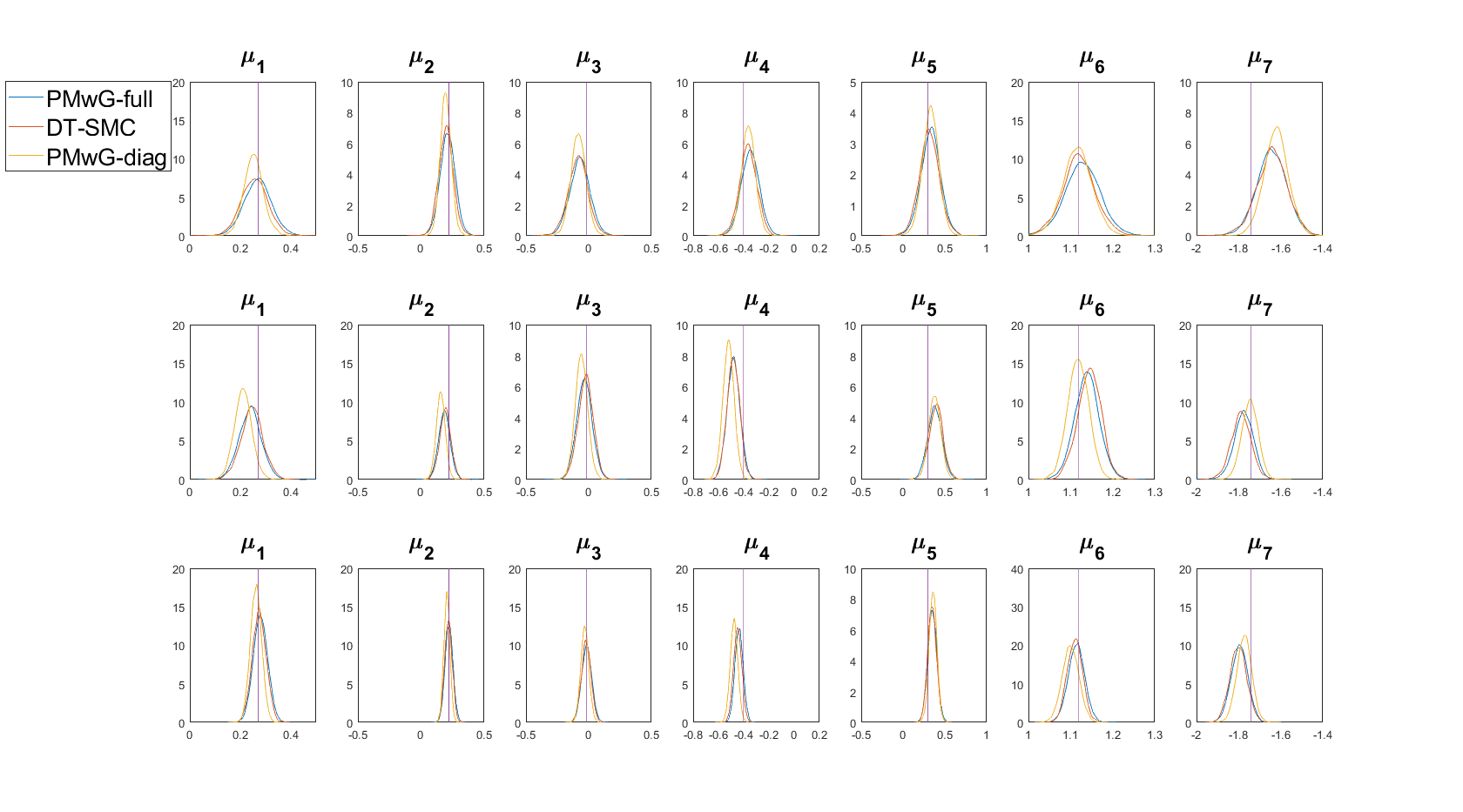
Refer to caption — Figure 1: Kernel density estimates of the LBA group level mean parameters with $S=19$ subjects (top), $S=50$ (middle), and $S=100$ (bottom) and $N=1,000$ in the simulation study. Colours represent the three sampling algorithms: PMwG (blue); density tempered SMC (red); and PMwG with a diagonal covariance matrix (no between-parameter correlations in the prior, yellow). The vertical lines show the true (data generating) values.

The two figures show that the PMwG and density tempered SMC estimators give very similar results—suggesting that the two algorithms are correctly implemented. The posterior densities narrow as the number of subjects $S$ increases, and the posterior modes of the parameters are consistent with the true data generating values. Each panel in the two figures also includes a third posterior distribution (in yellow), which illustrates the effect of making the standard hierarchical LBA assumption that the random effects are independent, using the same priors for the group level parameters as in the correlated case discussed above, and using PMwG to sample.

The results for this simplified, uncorrelated, LBA model differ systematically to the LBA model proposed here. The posterior mean estimates are more certain, that is, the distributions are more peaked (Figure 1), and the posterior variance estimates are smaller (Figure 2). This suggests that using a model with independent distributions for the random effects, as is standard in the literature, can – if there really is correlation in the data – lead to unwarranted overconfidence in estimation precision, and under-estimation of the magnitude of individual differences.

We estimated the marginal likelihood for each simulated experiment ( $S=19$ , $S=50$ , and $S=100$ subjects) using the outputs of the density tempered SMC sampler and the three estimators: the standard density tempered SMC method, and the thermodynamic integration estimators $TI_{1}$ and $TI_{2}$ discussed in Section 3.3. Table 3 reports the logs of the marginal likelihood estimates (with the standard error in brackets); the standard errors are obtained using ten replicates for each estimator. The three methods agree very closely, and the standard errors for each method are very small, suggesting that the log of the marginal likelihoods are estimated accurately.

Table 3: Logs of the marginal likelihood estimates (with standard errors in brackets).

S	N	DT-SMC	$TI_{1}$	$TI_{2}$
19	1,000	$\underset{\left(2.33\right)}{8,219.29}$	$\underset{\left(2.21\right)}{8,219.05}$	$\underset{\left(2.21\right)}{8,219.53}$
50	1,000	$\underset{\left(7.72\right)}{25,837.82}$	$\underset{\left(7.79\right)}{25,837.70}$	$\underset{\left(7.79\right)}{25,838.19}$
100	1,000	$\underset{\left(13.03\right)}{44,370.31}$	$\underset{\left(13.00\right)}{44,370.68}$	$\underset{\left(12.99\right)}{44,371.19}$

Figure 3 shows the kernel density estimates of the marginal posterior densities for the three parameters ${\boldsymbol{\mu}}_{{{1}}}$ , ${\boldsymbol{\mu}}_{{{2}}}$ and ${\boldsymbol{\mu}}_{{{3}}}$ which govern the decision threshold in the accuracy, neutral, and speed emphasis conditions (respectively) of the simulated experiment. There is considerable overlap between the two marginal distributions representing the different threshold parameters for the accuracy and neutral conditions. If these data were from a real (not simulated) experiment, this might be interpreted as evidence that the participants in the experiment failed to distinguish between those two conditions; that they did (or could) not adopt different decision-making styles when asked to.

This is exactly the kind of model selection question facing researchers using the LBA model. Section 4.2 demonstrates how to use the marginal likelihood estimates obtained using density tempered SMC to further investigate whether participants adopted different decision-making thresholds in the three conditions. In that section, we compare the unrestricted (three parameter) model against restricted models having shared threshold parameters. An alternative approach to this question could enforce order constraints on the estimated random effects. This is easily accomplished by parameter transformations – define the speed-emphasis threshold as usual, and then estimate parameters for the differences between that threshold and the neutral condition threshold, and between the neutral and accuracy condition thresholds. These incremental parameters can be constrained to be positive by estimating their logarithms, as with the other parameters, and inferential tests made by comparing the estimated increments with zero.

Comparing the PMwG sampler to existing estimation methods

The hierarchical LBA model is most often estimated using DE-MCMC as developed by Turner et al. (2013). However, such applications have been restricted to an LBA model which assumes independent truncated normal prior distributions for the random effects, whereas the LBA model defined in Section 2 allows for a (correlated) multivariate normal prior distribution on the log of the random effects. The considerably simpler model estimated via DE-MCMC does not require the estimation of covariance elements. An uncorrelated model with $D_{\alpha}$ random effects per person has $2D_{\alpha}$ group-level parameters (a mean and a standard deviation for each random effect). In contrast, the current LBA model has $D_{\alpha}+(D_{\alpha}+1)D_{\alpha}/2$ parameters (a mean and standard deviation for each random effect, plus all pairwise covariances). F shows that the PMwG sampler agrees with the DE-MCMC sampler, when estimating the simplified LBA model without correlations.

Estimating the LBA model with non-zero correlations in the prior may be impossible with the current DE-MCMC sampler and will require extensive modifications at a minimum. The DE-MCMC sampler generates the group level mean and standard deviation for each of the random effects blocked in pairs. This blocking breaks down when the off-diagonal covariances in the prior are non-zero, as they are highly correlated with the (diagonal) variance parameters, and so some other blocking scheme will need to be devised. It is not clear what that scheme should be. Further, DE-MCMC generates proposals by taking linear combinations of existing samples. When the correlations are non-zero, this means generating covariance matrix proposals, but the differential evolution approach does not ensure that the proposals will be valid covariance matrices (positive definite). It is also standard to set the tuning parameter in the DE-MCMC algorithm inversely proportional to the number of parameters. This is likely to make the method very inefficient given the much larger number of unknown parameters when a full covariance matrix is used in the prior (scales with $D_{\alpha}^{2}$ ). It is possible that these difficulties for DE-MCMC may be overcome with its further development. However, such an extension of the DE-MCMC approach is beyond the scope of this paper.

In contrast, PMwG scales well as the number of parameters increases because it uses Gibbs sampling to generate the group-level parameters. In demonstrating this scaling property, Wall et al. (2019) extend the PMwG approach to estimate a high-dimensional hierarchical LBA model with $S=110$ subjects, $N=1,350$ trials, and $D_{\alpha}=30$ individual random effects parameters—giving a covariance matrix with 435 free parameters. Gunawan et al. (2019) extend the hierarchical LBA model to allow the individual level parameters of each subject to change over blocks of the trials, thus extending the PMwG approach to estimate time-varying LBA models. Both these extensions show that the methods proposed in this article allow exploration of important psychological questions that are at present neglected due to computational intractability.

4.2 Real Data Application

We applied PMwG and density tempered SMC to the behavioural data first presented by Forstmann et al. (2008), and introduced in Section 2. PMwG and density tempered SMC were run with the same settings as in A and B, respectively. The wall-clock computation times to run PMwG and density tempered SMC were around 30 and 138 minutes, respectively, using a Matlab implementation of the algorithm and 28 CPU-cores.

Table 4 shows the estimated group-level parameters from both methods, along with the estimated posterior standard deviations and the IACT inefficiency factors for PMwG. All the IACT values are again small, indicating that the chains mixed well and that the performance of the sampler did not deteriorate markedly when moving from simulated data to real data. The posterior mean estimates and the associated posterior standard deviations from PMwG and density tempered SMC are very close to each other, providing an accuracy check on both samplers.

Table 4: Posterior means (with posterior standard deviations in brackets) and IACT of the LBA group-level parameters of the full model estimated using PMwG and density tempered SMC (DT-SMC) for the data from Forstmann et al. (2008). The order of the random effect parameters in the covariance matrix

\boldsymbol{\Sigma}

{b^{(1)}}

{b^{(2)}}

{b^{(3)}}

{A}

{v^{(1)}}

{v^{(2)}}

, and

{\tau}

Param.	Est	IACT	Est	Param.	Est	IACT	Est
	PMwG	PMwG	DT-SMC		PMwG	PMwG	DT-SMC
${\boldsymbol{\mu}}_{{{1}}}$	$\underset{\left(0.06\right)}{0.27}$	$1.22$	$\underset{\left(0.06\right)}{0.28}$	${\boldsymbol{\Sigma}}_{{11}}$	$\underset{\left(0.03\right)}{0.06}$	$1.68$	$\underset{\left(0.03\right)}{0.06}$
${\boldsymbol{\mu}}_{{{2}}}$	$\underset{\left(0.06\right)}{0.22}$	$1.17$	$\underset{\left(0.06\right)}{0.22}$	${\boldsymbol{\Sigma}}_{{22}}$	$\underset{\left(0.03\right)}{0.07}$	$1.62$	$\underset{\left(0.03\right)}{0.07}$
${\boldsymbol{\mu}}_{{{3}}}$	$\underset{\left(0.08\right)}{-0.02}$	$1.10$	$\underset{\left(0.09\right)}{-0.01}$	${\boldsymbol{\Sigma}}_{{33}}$	$\underset{\left(0.05\right)}{0.13}$	$1.49$	$\underset{\left(0.05\right)}{0.13}$
${\boldsymbol{\mu}}_{{{4}}}$	$\underset{\left(0.07\right)}{-0.40}$	$1.49$	$\underset{\left(0.07\right)}{-0.40}$	${\boldsymbol{\Sigma}}_{{44}}$	$\underset{\left(0.04\right)}{0.09}$	$2.61$	$\underset{\left(0.04\right)}{0.09}$
${\boldsymbol{\mu}}_{{{5}}}$	$\underset{\left(0.11\right)}{0.30}$	$1.26$	$\underset{\left(0.11\right)}{0.31}$	${\boldsymbol{\Sigma}}_{{55}}$	$\underset{\left(0.09\right)}{0.22}$	$2.00$	$\underset{\left(0.08\right)}{0.22}$
${\boldsymbol{\mu}}_{{{6}}}$	$\underset{\left(0.04\right)}{1.12}$	$1.28$	$\underset{\left(0.04\right)}{1.13}$	${\boldsymbol{\Sigma}}_{{66}}$	$\underset{\left(0.02\right)}{0.03}$	$2.53$	$\underset{\left(0.02\right)}{0.03}$
${\boldsymbol{\mu}}_{{{7}}}$	$\underset{\left(0.07\right)}{-1.74}$	$2.16$	$\underset{\left(0.07\right)}{-1.75}$	${\boldsymbol{\Sigma}}_{{77}}$	$\underset{\left(0.04\right)}{0.09}$	$5.70$	$\underset{\left(0.04\right)}{0.09}$
${\boldsymbol{\Sigma}}_{{12}}$	$\underset{\left(0.03\right)}{0.06}$	$1.66$	$\underset{\left(0.03\right)}{0.07}$	${\boldsymbol{\Sigma}}_{{34}}$	$\underset{\left(0.04\right)}{0.08}$	$1.53$	$\underset{\left(0.04\right)}{0.08}$
${\boldsymbol{\Sigma}}_{{13}}$	$\underset{\left(0.03\right)}{0.08}$	$1.61$	$\underset{\left(0.04\right)}{0.08}$	${\boldsymbol{\Sigma}}_{{35}}$	$\underset{\left(0.05\right)}{0.11}$	$1.59$	$\underset{\left(0.05\right)}{0.11}$
${\boldsymbol{\Sigma}}_{{14}}$	$\underset{\left(0.03\right)}{0.06}$	$1.63$	$\underset{\left(0.03\right)}{0.06}$	${\boldsymbol{\Sigma}}_{{36}}$	$\underset{\left(0.02\right)}{0.01}$	$1.56$	$\underset{\left(0.02\right)}{0.01}$
${\boldsymbol{\Sigma}}_{{15}}$	$\underset{\left(0.04\right)}{0.06}$	$1.70$	$\underset{\left(0.04\right)}{0.07}$	${\boldsymbol{\Sigma}}_{{37}}$	$\underset{\left(0.04\right)}{-0.09}$	$2.89$	$\underset{\left(0.04\right)}{-0.09}$
${\boldsymbol{\Sigma}}_{{16}}$	$\underset{\left(0.01\right)}{0.00}$	$1.61$	$\underset{\left(0.01\right)}{0.00}$	${\boldsymbol{\Sigma}}_{{45}}$	$\underset{\left(0.04\right)}{0.04}$	$1.70$	$\underset{\left(0.04\right)}{0.04}$
${\boldsymbol{\Sigma}}_{{17}}$	$\underset{\left(0.03\right)}{-0.05}$	$2.67$	$\underset{\left(0.03\right)}{-0.05}$	${\boldsymbol{\Sigma}}_{{46}}$	$\underset{\left(0.01\right)}{0.00}$	$1.60$	$\underset{\left(0.02\right)}{0.00}$
${\boldsymbol{\Sigma}}_{{23}}$	$\underset{\left(0.04\right)}{0.09}$	$1.56$	$\underset{\left(0.04\right)}{0.09}$	${\boldsymbol{\Sigma}}_{{47}}$	$\underset{\left(0.03\right)}{-0.05}$	$2.00$	$\underset{\left(0.03\right)}{-0.05}$
${\boldsymbol{\Sigma}}_{{24}}$	$\underset{\left(0.03\right)}{0.06}$	$1.56$	$\underset{\left(0.03\right)}{0.06}$	${\boldsymbol{\Sigma}}_{{56}}$	$\underset{\left(0.02\right)}{0.01}$	$1.58$	$\underset{\left(0.02\right)}{0.01}$
${\boldsymbol{\Sigma}}_{{25}}$	$\underset{\left(0.04\right)}{0.08}$	$1.72$	$\underset{\left(0.04\right)}{0.08}$	${\boldsymbol{\Sigma}}_{{57}}$	$\underset{\left(0.05\right)}{-0.09}$	$2.82$	$\underset{\left(0.05\right)}{-0.10}$
${\boldsymbol{\Sigma}}_{{26}}$	$\underset{\left(0.01\right)}{0.01}$	$1.71$	$\underset{\left(0.01\right)}{0.01}$	${\boldsymbol{\Sigma}}_{{67}}$	$\underset{\left(0.01\right)}{0.00}$	$1.57$	$\underset{\left(0.01\right)}{0.00}$
${\boldsymbol{\Sigma}}_{{27}}$	$\underset{\left(0.03\right)}{-0.06}$	$3.05$	$\underset{\left(0.03\right)}{-0.06}$

Figure 4 shows the kernel density estimates of marginal posterior densities for the group mean parameters, using samples from PMwG (blue) and density tempered SMC (red); the figure also shows the estimated posterior distributions for the reduced model, with zero prior correlation between the individual level parameters estimated using PMwG (yellow). Figure 5 shows the corresponding results for the between-subject variance parameters instead of the means, i.e., the diagonal elements of $\Sigma$ . Both figures demonstrate that the density tempered SMC estimates are very close to the PMwG estimates, for all the parameters for the LBA model with a full prior covariance matrix for the random effects. However, similarly to the simulation study, the posterior estimates from the simplified LBA model (with zero covariance) are quite different to the posterior estimates from the LBA model with a full covariance matrix. The differences are particularly pronounced for the variance parameters in Figure 5. In all cases, the zero-covariance reduced model estimates are much smaller for the between-subjects variances, and often also have narrower posterior distributions. This matches the results from the simulation study above, and is consistent with the hypothesis that the real data includes non-zero between-subject correlations, and failing to take this into account in the prior leads to unwarranted overconfidence in the posteriors.

The model setup in Section 2 allows us to estimate the correlation matrix $\Gamma$ between individual level parameters by using the standard transformation of the estimated covariance matrix. Table 5 shows that the threshold parameters for all three conditions are highly correlated: $\Gamma\left(b^{(1)},b^{(2)}\right)=.96$ , $\Gamma\left(b^{(1)},b^{(3)}\right)=.87$ , and $\Gamma\left(b^{(2)},b^{(3)}\right)=.93$ . The maximum value of the start point distribution ( $A$ ) is also highly correlated with the threshold parameters; $\Gamma\left(b^{(1)},A\right)=.80$ , $\Gamma\left(b^{(2)},A\right)=.76$ , and $\Gamma\left(b^{(3)},A\right)=.70$ . The non-decision time parameters at the individual subject level are negatively correlated with all other individual level parameters – presumably because of trade-offs between explaining the same RT as either composed of more or less decision time vs. non-decision time. The mean drift rate for the accumulator corresponding to the correct response is not highly correlated with other individual level parameters. The magnitudes of these correlations emphasize the importance of explicitly modelling the covariance matrix, rather than forcing it to have zero correlations.

Table 5: Posterior means (with posterior standard deviations in brackets) of the correlations of the LBA parameters obtained using density tempered SMC.

Param	Est.	Param	Est.	Param	Est.
$\Gamma{\left(b^{\left(1\right)},b^{\left(2\right)}\right)}$	$\underset{\left(0.02\right)}{0.96}$	$\Gamma{\left(b^{\left(2\right)},A\right)}$	$\underset{\left(0.12\right)}{0.76}$	$\Gamma{\left(b^{\left(3\right)},\tau\right)}$	$\underset{\left(0.06\right)}{-0.70}$
$\Gamma{\left(b^{\left(1\right)},b^{\left(3\right)}\right)}$	$\underset{\left(0.05\right)}{0.87}$	$\Gamma{\left(b^{\left(2\right)},v^{\left(1\right)}\right)}$	$\underset{\left(0.14\right)}{0.57}$	$\Gamma{\left(A,v^{\left(1\right)}\right)}$	$\underset{\left(0.20\right)}{0.27}$
$\Gamma{\left(b^{\left(1\right)},A\right)}$	$\underset{\left(0.10\right)}{0.80}$	$\Gamma{\left(b^{\left(2\right)},v^{\left(2\right)}\right)}$	$\underset{\left(0.23\right)}{0.09}$	$\Gamma{\left(A,v^{\left(2\right)}\right)}$	$\underset{\left(0.23\right)}{-0.03}$
$\Gamma{\left(b^{\left(1\right)},v^{\left(1\right)}\right)}$	$\underset{\left(0.16\right)}{0.49}$	$\Gamma{\left(b^{\left(2\right)},\tau\right)}$	$\underset{\left(0.07\right)}{-0.69}$	$\Gamma{\left(A,\tau\right)}$	$\underset{\left(0.16\right)}{-0.46}$
$\Gamma{\left(b^{\left(1\right)},v^{\left(2\right)}\right)}$	$\underset{\left(0.23\right)}{0.03}$	$\Gamma{\left(b^{\left(3\right)},A\right)}$	$\underset{\left(0.14\right)}{0.70}$	$\Gamma{\left(v^{\left(1\right)},v^{\left(2\right)}\right)}$	$\underset{\left(0.22\right)}{0.16}$
$\Gamma{\left(b^{\left(1\right)},\tau\right)}$	$\underset{\left(0.09\right)}{-0.63}$	$\Gamma{\left(b^{\left(3\right)},v^{\left(1\right)}\right)}$	$\underset{\left(0.14\right)}{0.62}$	$\Gamma{\left(v^{\left(1\right)},\tau\right)}$	$\underset{\left(0.09\right)}{-0.55}$
$\Gamma{\left(b^{\left(2\right)},b^{\left(3\right)}\right)}$	$\underset{\left(0.03\right)}{0.93}$	$\Gamma{\left(b^{\left(3\right)},v^{\left(2\right)}\right)}$	$\underset{\left(0.23\right)}{0.14}$	$\Gamma{\left(v^{\left(2\right)},\tau\right)}$	$\underset{\left(0.22\right)}{-0.03}$

Table 6 summarizes the posterior mean estimates of the parameters on the original (not logarithmic) scale obtained using Eq. (6). These values suggest that there may only be slight differences in the estimates of the threshold parameters between the three conditions: accuracy, neutral, and speed ( $\tilde{{\mu}}_{1}$ , $\tilde{{\mu}}_{2}$ , and $\tilde{{\mu}}_{3}$ ). To investigate this, we estimated a restricted model with two threshold parameters by combining the accuracy and neutral conditions, as well as a more restricted model with a single, shared, threshold parameter for all three conditions. We used density tempered SMC, specified as above, to estimate the marginal likelihood for each model. Table 7 reports the estimated log marginal likelihoods (with standard errors in brackets) for the three models. The differences between the log marginal likelihoods are much larger than the standard errors, and also large relative to the scales usually used to judge statistical reliability, e.g. the corresponding Bayes factors for the model comparisons are all much larger than $10^{6}$ . The results favour the unrestricted model for these data, which also supports the analyses by Forstmann et al. (2008). An important caveat for this analysis is that the marginal likelihoods – for any model – depend on the prior. For example, another approach to the problem would set up the random effects using an intercept plus effect coding, and specify a prior distribution for the effect sizes. Further work will be required to investigate the sensitivity of model selection outcomes to different choices of prior distribution.

Table 6: Posterior means (with posterior standard deviations in brackets) of the group level LBA parameters of the model with three threshold parameters on the original (not logarithmic) scale obtained using Eq. (6). The order of the random effect parameters is the same as defined in Section 2.

Param.	Est.	Param	Est.
$\tilde{{\mu}}_{1}$	$\underset{\left(0.08\right)}{1.36}$	$\tilde{\Sigma}_{1,1}$	$\underset{\left(0.06\right)}{0.13}$
$\tilde{{\mu}}_{2}$	$\underset{\left(0.09\right)}{1.30}$	$\tilde{\Sigma}_{2,2}$	$\underset{\left(0.06\right)}{0.13}$
$\tilde{{\mu}}_{3}$	$\underset{\left(0.09\right)}{1.06}$	$\tilde{\Sigma}_{3,3}$	$\underset{\left(0.09\right)}{0.16}$
$\tilde{{\mu}}_{4}$	$\underset{\left(0.05\right)}{0.70}$	$\tilde{\Sigma}_{4,4}$	$\underset{\left(0.03\right)}{0.05}$
$\tilde{{\mu}}_{5}$	$\underset{\left(0.18\right)}{1.52}$	$\tilde{\Sigma}_{5,5}$	$\underset{\left(0.37\right)}{0.60}$
$\tilde{{\mu}}_{6}$	$\underset{\left(0.14\right)}{3.14}$	$\tilde{\Sigma}_{6,6}$	$\underset{\left(0.17\right)}{0.34}$
$\tilde{{\mu}}_{7}$	$\underset{\left(0.01\right)}{0.18}$	$\tilde{\Sigma}_{7,7}$	$\underset{\left(0.002\right)}{0.003}$

Table 7: Log of the marginal likelihood estimates (with standard errors in brackets), for the three models with different numbers of free threshold parameters (1, 2, or 3).

Thresholds	Standard density tempered SMC	$TI_{1}$	$TI_{2}$
One	$\underset{\left(1.59\right)}{5,200.58}$	$\underset{\left(1.52\right)}{5,200.48}$	$\underset{\left(1.52\right)}{5,200.99}$
Two	$\underset{\left(2.38\right)}{7,350.80}$	$\underset{\left(2.24\right)}{7,350.56}$	$\underset{\left(2.23\right)}{7,351.05}$
Three	$\underset{\left(3.10\right)}{7,447.31}$	$\underset{\left(3.04\right)}{7,447.28}$	$\underset{\left(3.04\right)}{7,447.75}$

5 Conclusions

Based on recent advances in particle MCMC, the article develops two new estimation approaches for the Linear Ballistic Accumulator model of Brown and Heathcote (2008); Particle Metropolis within Gibbs and density tempered SMC. We show that PMwG and density tempered SMC perform well for both simulated and real data. The new methods are alternatives to the existing approach that is based on MCMC with proposals generated by differential evolution (Turner et al., 2013) and provide important advantages. Density tempered SMC is extremely well-suited to parallelisation on high-performance computers, which is likely to be an advantage in future work with large-scale models and data. Although both PMwG and DE-MCMC are also both appropriate for parallelisation in high-performance computing environments, DE-MCMC requires more frequent dependence between the multiple chains, which limits its efficiency when parallelised. We also found that the PMwG sampler is much faster than density tempered SMC and can be easily implemented with minimal computational resources, e.g., personal computers. Furthermore, density tempered SMC provides an estimate of the marginal likelihood at little extra cost, and hence it can be readily used for model selection via Bayes factors.

Another important contribution of our work is to explicitly model the full covariance structure of the prior for the random effects. Like all plausible cognitive models, there are substantial correlations between the individual level parameters of the LBA model: subjects with a large decision threshold also tend to have a large starting point distribution, etc. In previous applications of the model, these prior correlations were set to zero, with the group-level distributions treated a priori as independent. Despite making this a priori assumption of independence, the resulting posterior samples always exhibited strong posterior correlations between individual level parameters. Explicitly allowing non-zero correlations in the prior, as we have done, provides better estimates of the parameters and their variances, and improves computational efficiency.

The computational flexibility of the new methods allows exploration of important psychological questions which have hitherto been neglected, due to statistical intractability. For example, it is well known that there can be substantial sequential effects in decision-making data: both response choices and response times tend to be positively autocorrelated. All applications of the LBA model – and indeed, almost all decision-making models – have ignored these sequential effects, treating the data as i.i.d. and attributing the effects of any sequential dependence to error terms. Both our approaches allow tractable extensions that explicitly take into account of within subject dependence and other interesting sequential effects such as parameter evolution due to fatigue or learning. We are investigating these models in ongoing work.

To aid researchers in adopting the proposed methods, we provide scripts that implement both the PMwG and density tempered SMC methods as applied to the real data from Forstmann et al. (2008); see osf.io/5b4w3 for more details.

Acknowledgements

We thank three anonymous referees and an Action editor for comments that improved the scientific content and clarity of the paper. The research of Gunawan, Tran, Kohn and Brown was partially supported by the Australian Research Council (ARC) Discovery grant DP180102195; Gunawan and Kohn were also supported by ARC Discovery grant DP150104630; and Hawkins by the ARC DECRA grant DE170100177.

6 References

References

Annis et al. (2017) Annis, J., Miller, B. J., Palmeri, T. J., 2017. Bayesian inference with Stan: a tutorial on adding custom distributions. Behavioural Research 49 (863-886).
Atkinson and Han (2004) Atkinson, K., Han, W., 2004. Elementary Numerical Analysis, 3rd edn. New York, John Wiley.
Betancourt (2018) Betancourt, M., 2018. A conceptual introduction to Hamiltonian Monte Carlo. arXiv:1701.02434v2.
Brown and Heathcote (2005) Brown, S., Heathcote, A., 2005. A ballistic model of choice response time. Psychological Review 112, 117–128.
Brown and Heathcote (2008) Brown, S., Heathcote, A., 2008. The simple complete model of choice reaction time: Linear Ballistic accumulation. Cognitive Psychology 57, 153–178.
Chib and Greenberg (1996) Chib, S., Greenberg, E., 1996. Markov chain Monte Carlo simulation methods in econometrics. Econometrics Theory (12), 409–431.
Chib and Jeliazkov (2001) Chib, S., Jeliazkov, I., 2001. Marginal likelihood from the Metropolis-Hastings output. Journal of American Statistical Association 96 (453), 270–281.
Del Moral et al. (2006) Del Moral, P., Doucet, A., Jasra, A., 2006. Sequential Monte Carlo samplers. Journal of the Royal Statistical Society, Series B 68, 411–436.
Del Moral et al. (2012) Del Moral, P., Doucet, A., Jasra, A., 2012. An adaptive Sequential Monte Carlo for approximate Bayesian computation. Statistics and Computing, 1009–1020.
Donkin and Brown (2018) Donkin, C., Brown, S. D., 2018. Response times and decision-making. Stevens’ Handbook of Experimental Psychology and Cognitive Neuroscience, Methodology, 349.
Donkin et al. (2009) Donkin, C., Brown, S. D., Heathcote, A. J., 2009. The over-constraint of response time models: Rethinking the scaling problem. Psychonomic Bulletin & Review 16, 1129–1135.
Duan and Fulop (2015) Duan, J. C., Fulop, A., 2015. Density-tempered marginalised sequential Monte Carlo samplers. Journal of Business and Economics Statistics 33 (2), 192–202.
Evans and Annis (2019) Evans, N. J., Annis, J., 2019. Thermodynamic integration via differential evolution: a method for estimating marginal likelihood. Behavior Research Methods 51, 930–947.
Evans and Brown (2018) Evans, N. J., Brown, S. D., 2018. Bayes factors for the linear ballistic accumulator model of decision-making. Behavior research methods 50 (2), 589–603.
Evans et al. (2018) Evans, N. J., Steyvers, M., Brown, S. D., 2018. Modeling the covariance structure of complex datasets using cognitive models: An application to individual differences and the heritability of cognitive ability. Cognitive science 42 (6), 1925–1944.
Forstmann et al. (2008) Forstmann, B. U., Dutilh, G., Brown, S., Neumann, J., von Cramon, D. Y., 2008. Striatum and pre-sma facilitate decision making under time pressure. Proceedings of the National Academy of Sciences 105, 17538–17542.
Friel et al. (2014) Friel, N., Hurn, M., Wyse, J., 2014. Improving power posterior estimation of statistical evidence. Statistics and Computing 24 (5), 709–723.
Friel and Pettitt (2008) Friel, N., Pettitt, A. N., 2008. Marginal likelihood estimation via power posteriors. Journal of the Royal Statistical Society: Series B (Statistical Methodology) 70 (3), 589–607.
Gelman and Meng (1998) Gelman, A., Meng, X.-L., 1998. Simulating normalizing constants: From importance sampling to bridge sampling to path sampling. Statistical Science, 163–185.
Gronau et al. (2019) Gronau, Q. F., Heathcote, A., Matzke, D., 2019. Computing bayes factors for evidence accumulation models using warp-iii bridge sampling. Behavior Research Methods, https://doi.org/10.3758/s13428-019-01290-6.
Gunawan et al. (2017) Gunawan, D., Carter, C., Fiebig, D. G., Kohn, R., 2017. Efficient Bayesian estimation for flexible panel models for multivariate outcomes: impact of life events on mental health and excessive alcohol consumption. arXiv preprint arXiv:1706.03953v1.
Gunawan et al. (2019) Gunawan, D., E.Hawkins, G., Kohn, R., Tran, M. N., Brown, S. D., 2019. Time-evolving psychological processes over repeated decisions. arXiv:1906.10838v1.
Hesterberg (1995) Hesterberg, T., 1995. Weighted average importance sampling and defensive mixture distributions. Technometrics 37, 185–194.
Huang and Wand (2013) Huang, A., Wand, M. P., 2013. Simple marginally noninformative prior distributions for covariance matrices. Bayesian Analysis 8 (2), 439–452.
Kass and Raftery (1995) Kass, R. E., Raftery, A. E., 1995. Bayes factors. Journal of American Statistical Association 90 (430), 773–795.
Neal (2001) Neal, R., 2001. Annealed importance sampling. Statistics and Computing 11, 125–139.
Plummer et al. (2006) Plummer, M., Best, N., Cowles, K., Vines, K., 2006. CODA: Convergence Diagnosis and Output Analysis of MCMC. R News 6 (1), 7–11.
Ratcliff (1978) Ratcliff, R., 1978. A theory of memory retrieval. Psychological Review 85, 59–108.
Ratcliff and Rouder (1998) Ratcliff, R., Rouder, J. N., 1998. Modeling response times for two–choice decisions. Psychological Science 9, 347–356.
Ratcliff and Smith (2004) Ratcliff, R., Smith, P. L., 2004. A comparison of sequential sampling models for two–choice reaction time. Psychological Review 111, 333–367.
Ratcliff et al. (2016) Ratcliff, R., Smith, P. L., Brown, S. D., McKoon, G., 2016. Diffusion decision model: current issues and history. Trends in cognitive sciences 20 (4), 260–281.
Spiegelhalter et al. (2014) Spiegelhalter, D. J., Best, N. G., Carlin, B. P., Linde, A., 2014. The deviance information criterion: 12 years on. Journal of the Royal Statistical Society: Series B (Statistical Methodology) 76 (3), 485–493.
Terry et al. (2015) Terry, A., Marley, A., Barnwal, A., Wagenmakers, E.-J., Heathcote, A., Brown, S. D., 2015. Generalising the drift rate distribution for linear ballistic accumulators. Journal of Mathematical Psychology 68, 49–58.
Turner et al. (2013) Turner, B. M., Sederberg, P. B., Brown, S. D., Steyvers, M., 2013. A method for efficiently sampling from distributions with correlated dimensions. Psychological Methods 18 (3), 368–384.
Usher and McClelland (2001) Usher, M., McClelland, J. L., 2001. On the time course of perceptual choice: The leaky competing accumulator model. Psychological Review 108, 550–592.
Wall et al. (2019) Wall, L., Gunawan, D., Brown, S. D., Tran, M. N., Kohn, R., Hawkins, G. E., 2019. Identifying relationships between cognitive processes across tasks, contexts, and time. arXiv:1910.07185v1.
Watanabe (2010) Watanabe, S., 2010. Asymptotic equivalence of bayes cross validation and widely applicable information criterion in singular learning theory. Journal of Machine Learning Research 11 (Dec), 3571–3594.
Xie et al. (2010) Xie, W., Lewis, P. O., Fan, Y., Kuo, L., Chen, M. H., 2010. Improving marginal likelihood estimation for Bayesian phylogenetic model selection. Systematic Biology 60 (2), 150–160.

Appendix A Tuning parameters and proposal densities for the PMwG sampler

For PMwG, it is necessary to specify the number of particles $R$ , and the proposal densities $m_{j}\left(\boldsymbol{\alpha}_{j}|\boldsymbol{\theta},\boldsymbol{y}_{j}\right)$ , for each subject $j=1,...,S$ . Gunawan et al. (2017) use the prior densities $p\left(\boldsymbol{\alpha}_{j}|\boldsymbol{\mu},\boldsymbol{\Sigma}\right)$ as the proposal densities for the random effects. The practical performance of the algorithm is greatly enhanced by choosing efficient proposal densities. To simplify this choice, we develop efficient proposal densities in three stages: burnin, initial adaptation, and sampling. In the burnin and the initial adaptation stages, the proposal density for subject $j$ is a mixture over the prior group-level distribution for the random effects, $p\left(\boldsymbol{\alpha}_{j}|\boldsymbol{\theta}\right)$ , and a normal distribution centred on the previous sample for the random effect $N\big(\boldsymbol{\alpha}_{j};\boldsymbol{\alpha}_{j}^{\left(iter-1\right)},\boldsymbol{\Sigma}\big)$ ,

m_{j}\left(\boldsymbol{\alpha}_{j}|\boldsymbol{\theta},\boldsymbol{y}_{j}\right)=w_{mix}N\big(\boldsymbol{\alpha}_{j};\boldsymbol{\alpha}_{j}^{\left(iter-1\right)},\boldsymbol{\Sigma}\big)+\left(1-w_{mix}\right)p\left(\boldsymbol{\alpha}_{j}|\boldsymbol{\theta}\right),

(18)

where $\boldsymbol{\alpha}_{j}^{\left(iter-1\right)}$ is the previous iterate $\boldsymbol{\alpha}_{j}^{k_{j}}$ for the individual $j$ th random effect. In practice, we should use a larger number of particles in the burnin and initial adaptation stages than in the sampling stages.

This proposal can be made more flexible by using $\epsilon\boldsymbol{\Sigma}$ instead of $\boldsymbol{\Sigma}$ , where $0<\epsilon<1$ is a scale factor. In this paper, we set $\epsilon=1$ . It is necessary to reduce the scale factor $\epsilon$ when we have larger number of random effects. Wall et al. (2019) estimate a high-dimensional hierarchical LBA model with $S=110$ subjects, $N=1,350$ trials, and $D_{\alpha}=30$ individual random effects parameters and set $\epsilon=0.1$ . We find empirically in our examples that this strategy works well in practice.

In the sampling stage, we use the posterior MCMC draws $\left(\boldsymbol{\alpha}_{1:S},\boldsymbol{\theta}\right)$ from the initial adaptation stage to adaptively build more efficient proposal densities $m_{j}\left(\boldsymbol{\alpha}_{j}|\boldsymbol{\theta},\boldsymbol{y}_{j}\right)$ , for each subject $j=1,...,S$ . This usually allows the use of a much smaller number of particles. We first transform the posterior draws of the parameters $\boldsymbol{\Sigma}$ so that they all lie on the real line. The covariance matrix $\boldsymbol{\Sigma}$ is reparameterised in terms of its Cholesky factorisation $\boldsymbol{\Sigma}=\boldsymbol{L}\boldsymbol{L}^{T}$ , where $\boldsymbol{L}$ is a lower triangular matrix. We also apply a log transformation for the diagonal elements of $\boldsymbol{L}$ , while the subdiagonal elements of $\boldsymbol{L}$ are unrestricted. For each subject, we fit a normal distribution to the vectors formed by joining the posterior draws of $\boldsymbol{\alpha}_{j}$ with $\left(\boldsymbol{\mu},\boldsymbol{L}\right)$ and obtain the conditional distribution $g\left(\boldsymbol{\alpha}_{j}|\boldsymbol{\mu},\boldsymbol{L}\right)\sim N\left(\boldsymbol{\alpha}_{j};\boldsymbol{\mu}_{j,prop},\boldsymbol{\Sigma}_{j,prop}\right)$ for $j=1,...,S$ . The efficient proposal density for subject $j$ is then the two component mixture

m_{j}\left(\boldsymbol{\alpha}_{j}|\boldsymbol{\theta},\boldsymbol{y}_{j}\right)=w_{mix}N\left(\boldsymbol{\alpha}_{j};\boldsymbol{\mu}_{j,prop},\boldsymbol{\Sigma}_{j,prop}\right)+\left(1-w_{mix}\right)p\left(\boldsymbol{\alpha}_{j}|\boldsymbol{\theta}\right).

(19)

In this paper, the number of particles in the PMwG method is set to $R_{burnin}=R_{adapt}=R_{sampling}=100$ ; as discussed above, it is sometimes helpful to use more particles in the burnin and initial adaptation stages. We also set $w_{mix}=0.9$ .

We used $500$ burnin iterations, $500$ adaptation iterations, and $10000$ iterations for sampling. Following Hesterberg (1995), including the prior density $p\left(\boldsymbol{\alpha}_{j}|\boldsymbol{\theta}\right)$ in Eq. (18) and Eq. (19) ensures that the importance weights are bounded because it is straightforward to show that the density $p\left(\boldsymbol{y}_{j}|\boldsymbol{\theta},\boldsymbol{\alpha}_{j}\right)$ is bounded. This ensures that the sampler is ergodic; see the online supplement at osf.io/5b4w3 for further details.

Appendix B Tuning Parameters and Proposal Densities for Density tempered SMC

Density tempered SMC has three tuning parameters: the number of particles $R$ , the number of Markov move steps $L$ , and the number of SMC samples $M$ . The bigger the number of SMC samples $M$ , the better the approximation to the posterior density $p\left(\boldsymbol{\theta},\boldsymbol{\alpha}|\boldsymbol{y}\right)$ . By using the result of Del Moral et al. (2006), density tempered SMC provides consistent inference for the posterior density $p\left(\boldsymbol{\theta},\boldsymbol{\alpha}|\boldsymbol{y}\right)$ as the number of annealed samples $M$ goes to infinity, for any given number of particles $R$ . The $L$ Markov moves in step (2e) in Algorithm 3 help to diversify the collection of parameters and random effects after the resampling in step (2d) so that they better approximate the tempered target density. In addition, we can obtain more accurate marginal likelihood estimates with larger number of SMC samples $M$ , the number of particles $R$ , and the number of Markov move steps $L$ .

The prior density $p\left(\boldsymbol{\alpha}_{j}|\boldsymbol{\theta}\right)$ is an efficient proposal for the random effects for each subject when the tempering value $a_{p}$ is small as it dominates the tempered density which is quite flat because $p\left(\boldsymbol{y}_{j}|\boldsymbol{\theta},\boldsymbol{\alpha}_{j}\right)^{a_{p}}\approx 1$ . In our application we use the prior as a proposal density when $a_{p}<0.1$ . It is often also adequate to use a smaller number of particles $R$ and smaller number of Markov moves $L$ when $a_{p}$ is small. When $a_{p}$ is larger than 0.1, we first fit a normal distribution – in the same manner as for the adaptive proposal densities in the PMwG algorithm – to the current transformed particle cloud $\big\{\left(\boldsymbol{\mu},\boldsymbol{L}\right)_{1:M}^{\left(p\right)},\boldsymbol{\alpha}_{j,1:M}^{\left(p\right)},W_{1:M}^{\left(p\right)}\big\}$ for $j=1,...,S$ . This gives the conditional distribution $g\left(\boldsymbol{\alpha}_{j}|\boldsymbol{\mu},\boldsymbol{L}\right)\sim N\left(\boldsymbol{\alpha}_{j};\boldsymbol{\mu}_{j,prop},\boldsymbol{\Sigma}_{j,prop}\right)$ at each stage of the SMC process. We then use the two component mixture given in Eq. (19) as a proposal density and set the mixture weight to $w_{mix}=0.9$ . The number of MC samples and Markov moves were set to $R=100$ and $L=10$ respectively. We set $ESS_{T}=0.8M$ ; i.e., we target an effective sample size of 80% of the maximum SMC sample size. Unlike the PMwG algorithm, density tempered SMC does not require an initial adaptation stage to construct the efficient proposal density. Instead, the proposal densities of the random effects for each subject are obtained from the current particle cloud at each stage of the SMC process.

Appendix C Details on the Thermodynamic Integration

The first order quadrature approximation $\left(TI_{1}\right)$ to the integral in Eq. (17) of the main text is based on the trapezoidal rule and is

\widehat{\log p\left(y\right)}=\sum_{p=1}^{P}\left(\frac{a_{p}-a_{p-1}}{2}\right)\\ \left({\mathbb{E}}_{\xi_{a_{p}}}\left(\log\left\{p\left(\boldsymbol{y}|\boldsymbol{\theta},\boldsymbol{\alpha}\right)\right\}\right)+{\mathbb{E}}_{\xi_{a_{p-1}}}\left(\log\left\{p\left(\boldsymbol{y}|\boldsymbol{\theta},\boldsymbol{\alpha}\right)\right\}\right)\right).

(20)

Discretising the tempering sequence $a_{p}$ and using the trapezoidal rule introduces some bias to the estimate in Eq. (20). Friel et al. (2014) propose using the corrected trapezium rule method of Atkinson and Han (2004) to reduce the bias of $TI_{1}$ . The corrected trapezium rule approximates the integral of a function $f$ between points $a$ and $b$ as

\int_{a}^{b}f\left(x\right)dx\approx\left(b-a\right)\left[\frac{f\left(a\right)+f\left(b\right)}{2}\right]-\frac{\left(b-a\right)^{3}}{12}f^{{}^{\prime\prime}}\left(c\right),

(21)

where $c\in\left[a,b\right]$ and $f^{{}^{\prime}}\left(\cdot\right)$ and $f^{{}^{\prime\prime}}\left(\cdot\right)$ are the first and second derivative of $f$ . The first term in Eq. (21) is the usual trapezium rule approximation used in $TI_{1}$ . The second derivative $f^{{}^{\prime\prime}}\left(c\right)$ in the second term of Eq. (21) can be approximated as

f^{{}^{\prime\prime}}\left(c\right)\approx\frac{f^{{}^{\prime}}\left(b\right)-f^{{}^{\prime}}\left(a\right)}{b-a}.

Hence,

\int_{a}^{b}f\left(x\right)dx\approx\left(b-a\right)\left[\frac{f\left(a\right)+f\left(b\right)}{2}\right]-\frac{\left(b-a\right)^{2}}{12}\left(f^{{}^{\prime}}\left(b\right)-f^{{}^{\prime}}\left(a\right)\right).

(22)

Differentiating $E_{\xi_{a_{p}}}\left(\log\left\{p\left(\boldsymbol{y}|\boldsymbol{\theta},\boldsymbol{\alpha}\right)\right\}\right)$ with respect to $a_{p}$ yields

	$\displaystyle\frac{d}{dt}E_{\xi_{a_{p}}}\left(\log\left\{p\left(\boldsymbol{y}\|\boldsymbol{\theta},\boldsymbol{\alpha}\right)\right\}\right)$	$\displaystyle=$	$\displaystyle{\mathbb{E}}_{\xi_{a_{p}}}\left(\log\left\{p\left(\boldsymbol{y}\|\boldsymbol{\theta},\boldsymbol{\alpha}\right)\right\}^{2}\right)-\left({\mathbb{E}}_{\xi_{a_{p}}}\left(\log\left\{p\left(\boldsymbol{y}\|\boldsymbol{\theta},\boldsymbol{\alpha}\right)\right\}\right)\right)^{2}$		(23)
		$\displaystyle=$	$\displaystyle{\mathbb{V}}_{\xi_{a_{p}}}\left(\log\left\{p\left(\boldsymbol{y}\|\boldsymbol{\theta},\boldsymbol{\alpha}\right)\right\}\right).$		(23)

Using the results in Eq. (23), the second order quadrature approximation $\left(TI_{2}\right)$ to the integral in Eq. (17) of the main text is

\widehat{\log p\left(y\right)}=\sum_{p=1}^{P}\left(\frac{a_{p}-a_{p-1}}{2}\right)\\ \times\left[{\mathbb{E}}_{\xi_{a_{p}}}\left(\log\left\{p\left(\boldsymbol{y}|\boldsymbol{\theta},\boldsymbol{\alpha}\right)\right\}\right)+{\mathbb{E}}_{\xi_{a_{p-1}}}\left(\log\left\{p\left(\boldsymbol{y}|\boldsymbol{\theta},\boldsymbol{\alpha}\right)\right\}\right)\right]\\ -\sum_{p=1}^{P}\frac{\left(a_{p}-a_{p-1}\right)^{2}}{12}\\ \left[{\mathbb{V}}_{\xi_{a_{p}}}\left(\log\left\{p\left(\boldsymbol{y}|\boldsymbol{\theta},\boldsymbol{\alpha}\right)\right\}\right)-{\mathbb{V}}_{\xi_{a_{p-1}}}\left(\log\left\{p\left(\boldsymbol{y}|\boldsymbol{\theta},\boldsymbol{\alpha}\right)\right\}\right)\right],

(24)

where both the expectation ${\mathbb{E}}_{\xi_{a_{p}}}\left(\log\left\{p\left(\boldsymbol{y}|\boldsymbol{\theta},\boldsymbol{\alpha}\right)\right\}\right)$ and variance
${\mathbb{V}}_{\xi_{a_{p}}}\left(\log\left\{p\left(\boldsymbol{y}|\boldsymbol{\theta},\boldsymbol{\alpha}\right)\right\}\right)$ can be estimated using the density tempered SMC output at the tempering value $a_{p}$ . See C for more details.

Estimating the marginal likelihood using thermodynamic integration requires careful consideration of three tuning issues: (i) the algorithm that samples from the tempered posterior $\xi_{a_{p}}\left(\boldsymbol{\theta},\boldsymbol{\alpha}|\boldsymbol{y}\right)$ , for $p=0,...,P$ ; (ii) the number of tempering steps $\left(P\right)$ ; and (iii) the tempering sequence $a_{p}$ for $p=0,...,P$ . Friel and Pettitt (2008) use standard MCMC algorithms, such as Gibbs and Metropolis-Hastings, because they deal with tractable likelihoods; Evans and Annis (2019) use DE-MCMC to sample from the tempered target posterior. It is important to make sure that the MCMC sampler used converges for each value of the tempering sequence $a_{p}$ , $p=0,...,P$ to ensure the accuracy of the marginal likelihood estimates. However, it is difficult in general to assess whether the chains mix adequately and converge to the invariant tempered target density. Furthermore, standard random walk Metropolis-Hastings and DE-MCMC algorithms usually suffer from high autocorrelations between samples, and slow or uncertain convergence for models with a large number of parameters. The MCMC convergence problems can sometimes be solved by increasing the number of MCMC samples, but this leads to increased computational workload and the MCMC algorithms suffer from limited parallelizability. Friel and Pettitt (2008), Xie et al. (2010), and Evans and Annis (2019) use the tempering sequence $a_{p}=\left((p-1)/(P-1)\right)^{1/0.3}$ , for $p=0,...,P$ . These tempering sequences place more computational effort on temperatures near $0$ , where the tempered posterior changes rapidly. They also fix the tempering steps before running the algorithm by experimenting with different numbers of tempering steps and then choose the tempering step $P$ that gives the lowest standard error of the log of marginal likelihood estimates. In contrast, our approach through density tempered SMC gives a principled, but perhaps not optimal, sequence of tempering steps.

Appendix D Assumptions for the Proposal Densities

We define the support of the posterior and the proposal densities as

\displaystyle\mathcal{S}_{j}^{\boldsymbol{\theta}}\coloneqq\left(\boldsymbol{\alpha}_{j}\in\boldsymbol{\chi}_{\alpha}:p\left(\boldsymbol{\alpha}_{j}|\boldsymbol{\theta},\boldsymbol{y}_{j}\right)>0\right)

and

\displaystyle\mathcal{Q}_{j}^{\boldsymbol{\theta}}\coloneqq\left\{\boldsymbol{\alpha}_{j}\in\boldsymbol{\chi}_{\alpha}:m_{j}\left(\boldsymbol{\alpha}_{j}|\boldsymbol{\theta},\boldsymbol{y}_{j}\right)>0\right\}.

and assume that $\mathcal{S}_{j}^{\boldsymbol{\theta}}\subseteq\mathcal{Q}_{j}^{\boldsymbol{\theta}}$ for any $\boldsymbol{\theta}\in R^{d_{\theta}}$ and $j=1,...,S$ . This ensures that the $m_{j}\left(\boldsymbol{\alpha}_{j}|\boldsymbol{\theta},\boldsymbol{y}_{j}\right)$ can be used as proposal densities to approximate $p\left(\boldsymbol{\alpha}_{j}|\boldsymbol{\theta},\boldsymbol{y}_{j}\right)$ .

Appendix E Further details on the joint density of response times and response choice

We derive in detail the joint density in Eq. (1) of the response choice $RE$ and response time $RT$ . Let $\mu_{1}(\cdot)$ be the counting measure on the set $\{2,...,C\}$ , i.e. $\mu_{1}(c)=1$ for $c=2,\dots,C$ , and $\mu_{2}(\cdot)$ be the usual Lebesgue measure on the line. The joint probability for $RE=c$ and $RT\in(t,t+dt)$ is

	$\displaystyle P\big(RE=c,RT\in(t,t+dt)\big)$	$\displaystyle=P\big(RE=c\big)P\big(RT\in(t,t+dt)\|RE=c\big)$
		$\displaystyle=P(T_{k}>t,k\not=c)P\big(T_{c}\in(t,t+dt)\big)$
		$\displaystyle=\prod_{k\not=c}(1-F_{k}(t))f_{c}(t)\mu_{1}(c)\mu_{2}(dt).$

This implies that Eq. (1) is the joint density of $RE$ and $RT$ with respect to the product measure $\mu_{1}\otimes\mu_{2}$ .

Appendix F Comparing PMwG and DE-MCMC for the simplified LBA model

This section compares the performance of PMwG and DE-MCMC applied to a simplified hierarchical LBA model that assumes independent normal distributions for the log-transformed individual random effects using the same simulated dataset with $S=100$ and $N=1000$ trials given in Section 4.1. This is a standard assumption for DE-MCMC applications of LBA, and simplifies model estimation considerably because only the diagonal elements of $\boldsymbol{\Sigma}$ are estimated. For each random effect component in $\boldsymbol{\alpha}_{j}$ , we define the independent univariate normal distributions $\alpha_{dj}\sim N\big(\mu_{d},\sigma^{2}_{d}\big)$ , $d=1,...,D_{\alpha}$ . We use the same priors for the group level parameters defined in Section 2.

For DE-MCMC we used $15$ chains and ran each for $5,000$ iterations, discarding the first $2,500$ iterations from each chain, and thinning by keeping only every $10$ th draws; we obtain a total of $3,750$ samples. To match with DE-MCMC sampler, we generated $4,000$ draws using the PMwG sampler for the analysis of the posterior distribution. The posterior distributions from the two samplers agreed closely, which is to be expected with the large (100 participants, each with $1,000$ trials) and clean (synthetic data generated without noise) sample.

Figure 6 shows the trace plots of the iterates of two group-level LBA parameters estimated using PMwG and DE-MCMC, respectively. It is clear that even with substantial thinning, the DE-MCMC samples do not mix as well as the (un-thinned) PMwG samples. Similar plots were obtained for the other group level parameters. Since the DE-MCMC is based on multiple interacting chains, the DE-MCMC samples is plotted by taking the mean across iterates from each chain. The impression of poorer mixing for the DE-MCMC sampler was confirmed by calculating IACT values for all parameters. Those calculations showed higher inefficiency factors for the 10x thinned DE-MCMC samples than for the un-thinned PMwG samples (median IACT for parameters was 2.10, compared with 1.19 for the PMwG samples). We also calculated IACT on the chain formed by taking the mean across iterates from each chain. This likely provides an underestimate of inefficiency experienced in practice, where the function calculated from samples is often not summed over chains.

Appendix G Estimating Marginal Likelihood using the PMwG output

Gronau et al. (2019) and Evans and Annis (2019) use the posterior samples obtained from the DE-MCMC sampler to estimate the marginal likelihood by bridge sampling and thermodynamic integration, respectively. Section 4 and F show that the PMwG sampler is more reliable and efficient than the DE-MCMC sampler. Therefore, it is instructive to use the PMwG output to estimate the marginal likelihood by bridge sampling and thermodynamic integration.

For thermodynamic integration, we first run the PMwG sampler for each value of the tempering sequence $a_{p}$ . The posterior samples at each tempering sequence $a_{p}$ is the estimate of $E_{p_{a_{p}}(\boldsymbol{\theta},\boldsymbol{\alpha}|\boldsymbol{y})}\left(\log\left\{p\left(\boldsymbol{y}|\boldsymbol{\theta},\boldsymbol{\alpha}\right)\right\}\right)$ and these samples can be used to obtain the marginal likelihood using thermodynamic integration methods described in C.

We can similarly first obtain the posterior samples using the PMwG; and then use these posterior samples to obtain the marginal likelihood estimate by the bridge sampling method as described in Gronau et al. (2019).