Improving Network Inference: The Impact of False Positive and False Negative Conclusions about the Presence or Absence of Links
Abstract
Background
A reliable inference of networks from data is of key interest in the Neurosciences. Several methods have been suggested in the literature to reliably determine links in a network. To decide about the presence of links, these techniques rely on statistical inference, typically controlling the number of false positives, paying little attention to false negatives.
New Method
In this paper, by means of a comprehensive simulation study, we analyse the influence of false positive and false negative conclusions about the presence or absence of links in a network on the network topology. We show that different values to balance false positive and false negative conclusions about links should be used in order to reliably estimate network characteristics. We propose to run careful simulation studies prior to making potentially erroneous conclusion about the network topology.
Results
Our analysis shows that optimal values to balance false positive and false negative conclusions about links depend on the network topology and characteristic of interest.
Comparison with Existing Methods
Existing methods rely on a choice of the rate for false positive conclusions. They aim to be sure about individual links rather than the entire network. The rate of false negative conclusions is typically not investigated.
Conclusions
Our investigation shows that the balance of false positive and false negative conclusions about links in a network has to be tuned for any network topology that is to be estimated. Moreover, within the same network topology, the results are qualitatively the same for each network characteristic, but the actual values leading to reliable estimates of the characteristics are different.
Address: room 343, Meston Building, Meston Walk, Aberdeen, AB24 3UE, United Kingdom
Telephone Number: +441224272317
Keywords:
network inference , node degree distribution , false positive , false negative , statistical inference1 Introduction
Recently, many research groups have focused on the inference of networks from data such as brain networks from observed electroencephalography or functional magnetic resonance imaging data (Bullmore and Sporns, 2009; Pessoa, 2014; Petersen and Sporns, 2015; Sporns et al., 2004). Particular emphasis is paid to the understanding of the normal functioning, e.g. healthy brain, as well as malfunctioning, e.g. diseased brain, of these networks. In the example of the brain, this promises to disclose information about how the brain processes signals and how alterations thereof cause specific diseases. A key hypothesis is that important characteristics are not specific to individual subjects but rather common in a given population. This is reflected by the fact that brain networks, but also other networks, are typically classified into few main prototypic networks (Newman, 2010; Newman, 2002), e.g., Erdős-Rényi (Erdős and Rényi, 1959; Erdős and Rényi, 1960), Watts-Strogatz (Watts, 1999; Watts and Strogatz, 1998), Barabási-Albert (Barabási and Albert, 1999; Barabási and Pósfai, 2016) networks. In our work we consider binary undirected networks of these three topologies.
These prototypical models for networks are in turn characterised by few parameters; procedures have been described to generate these networks with their well-established characteristics (Newman, 2010; Newman, 2002). Some of the key characteristics are the node degree distribution, the number of links, the global clustering coefficient, and the efficiency. We considered these characteristics in our study since they are meaningful in random networks and give a global description in large networks (Newman, 2010).
In the Inverse Problem, the challenge is to infer the network topology from data. Two challenges are particularly relevant: (i) the reliable inference of links in the network once the nodes have been fixed (Mader et al., 2015; Zerenner et al., 2014) and (ii) the successful usage of the characteristics above to uniquely determine the topology of network (Bialonski et al., 2010; Bialonski et al., 2011).
The correct reconstruction of networks is hampered not only by false conclusions about links due to statistical uncertainties, but also by unobserved processes (Elsegai et al., 2015; Guo et al., 2008; Ramb et al., 2013) and noise contamination (Nalatore et al., 2007; Newbold, 1978; Sommerlade et al., 2015) to name just a few challenges of network reconstruction. Classical statistical methods to estimate links in a network aim to identify present links with high certainty, e.g. (Jalili and Knyazeva, 2011; Quinn and Keough, 2002; Devore, 2011; Schinkel et al., 2011; De Vico Fallani et al., 2014; Chavez et al., 2010; Honey et al., 2007). Therefore, typically the rate of false positive conclusions about links is chosen and consequences for the rate of false negative conclusions about links are accepted. We investigate if these common rules of false positive conclusions and false negative conclusions should be modified to achieve a more reliable inference of the correct topology of network. To this aim, we analyse their influence on the network topology and characteristic.
The manuscript is structured as follows. An introduction to network topologies and their characteristics is given in Section 2.1. Section 2.2 explains statistical errors and their influence on the network topology. A simulation study in the case of Erdős-Rényi, Watts-Strogatz and Barabási-Albert networks is presented in Section 3.
2 Materials and Methods
In this section, network topologies and their characteristics are described (Section 2.1). We summarise statistical errors and suggest a distance measure to quantify their influence on the estimation of network characteristics (Section 2.2).
2.1 Network Characteristics
A network is defined as a set of nodes with links between them. To quantify the topology of networks, different network characteristics have been described (Olbrich et al., 2010). Here, we consider four network characteristics: node degree, number of links, global clustering coefficient and efficiency. The node degree describes the number of links of a node. For example, if the node has links attached, its node degree is . Typically the node degree distribution is used to characterise the entire network. The number of links refers to half of the sum over the node degrees.
The global clustering coefficient describes how well the neighbours of a node are connected. More precisely it measures the conditional probability that given one node connected to other two nodes, these are also connected to each other (Olbrich et al., 2010).
For two randomly selected nodes in a network of nodes, the shortest path length measures the number of steps separating them if the shortest path is taken. The average path length gives a measure of the sparsity of the network. The efficiency is defined as the sum of the inverse of the shortest paths lengths. Since the shortest path is infinitely long for unconnected nodes, taking the average of the shortest path length in a network with unconnected nodes is not meaningful. Efficiency for unconnected nodes will be zero, therefore a meaningful network average of efficiency can be obtained.
Different network topologies have been described (Newman, 2003). Here, we investigate Erdős-Rényi (Erdős and Rényi, 1959; Erdős and Rényi, 1960), Watts-Strogatz (Watts, 1999; Watts and Strogatz, 1998) and Barabási-Albert (Barabási and Albert, 1999) networks, as key examples of networks.
Erdős-Rényi networks are random networks in which each pair of nodes is connected with independent probability . The probability mass function of the node degree distribution of a Erdős-Rényi network
| (1) |
is a binomial distribution (Newman, 2010).
Watts-Strogatz networks are also referred to as small-world networks. They are characterised by a high local connectivity with some long-range “short-cuts”. Watts-Strogatz networks are built from a regular network with node degree . Nodes are arranged on a circle; therefore, each node has nearest clockwise as well as nearest counterclockwise neighbours. With probability each link connecting a node to one of its nearest neighbours is reconnected to another node randomly chosen. The node degree distribution has probability mass function
| (2) |
in the assumption that , (Menezes et al., 2017). Here, we study Watts-Strogatz networks with .
Barabási-Albert networks are so-called scale free networks. They are constructed by adding nodes to an existing network. The degree of the existing nodes influences the probability for a new link. Each new node is connected to the network with a certain number of links. The probability for one of these links to be formed with any existing node is proportional the degree of that node. The node degree distribution has probability mass function (Barabási and Pósfai, 2016)
| (3) |
Note that Eq. (3) is of type , where and are constants, i.e., it follows a power law.
2.2 Inference Reliability
In the Neurosciences different methods to identify nodes of a brain network exist. For our purposes the method of identifying nodes is not relevant. Therefore, we assume a fixed set of nodes. Once nodes have been fixed, several methods have been suggested in the literature to address the challenge of reliable inference of links in the network. To determine the presence of links, these techniques usually rely on statistical inference, (Jalili and Knyazeva, 2011; Quinn and Keough, 2002; Devore, 2011; Schinkel et al., 2011; De Vico Fallani et al., 2014; Chavez et al., 2010; Honey et al., 2007).
Two types of errors exist when making these statistical inferences: (i) an absent link () may be erroneously assumed to be present by the method (), this is a false positive conclusion and referred to as a type I error; (ii) a present link () may remain undetected () by the method, this is a false negative conclusion and referred to as a type II error. We call the probability of a false positive conclusion and the probability of a false negative conclusion. These two probabilities ( and ) are related and cannot be fixed independently. A standard choice is to set and neglect investigation of , focussing on reliably detecting individual links of the network.
Let denote the true network. As a consequence of the choice of and thereby , leading to a non-zero probability of detecting false positive and false negative links, the network we detect will be a “mixture” of true links, false positive links, absent links and false negative links. Therefore, the number of detected links is generally different to the number of links of . Also the node degree distribution, the global clustering coefficient and the efficiency are in general biased. We quantify the bias for each characteristic using a distance between distributions. Several distance measures are conceivable and have been investigated; for sake of simplicity and to make the arguments clearer, we only consider the distance
| (4) |
between two distributions, as the modulus of the difference of the distribution’s mean values. For example, the distance between the node degree distribution of , which has mean , and the node degree distribution of , which has mean , is .
To investigate the relation between and numerically we simulate data points taken from a bivariate normal distribution. To inspect in particular links with medium strength, we vary the simulated correlation between and in steps of . For each value, we repeated the simulation 10,000 times and tested for correlation using Pearson’s correlation test. From this test we inferred the probability that the 100 simulated data points are not correlated, the so-called value of the test. Based on the 10,000 values of the correlation tests we inferred the relation between and (see Fig. 1). Visual inspection of Fig. 1 shows that a linear relationship is a good approximation. Fitting linear functions to the curves shows that their respective slopes vary between and . These slopes will differ if different simulation parameters, such as the number of data points N, are chosen. The more data points are considered the more accurate the analysis. Note that the inverse proportionality of and implies that an infinite number of data points is needed to have both and equal to zero.

As an example of how the choice of and consequently affects the estimated network characteristics, we consider Erdős-Renyi networks . The parameter was varied between and in steps of . The detected networks were generated by artificially introducing false positive links with probability and false negative links with probability . We varied between and in steps of , the relation between and was fixed by
| (5) |
which represents a choice motivated by our simulations (Fig. 1). Moreover, this choice corresponds to a method, which has high sensitivity and specificity, i.e., . For each value of and , networks with nodes were generated. Figure 2 shows the true densities of the node degree derived from (dashed lines) together with the average densities derived from the detected networks (solid lines). Results for two different values of are shown. Different colours represent different Erdős-Renyi networks defined by the parameter , for clarity, densities are plotted for in steps of only.


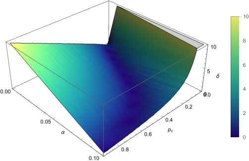
The distances (Eq. 4) between the true density and the detected density for each pair of and are shown in Fig. 3. For some values of the distance is negligible, which means the detected node degree is almost identical to the true node degree. The optimal , i.e. the one with the smallest distance between true density and detected density, depends on .
To have a general result for the optimal choice of when estimating a network characteristic of a given network topology, we sum over to marginalise out the influence of for each . We call this integrated quantity the total distance , i.e.
| (6) |
To identify the optimal choice of , we are interested in finding where the minimum of the total distance is located. Figure 4 shows for the example of the node degree of Erdős-Rényi networks. In this example, the minimum of is located at . This suggests that in order to optimally reconstruct the node degree of an Erdős-Rényi network should be chosen, which is close to the standard choice of but distinctively smaller.

3 Results
We applied our analysis to Erdős-Rényi, Watts-Strogatz and Barabási-Albert networks. For each network topology, we investigated four different network characteristics: node degree, number of links, global clustering coefficient and efficiency. The distance , which depends on both and the parameter of the network topology ( or ) is presented as density plot for all the investigated characteristics and network topologies in Fig. 5. All 12 investigated scenarios show a dependence of the distance on the choice of , suggesting that an optimum exists. For some scenarios, in particular node degree and number of links for Watts-Strogatz and Barabási-Albert networks, dependence of the distance on the parameter ( or ) is negligible. For other scenarios such as the global clustering coefficient in Watts-Strogatz networks the question arises if marginalising out the influence of is distorting the results. Detailed results for each network topology are presented below.
| Erdős-Rényi networks | Barabási-Albert networks | Watts-Strogatz networks | ||
| node degree |

|

|

|
|
| number of links |

|

|

|
|
| efficiency |

|

|

|
|
| global clustering coefficient |

|

|

|
|
For Erdős-Rényi networks of , , and nodes we varied from to in steps of . Figure 2 shows an example of some of these values in steps of . The results of the total distance for the node degree of Erdős-Rényi networks are shown in Fig. 4. The minimum of is located at (). For the remaining network characteristics, the Erdős-Rényi networks also show a clear minimum of the total distance in dependence on . The specific values of for the respective minimal total distances however vary; they are summarised in Table 1. The optimal for efficiency is noticeably smaller than for the other network characteristics. Moreover, we chose a broad range for to cover the broad spectrum of Erdős-Rényi networks. Marginalising out the dependence of the distance on may therefore be distorting our results (see also dependence on in Fig. 5). For a specific application we thus recommend narrowing the range of to values relevant for the application.
| Network Topology | ||||||
| and Characteristic | ||||||
| Erdős-Rényi: | ||||||
| node degree | 0.031 | 0.032 | 0.030 | 0.033 | 0.031 | 0.032 |
| number of links | 0.031 | 0.032 | 0.030 | 0.033 | 0.031 | 0.032 |
| global clustering coeff | 0.035 | 0.029 | 0.031 | 0.032 | 0.031 | 0.032 |
| efficiency | 0.016 | 0.063 | 0.012 | 0.083 | 0.020 | 0.050 |
| Barabási-Albert: | ||||||
| node degree | 0.018 | 0.056 | 0.012 | 0.083 | 0.007 | 0.143 |
| number of links | 0.018 | 0.056 | 0.012 | 0.083 | 0.007 | 0.143 |
| global clustering coeff | 0.024 | 0.042 | 0.021 | 0.048 | 0.019 | 0.053 |
| efficiency | 0.015 | 0.067 | 0.010 | 0.100 | 0.007 | 0.143 |
| Watts-Strogatz: | ||||||
| node degree | 0.009 | 0.111 | 0.007 | 0.143 | 0.004 | 0.250 |
| number of links | 0.009 | 0.111 | 0.007 | 0.143 | 0.004 | 0.250 |
| global clustering coeff | 0.008 | 0.125 | 0.006 | 0.167 | 0.004 | 0.250 |
| efficiency | 0.009 | 0.111 | 0.006 | 0.167 | 0.004 | 0.250 |
The set of Barabási-Albert networks of , , and nodes was chosen with average degree typical for networks in neuroscience (Papo et al., 2014; Stanley et al., 2013) by using parameters to varying in steps of . The total distances for the node degree of networks with nodes are shown in Fig. 6. The minimum is found for (), it is more pronounced than that for the Erdős-Rényi networks. Again, the other network characteristics and number of nodes all show a single minimum. The values for optimal and are summarised in Table 1. For this network topology a noticeably different optimal value for was found for the clustering coefficient.


Finally, we considered a set of Watts-Strogatz networks of , , and nodes with parameter varied between and in steps of . We analysed distances between the distributions of the node degree, the number of links, the global clustering coefficient and the efficiency. The minimum of the total distance for the node degree of networks with nodes is found for (). The total distances between node degree distributions for these networks are shown in Fig. 7. For all four characteristics and different values of clear minima can be identified and the values for optimal are similar (Table 1). The results for the efficiency however have to be interpreted with case as the distance showed a clear dependence on the parameter (see Fig. 5).
4 Discussion
We consider three topologies of networks Erdős-Rényi, Watts-Strogatz, and Barabási-Albert. For each topology, and for a specific characteristic, e.g. the node degree distribution, the number of links, the efficiency or global clustering coefficient, the rate of false positive and false negative conclusions about links can be optimally chosen in order to have less biased reconstruction.
For Erdős-Rényi networks, the values for identified with our method are close to standard choice of of . Standard alpha values are suboptimal when the topology of network is different. For the set of Barabási-Albert networks we found that the value for and consequently yields the most reliable results of the node degree. In this case, standard alpha values lead to a bigger distance between distributions of the node degree. The Watts-Strogatz networks yield the most reliable results for an even smaller value for and consequently . Moreover, for the optimal choice of the corresponding is rather high. This shows that the reliability of detecting individual false negative links in a network is less important than failing to recognise false positive links when network characteristics are estimated. Accepting a high rate of false negative links may thus be required when the aim is to infer a specific network characteristic.
This work shows that the standard choice of of is not optimal when the aim is to reconstruct the entire network topology. Moreover, needs to be adjusted depending on specific network topologies and characteristics. For example, consider Erdős-Rényi networks with and assume the relationship between and is Eq. 5. As result of 200 simulations, the mean of the node degree distribution of the original network is 11 and the mean for estimation using is 15. Choosing results in a mean of the node degree distribution of 13. The choice of is motivated by the assumption that the original network is known to be an Erdős-Rényi network with unknown parameter , see Table 1. For the same study, when the aim is to infer the efficiency , we calculate for the true network, for the one with , and when . The more we know about the network we want to infer the more accurate the reconstruction is since the simulation study can be tuned accordingly.
As mentioned in Section 2.2, the relationship between and depends on the number of data points , therefore the values of and leading to the minimal distance will change for different values of . Nevertheless, the results will remain qualitatively the same.
The size of the network, i.e. the number of nodes, also influences the result. The number of false positive and false negative conclusions about the presence of links depends on the number of total links in the network. Keeping the same rate of and and increasing, for example, the size of the network, leads to larger number of false positive and false negative detections of links. As shown in Table 1, for Erdős-Rényi networks the values of and leading to the minimal distance almost do not change. The reason is that the number of links increases proportionally with the number of nodes for each . This does not happen for Barabási-Albert and Watts-Strogatz networks; the values of leading to the minimal distance present a decreasing trend because of their constructions.
We considered the node degree distribution, the number of links, the efficiency, and the global clustering coefficient as example characteristics to show that the results depend on the characteristic under investigation. Nevertheless, our approach can be readily applied to other characteristics, as well as other network topologies.
5 Conclusion
False conclusions about the presence of links in a network typically alter network characteristics, such as the node degree distribution, the number of links, the global clustering coefficient and the efficiency. Identification of the underlying network topology relies on these characteristics and is thus hindered by false conclusions about links as well. For these reasons, the analysis of false positive and false negative conclusions about links is of key importance.
In this manuscript, assuming to know the underlying network topology, we investigate the influence of false positive and false negative conclusions about links in a network. We show that the values of and leading to minimal distance (difference in mean values) between the true network and the biased one change depending not only on the network topology, but also on the network characteristic of interest. Therefore, in the Inverse Problem, when the challenge is to infer the network topology from data, different values for and might be favourable when estimating different characteristics. We speculate that our simulation study can be used as an iterative procedure to achieve a better network reconstruction. Namely, when the network topology is not known a priori, various values for can be chosen to perform the first iteration step of the network reconstruction. The result of this first step gives an idea of the network topology we want to infer. For the second iteration step the value for can be adjusted according to the findings of the first step. This procedure can be iterated using the simulation study that we suggest in this paper in each iteration step, ultimately leading to a reconstruction of the network tailored to its previously unknown network topology.
This result suggests that in the Neurosciences, as well as in other scientific fields, various values for statistical inference could be considered within a simulation study to determine the optimal for the network characteristic of interest. If several network characteristics are of interest, it may be useful to adjust the value of for each characteristic.
Acknowledgements
This project has received funding from the European Union’s Horizon 2020 research and innovation programme under the Marie Sklodowska-Curie grant agreement No 642563.
The authors declare no competing financial interests.
References
- Barabási and Albert (1999) Barabási, A.-L., Albert, R., 1999. Emergence of scaling in random networks. Science 286, 509–512.
- Barabási and Pósfai (2016) Barabási, A.-L., Pósfai, M., 2016. Network science. Cambridge University Press, Cambridge.
- Bialonski et al. (2010) Bialonski, S., Horstmann, M.-T., Lehnertz, K., 2010. From brain to earth and climate systems: Small-world interaction networks or not? Chaos 20, 013134.
- Bialonski et al. (2011) Bialonski, S., Wendler, M., Lehnertz, K., 2011. Unraveling spurious properties of interaction networks with tailored random networks. PLoS ONE 6, 1–13.
- Bullmore and Sporns (2009) Bullmore, E., Sporns, O., 2009. Complex brain networks: graph theoretical analysis of structural and functional systems. Nat. Rev. Neurosci. 10, 186–198.
- Chavez et al. (2010) Chavez, M., Valencia, M., Latora, V., Martinerie, J., 2010. Complex networks: new trends for the analysis of brain connectivity. Int. J. Bifurcation Chaos 20 (06), 1677–1686.
- De Vico Fallani et al. (2014) De Vico Fallani, F., Richiardi, J., Chavez, M., Achard, S., 2014. Graph analysis of functional brain networks: practical issues in translational neuroscience. Philos. T. R. Soc. B 369 (1653).
- Devore (2011) Devore, J., 2011. Probability and Statistics for Engineering and the Sciences. Cengage Learning.
- Elsegai et al. (2015) Elsegai, H., Shiells, H., Thiel, M., Schelter, B., 2015. Network inference in the presence of latent confounders: The role of instantaneous causalities. J. Neurosci. Meth. 245, 91–106.
- Erdős and Rényi (1959) Erdős, P., Rényi, A., 1959. On random graphs. Publ. Math-Debrecen 6, 290–297.
- Erdős and Rényi (1960) Erdős, P., Rényi, A., 1960. On the evolution of random graphs. In: Publication of the Mathematical Institute of the Hungarian Academy of Sciences. pp. 17–61.
- Guo et al. (2008) Guo, S., Seth, A. K., Kendrick, K. M., Zhou, C., Feng, J., 2008. Partial Granger causality-Eliminating exogenous inputs and latent variables. J. Neurosci. Meth. 172, 79–93.
- Honey et al. (2007) Honey, C. J., Kötter, R., Breakspear, M., Sporns, O., 2007. Network structure of cerebral cortex shapes functional connectivity on multiple time scales. Proc. Natl. Acad. Sci. 104 (24), 10240–10245.
- Jalili and Knyazeva (2011) Jalili, M., Knyazeva, M. G., 2011. Constructing brain functional networks from eeg: partial and unpartial correlations. J. Integr. Neurosci. 10 (02), 213–232.
- Mader et al. (2015) Mader, W., Mader, M., Timmer, J., Thiel, M., Schelter, B., 2015. Networks: On the relation of bi- and multivariate measures. Sci. Rep. 5, 10805.
- Menezes et al. (2017) Menezes, M. B. C., Kim, S., Huang, R., 06 2017. Constructing a watts-strogatz network from a small-world network with symmetric degree distribution. PLoS One 12 (6), 1–9.
- Nalatore et al. (2007) Nalatore, H., Ding, M., Rangarajan, G., 2007. Mitigating the effects of measurement noise on Granger causality. Phys. Rev. E 75, 1–10.
- Newbold (1978) Newbold, P., 1978. Feedback induced by measurement errors. Int. Econ. Rev. 19, 787–791.
- Newman (2010) Newman, M., 2010. Networks: An Introduction. Oxford University Press, Inc., New York, NY, USA.
- Newman (2002) Newman, M. E. J., 2002. Random graphs as models of networks. In: Bornholdt, S., Schuster, H. G. (Eds.), Handbook of Graphs and Networks: From the Genome to the Internet. No. 1. pp. 34–68.
- Newman (2003) Newman, M. E. J., 2003. The structure and function of complex networks. SIAM Rev 45, 167–256.
- Olbrich et al. (2010) Olbrich, E., Kahle, T., Bertschinger, N., Ay, N., Jost, J., 2010. Quantifying structure in networks. Eur. Phys. J. B 77, 239–247.
- Papo et al. (2014) Papo, D., Buldu, J., Boccaletti, S., 2014. Network theory in neuroscience. Encyclopedia of Computational Neuroscience, 1852–1868.
- Pessoa (2014) Pessoa, L., 2014. Understanding brain networks and brain organization. Phys. Life Rev. 11, 400–435.
- Petersen and Sporns (2015) Petersen, S. E., Sporns, O., 2015. Brain Networks and Cognitive Architectures. Neuron 88, 207–219.
- Quinn and Keough (2002) Quinn, G., Keough, M., 2002. Experimental Design and Data Analysis for Biologists. Cambridge University Press.
- Ramb et al. (2013) Ramb, R., Eichler, M., Ing, A., Thiel, M., Weiller, C., Grebogi, C., Schwarzbauer, C., Timmer, J., Schelter, B., 2013. The impact of latent confounders in directed network analysis in neuroscience. Philos. T. Roy. Soc. A 371, 20110612.
- Schinkel et al. (2011) Schinkel, S., Zamora-López, G., Dimigen, O., Sommer, W., Kurths, J., 2011. Functional network analysis reveals differences in the semantic priming task. J. Neurosci. Meth. 197 (2), 333 – 339.
- Sommerlade et al. (2015) Sommerlade, L., Thiel, M., Mader, M., Mader, W., Timmer, J., Platt, B., Schelter, B., 2015. Assessing the strength of directed influences among neural signals: An approach to noisy data. J. Neurosci. Meth. 239, 47–64.
- Sporns et al. (2004) Sporns, O., Chialvo, D. R., Kaiser, M., Hilgetag, C. C., 2004. Organization, development and function of complex brain networks. Trends Cogn. Sci. 8, 418–425.
- Stanley et al. (2013) Stanley, M., Moussa, M., Paolini, B., Lyday, R., Burdette, J., Laurienti, P., 2013. Defining nodes in complex brain networks. Frontiers in Computational Neuroscience 7, 169.
- Watts (1999) Watts, D., 1999. Small Worlds: The Dynamics of Networks Between Order and Randomness. Princeton studies in complexity. Princeton University Press.
- Watts and Strogatz (1998) Watts, D. J., Strogatz, S. H., 1998. Collective dynamics of ’small-world’ networks. Nature 393, 440–442.
- Zerenner et al. (2014) Zerenner, T., Friederichs, P., Lehnertz, K., Hense, A., 2014. A gaussian graphical model approach to climate networks. Chaos 24, 023103.