跳到论文正文
W Papers独立论文阅读器 arXiv:1806.09869 论文正文 计算阅读时间 · 0%
引用这篇论文根据当前论文元数据生成,正式投稿前建议核对。


License: arXiv.org perpetual non-exclusive license
arXiv:1806.09869v1 [cs.IT] 26 Jun 2018

New extension constructions of optimal frequency hopping sequence setsThanks: This work is supported by the National Science Foundation of China(Grant No. 61401369), the Youth Science and Technology Fund of Sichuan Province(No.2017JQ0059)

Abstract.

In this paper, a general framework of constructing optimal frequency hopping sequence (FHS) sets is presented based on the designated direct product. Under the framework, we obtain infinitely many new optimal FHS sets by combining a family of sequences that are newly constructed in this paper with some known optimal FHS sets. Our constructions of optimal FHS sets are also based on extension method. However, our constructions remove the constraint requiring that the extension factor is co-prime with the length of original FHSs and get new parameters. In literature, most of the extension constructions suffer from this constraint. As a result, our constructions allow a great flexibility of choosing parameters of FHS sets for a given frequency-hopping spread spectrum system.
Keywords. Frequency hopping sequences, Optimal Hamming correlation, Extension construction.

Xianhua Niu

School of Computer and Software Engineering

Xihua University

National Key Laboratory of Science and Technology on Communications

University of Electronic Science and Technology of China

Chengdu, China.

Chaoping Xing

Division of Mathematical Sciences

School of Physical and Mathematical Sciences

Nanyang Technological University

Singapore.

1. Introduction

Frequency hopping (FH) multiple-access (MA) spread spectrum systems, with its anti-jamming, secure and multiple access properties, have found many applications in military radio communications, mobile communications, modern radar and sonar echolocation systems [1, 2]. In such systems, multiple frequency-shift keying (MFSK) is the data modulation technique employed, and wideband signals are generated by hopping from one frequency slot to anther over a large number of frequency slots. The frequency slots used are chosen pseudo-randomly by a code called frequency hopping sequence (FHS). As is often the case, in a multiple access environment, an important requirement is to keep the mutual interference between transmitters on a level as low as possible. This mutual interference occurs when two or more sources transmit the same frequency slot at the same time. The degree of the mutual interference is clearly related to the Hamming correlation properties of the frequency hopping sequences [1, 3]. In order to improve their performance, it is desirable to employ frequency hopping sequences (FHSs) having low Hamming correlation to reduce the multiple-access interference (also called hits) of frequencies [4]. Thus, the design of an FHS set with good property is an important problem.

The main purpose of FHS design is to find an FHS or an FHS set which is optimal under a given condition. In general, the optimality of an FHS set is measured by the Peng-Fan bound [5], whereas that of a single FHS is by the Lempel-Greenberger bound [4]. There are several algebraic or combinatorial constructions for optimal FHSs or FHS sets in the literature [6]-[22]. Moreover, some extension methods have been proposed [23]-[26], which generate several new families of optimal FHSs. By applying some known FHS sets, the existing extension constructions have produced new FHS sets with some desirable parameters. However, most of the extension constructions suffer from the constraint that the extension factor is co-prime with the length of original FHS sets.

In this paper, we present a general framework of constructing optimal FHS sets based on the designated direct product. Under the framework, we obtain infinitely many new optimal FHS sets which increase the length and alphabet size of the original FHS set by using flexible extension factor, but preserve its maximum Hamming correlation, as summarized in Table 1. Moreover, new constructions remove the constraint requiring that the extension factor is co-prime with the length of original FHSs. As a result, we have a great flexibility of choosing parameters of FHS sets for a given frequency-hopping spread spectrum system.

Table 1. The Extended FHS Set From a (N,v,λ,M)(N,v,\lambda;M) -FHS Set 𝒳\mathcal{X}.
Extended FHS set Constraints References Remarks
(n​N,n​v,λ,M)(nN,nv,\lambda;M)
m⁡(𝒳)≤lpf⁡(n)−1m(\mathcal{X})\leq{\rm lpf}(n)-1, gcd⁡(n,N)=1\gcd(n,N)=1.
[25][26]
(n​N,n​v,λ,M)(nN,nv,\lambda;M)
m⁡(𝒳)≤lpf⁡(n)−1m(\mathcal{X})\leq{\rm lpf}(n)-1.
Corollary 1 co-prime condition is removed
((q−1)​N,q​v,λ,M)((q-1)N,qv,\lambda;M)
m⁡(𝒳)≤qm(\mathcal{X})\leq q, gcd⁡((q−1),N)=1\gcd((q-1),N)=1.
[25][26]
((q−1)​N,q​v,λ,M)((q-1)N,qv,\lambda;M)
m⁡(𝒳)≤qm(\mathcal{X})\leq q.
Corollary 3 co-prime condition is removed
(d​N,q​v,λ,M)(dN,qv,\lambda;M)
m⁡(𝒳)≤pm(\mathcal{X})\leq p, d=(p−1)​pa−1d=(p-1)p^{a-1}.
Theorem 2 different parameter regime
(n⁡(q−1)​N,n​q​v,λ,M)(n(q-1)N,nqv,\lambda;M)
m⁡(𝒳)≤min⁡{lpf⁡(n)−1,q}m(\mathcal{X})\leq\min\{{\rm lpf}(n)-1,q\}, gcd⁡(n,N)=1\gcd(n,N)=1,
gcd⁡((q−1),N)=gcd⁡((q−1),n)=1\gcd((q-1),N)=\gcd((q-1),n)=1.
[25][26]
(n⁡(q−1)​N,n​q​v,λ,M)(n(q-1)N,nqv,\lambda;M)
m⁡(𝒳)≤min⁡{lpf⁡(n)−1,q}m(\mathcal{X})\leq\min\{{\rm lpf}(n)-1,q\}.
Corollary 5 co-prime condition is removed
(n​d​N,n​q​v,λ,M)(ndN,nqv,\lambda;M)
m⁡(𝒳)≤min⁡{lpf⁡(n)−1,p}m(\mathcal{X})\leq\min\{{\rm lpf}(n)-1,p\},
d=(p−1)​pa−1d=(p-1)p^{a-1}.
Corollary 4 different parameter regime

In Table 1, lpf⁡(n){\rm lpf}(n) denotes the least prime factor of nn, m⁡(𝒳)m(\mathcal{X}) denotes the maximum number of appearance of frequency slot in FHS set 𝒳\mathcal{X} and q=paq=p^{a} for a prime pp.

The rest of this paper is organized as follows. In Section 2, we give some preliminaries to FHSs. In Section 3, we present a general framework to construct optimal FHS sets based on the designated direct product. In Section 4, we obtain the new construction of optimal FHS sets with length n​NnN. In Section 5, we give a construction of optimal FHS sets with new parameter of length d​NdN or n​d​NndN. Finally, we conclude the paper in Section 6.

2. Preliminaries

Throughout this paper, the following notations will be used:

p1,…,pr:p_{1},\ldots,p_{r}: primes with p1<…<prp_{1}<\ldots<p_{r};

q1:q_{1}: power of prime p1p_{1};

q:q: power of prime pp;

⟨x⟩y:\langle x\rangle_{y}: the least nonnegative residue of xx modulo yy for an integer xx and a positive integer yy;

ℤn:\mathbb{Z}_{n}: the ring of integers modulo nn for a positive integer n>1n>1;

ord⁡(g):{\rm ord}(g): the multiplicative order of g∈ℤn∗g\in\mathbb{Z}_{n}^{*};

⌈z⌉:\lceil z\rceil: the largest integer less than or equal to zz;

(N,v,λ):(N,v,\lambda): an FHS of length NN over a frequency slot set of size vv, with the maximum Hamming autocorrelation λ\lambda;

(N,v,λ,M):(N,v,\lambda;M): an FHS set of MM sequences of length NN over a frequency slot set of size vv, with the maximum Hamming correlation λ\lambda.

Let ℱ={f1,f2,…,fv}\mathcal{F}=\{f_{1},f_{2},\ldots,f_{v}\} be a frequency slot set with size |ℱ|=v|\mathcal{F}|=v, 𝒳\mathcal{X} be a set of MM FHSs of length NN. For any two FHSs 𝐱i=(xi​(0),xi​(1),…,xi​(N−1)){\bf x}_{i}=\left(x_{i}(0),x_{i}(1),\ldots,x_{i}(N-1)\right), 𝐱j=(xj​(0),xj​(1),…,xj​(N−1))∈𝒳{\bf x}_{j}=\left(x_{j}(0),x_{j}(1),\ldots,x_{j}(N-1)\right)\in\mathcal{X}, 0≤i≠j≤M−10\leq i\neq j\leq M-1, the Hamming correlation function H𝐱i​𝐱j​(τ)H_{{\bf x}_{i}{\bf x}_{j}}(\tau) of sequences 𝐱i{\bf x}_{i} and 𝐱j{\bf x}_{j} at time delay τ\tau is defined as follows:

(1) H𝐱i​𝐱j​(τ)=∑t=0N−1h⁡(xi​(t),xj​(⟨t+τ⟩N)),0≤τ≤N−1,H_{{\bf x}_{i}{\bf x}_{j}}(\tau)=\sum^{N-1}_{t=0}h\left(x_{i}(t),x_{j}(\langle t+\tau\rangle_{N})\right),~~0\leq\tau\leq N-1,

where h⁡(a,b)=1h(a,b)=1 if a=ba=b, and h⁡(a,b)=0h(a,b)=0 otherwise. And only positive time shifts are considered.

For any given FHS set 𝒳\mathcal{X}, the maximum Hamming autocorrelation Ha​(𝒳)H_{a}(\mathcal{X}), the maximum Hamming crosscorrelation Hc​(𝒳)H_{c}(\mathcal{X}) and the maximum Hamming correlation Hm​(𝒳)H_{m}(\mathcal{X}) are defined as follows, respectively:

Ha​(𝒳)\displaystyle H_{a}(\mathcal{X}) =\displaystyle= max0<τ<N⁡{H𝐱i​𝐱i​(τ):𝐱∈𝒳},\displaystyle\max\limits_{0<\tau<N}\left\{H_{{\bf x}_{i}{\bf x}_{i}}(\tau):~{\bf x}\in\mathcal{X}\right\},
Hc​(𝒳)\displaystyle H_{c}(\mathcal{X}) =\displaystyle= max0≤τ<N{H𝐱i​𝐱j(τ):𝐱i,𝐱j∈𝒳,i≠j}.\displaystyle\max\limits_{0\leq\tau<N}\left\{H_{{\bf x}_{i}{\bf x}_{j}}(\tau):~{\bf x}_{i},{\bf x}_{j}\in\mathcal{X},i\neq j\right\}.
Hm​(𝒳)\displaystyle H_{m}(\mathcal{X}) =\displaystyle= max⁡{Ha​(𝒳),Hc​(𝒳)}.\displaystyle\max\left\{H_{a}(\mathcal{X}),H_{c}(\mathcal{X})\right\}.

In 2004, Peng and Fan [5] established the following bound of an FHS set.

Lemma 1 (Peng-Fan bound).

Let 𝒳\mathcal{X} be an FHS set of MM sequences and length NN over a given frequency slot set ℱ\mathcal{F} of size vv, we have

(2) Hm​(𝒳)≥⌈(M​N−v)​N(M​N−1)​v⌉.H_{m}(\mathcal{X})\geq\left\lceil\frac{(MN-v)N}{(MN-1)v}\right\rceil.

An (N,v,λ,M)(N,v,\lambda;M) FHS set 𝒳\mathcal{X} is called optimal if the Peng-Fan bound in Lemma 2 is met with equality. An (N,v,λ)(N,v,\lambda) FHS 𝐱{\bf x} is called optimal if the Lempel-Greenberger bound is met with equality.

In practical applications, the required length and alphabet size of an FHS or an FHS set are variable according to the specification of a given system or environment. Thus, it is very important to select optimal FHSs or FHS sets with flexible parameters under the given condition.

Lemma 2.

Let 𝒳={𝐱i=(xi​(0),xi​(1),…,xi​(N−1)):0≤i≤M−1}\mathcal{X}=\left\{{\bf x}_{i}=(x_{i}(0),x_{i}(1),\ldots,x_{i}(N-1)):0\leq i\leq M-1\right\} be an FHS set over frequency slot set ℱ={f1,f2,…,fv}\mathcal{F}=\{f_{1},f_{2},\ldots,f_{v}\}. For any fk∈ℱf_{k}\in\mathcal{F}, let

Φk={(i,a)|xi​(a)=fk},1≤k≤v.\Phi_{k}=\{(i,a)|x_{i}(a)=f_{k}\},1\leq k\leq v.

Then, the maximum number of appearance of any frequency slot fk∈ℱf_{k}\in\mathcal{F} in FHS set 𝒳\mathcal{X}, denoted by m⁡(𝒳)m(\mathcal{X}), can be written as m⁡(𝒳)=max1≤k≤v⁡{∣Φk∣:fk∈ℱ}m(\mathcal{X})=\max\limits_{1\leq k\leq v}\left\{\mid\Phi_{k}\mid:f_{k}\in\mathcal{F}\right\}.

In the following section, a framework based on the designated direct product will be given, which can be used to construct optimal FHS sets with new parameters.

3. A General Framework of Extension construction of FHS set

In this section, we give a framework of extension construction of FHS set based on the designated direct product by combining a family of sequences with some known optimal FHS sets.

For a (N,v,λ,M)(N,v,\lambda;M) FHS set 𝒳={𝐱i:0≤i≤M−1}\mathcal{X}=\{{\bf x}_{i}:0\leq i\leq M-1\} over ℱ\mathcal{F}, with

𝐱i=(xi​(0),xi​(1),…,xi​(N−1)).{\bf x}_{i}=(x_{i}(0),x_{i}(1),\ldots,x_{i}(N-1)).

Let ℰ={𝐞δ:0≤δ≤l−1}\mathcal{E}=\{{\bf e}_{\delta}:0\leq\delta\leq l-1\} be a sequence set of length nn over ℤm\mathbb{Z}_{m} with

𝐞δ=(eδ​(0),eδ​(1),…,eδ​(n−1)).{\bf e}_{\delta}=(e_{\delta}(0),e_{\delta}(1),\ldots,e_{\delta}(n-1)).

If m⁡(𝒳)≤lm(\mathcal{X})\leq l, let ωi​(t2)\omega_{i}(t_{2}) be a function with ωi​(t2)=φfk​(i,t2)\omega_{i}(t_{2})=\varphi_{f_{k}}(i,t_{2}), where φfk\varphi_{f_{k}} is a injective function from Φk\Phi_{k} to Zl∗Z_{l}^{*} for every kk with 0≤k≤v0\leq k\leq v, 0≤i≤M−10\leq i\leq M-1, 0≤t2≤N−10\leq t_{2}\leq N-1, the set Φk\Phi_{k} is defined as Lemma 2.

Then, an n×Nn\times N matrix is formed by combining the sequence 𝐞ωi​(t2){\bf e}_{\omega_{i}(t_{2})} with the FHS 𝐱i{\bf x}_{i} as follows:

𝐮i\displaystyle\small\ \ \ {\bf u}_{i}\!\! =\displaystyle\!\!=\!\! ((eωi​(0)​(0),xi​(0))(eωi​(1)​(0),xi​(1))…(eωi​(N−1)​(0),xi​(N−1))(eωi​(0)​(1),xi​(0))(eωi​(1)​(1),xi​(1))…(eωi​(N−1)​(1),xi​(N−1))⋮⋮⋱⋮(eωi​(0)​(n−1),xi​(0))(eωi​(1)​(n−1),xi​(1))…(eωi​(N−1)​(n−1),xi​(N−1)))\displaystyle\!\!\left({\begin{array}[]{*{20}{c}}{\left(e_{\omega_{i}(0)}(0),x_{i}(0)\right)}&{\left(e_{\omega_{i}(1)}(0),x_{i}(1)\right)}&\ldots&{\left(e_{\omega_{i}(N-1)}(0),x_{i}(N-1)\right)}\\ {\left(e_{\omega_{i}(0)}(1),x_{i}(0)\right)}&{\left(e_{\omega_{i}(1)}(1),x_{i}(1)\right)}&\ldots&{\left(e_{\omega_{i}(N-1)}(1),x_{i}(N-1)\right)}\\ \vdots&\vdots&\ddots&\vdots\\ {\left(e_{\omega_{i}(0)}(n-1),x_{i}(0)\right)}&{\left(e_{\omega_{i}(1)}(n-1),x_{i}(1)\right)}&\ldots&{\left(e_{\omega_{i}(N-1)}(n-1),x_{i}(N-1)\right)}\\ \end{array}}\right)
=\displaystyle\!\!=\!\! (ui​(0)ui​(1)…ui​(N−1)ui​(N)ui​(N+1)…ui​(2​N−1)⋮⋮⋱⋮ui​((n−1)​N)ui​((n−1)​N+1)…ui​(n​N−1)).\displaystyle\!\!\left({\begin{array}[]{*{20}{c}}{{u_{i}(0)}}&{{u_{i}(1)}}&\ldots&{{u_{i}(N-1)}}\\ {{u_{i}(N)}}&{{u_{i}(N+1)}}&\ldots&{{u_{i}(2N-1)}}\\ \vdots&\vdots&\ddots&\vdots\\ {{u_{i}((n-1)N)}}&{{u_{i}((n-1)N+1)}}&\ldots&{{u_{i}(nN-1)}}\\ \end{array}}\right).

By reading the elements in 𝐮i{\bf u}_{i} row by row, we get an extended FHS 𝐮i=(ui​(0),ui​(1),…,ui​(n​N−1)){\bf u}_{i}=(u_{i}(0),u_{i}(1),\ldots,u_{i}(nN-1)) of period n​NnN. Thus, we can obtain the extended FHS set 𝒰={𝐮i:0≤i≤M−1}\mathcal{U}=\{{\bf u}_{i}:0\leq i\leq M-1\}, where the length nn of sequence 𝐞δ{\bf e}_{\delta} is called the extension factor. For short, we write the extended FHS 𝐮i{\bf u}_{i} as

𝐮i=E⁡[𝐞ωi,𝐱i]=E⁡[(𝐞ωi​(0),xi​(0)),(𝐞ωi​(1),xi​(1)),…,(𝐞ωi​(N−1),xi​(N−1))],{\bf u}_{i}=E\left[{\bf e}_{\omega_{i}},{\bf x}_{i}\right]=E\left[\left({\bf e}_{\omega_{i}(0)},x_{i}(0)\right),\left({\bf e}_{\omega_{i}(1)},x_{i}(1)\right),\ldots,\left({\bf e}_{\omega_{i}(N-1)},x_{i}(N-1)\right)\right],

where EE is the extension operator.

Another extended FHS 𝐮j{\bf u}_{j} can be generated by combining 𝐞ωj{\bf e}_{\omega^{j}} with 𝐱j{\bf x}_{j} as follows:

𝐮j=E⁡[𝐞ωj,𝐱j]=E⁡[(𝐞ωj​(0),xj​(0)),(𝐞ωj​(1),xj​(1)),…,(𝐞ωj​(N−1),xj​(N−1))].{\bf u}_{j}=E\left[{\bf e}_{\omega_{j}},{\bf x}_{j}\right]=E\left[\left({\bf e}_{\omega_{j}(0)},x_{j}(0)\right),\left({\bf e}_{\omega_{j}(1)},x_{j}(1)\right),\ldots,\left({\bf e}_{\omega_{j}(N-1)},x_{j}(N-1)\right)\right].

Consider its cyclical shift version L(τ)​(𝐮j)L^{(\tau)}({\bf u}_{j}), where LL is the (left cyclical) shift operator, τ=N​τ1+τ2\tau=N\tau_{1}+\tau_{2}, 0≤τ1≤n−10\leq\tau_{1}\leq n-1, 0≤τ2≤N−10\leq\tau_{2}\leq N-1. By the matrix representation, L(τ)​(𝐮j)L^{(\tau)}({\bf u}_{j}) could be written as

(13) ((eωj​(τ2)​(τ1),xj​(τ2))…(eωj​(N−1)​(τ1),xj​(N−1))…(eωj​(τ2−1)​(τ1),xj​(τ2−1))⋮⋮⋮⋱⋮(eωj​(τ2)​(n−1),xj​(τ2))…(eωj​(N−1)​(n−1),xj​(N−1))…(eωj​(τ2−1)​(n−1),xj​(τ2−1))(eωj​(τ2)​(0),xj​(τ2))…(eωj​(N−1)​(0),xj​(N−1))…(eωj​(τ2−1)​(0),xj​(τ2−1))⋮⋮⋮⋱⋮(eωj​(τ2)​(τ1−1),xj​(τ2))…(eωj​(N−1)​(τ1−1),xj​(N−1))…(eωj​(τ2−1)​(τ1−1),xj​(τ2−1))).\footnotesize\left({\begin{array}[]{*{20}{c}}{\left(e_{\omega_{j}(\tau_{2})}(\tau_{1}),x_{j}(\tau_{2})\right)}&\ldots&{\left(e_{\omega_{j}(N-1)}(\tau_{1}),x_{j}(N\!-\!1)\right)}&\ldots&{\left(e_{\omega_{j}(\tau_{2}-1)}(\tau_{1}),x_{j}(\tau_{2}\!-\!1)\right)}\\ \vdots&\vdots&\vdots&\ddots&\vdots\\ {\left(e_{\omega_{j}(\tau_{2})}(n\!-\!1),x_{j}(\tau_{2})\right)}&\ldots&{\left(e_{\omega_{\!j}(N-1)}(n-1),x_{j}(N\!-\!1)\right)}&\ldots&{\left(e_{\omega_{j}(\tau_{2}-1)}(n-1),x_{j}(\tau_{2}\!-\!1)\right)}\\ {\left(e_{\omega_{j}(\tau_{2})}(0),x_{j}(\tau_{2})\right)}&\ldots&{\left(e_{\omega_{\!j}(N-1)}(0),x_{j}(N\!-\!1)\right)}&\ldots&{\left(e_{\omega_{j}(\tau_{2}-1)}(0),x_{j}(\tau_{2}\!-\!1)\right)}\\ \vdots&\vdots&\vdots&\ddots&\vdots\\ {\left(e_{\omega_{j}(\tau_{2})}(\tau_{1}\!-\!1),x_{j}(\tau_{2})\right)}&\ldots&{\left(e_{\omega_{j}(N-1)}(\tau_{1}\!-\!1),x_{j}(N\!-\!1)\right)}&\ldots&{\left(e_{\omega_{j}(\tau_{2}-1)}(\tau_{1}\!-\!1),x_{j}(\tau_{2}\!-\!1)\right)}\\ \end{array}}\right).

Obviously, L(τ)​(𝐮j)L^{(\tau)}({\bf u}_{j}) is just another extended FHS. Namely, we have

L(τ)​(𝐮j)=E⁡[(L(τ1)​(𝐞ωj​(τ2)),xj​(τ2)),…,(L(τ1)​(𝐞ωj​(N−1)),xj​(N−1)),…,(L(τ1)​(𝐞ωj​(τ2−1)),xj​(τ2−1))].\footnotesize L^{(\tau)}\!({\bf u}_{j})=E\left[\left(L^{(\tau_{1})}({\bf e}_{\omega_{j}(\tau_{2})}),x_{j}(\tau_{2})\right),\ldots,\left(L^{(\tau_{1})}({\bf e}_{\omega_{j}(N-1)}),x_{j}(N-1)\right),\ldots,\left(L^{(\tau_{1})}({\bf e}_{\omega_{j}(\tau_{2}-1)}),x_{j}(\tau_{2}-1)\right)\right].

Then, the Hamming correlation function between the extended FHSs 𝐮i{\bf u}_{i} and 𝐮j{\bf u}_{j} at shift τ\tau becomes the following from (3) and (13), i.e.,

(14) H𝐮i​𝐮j​(τ)\displaystyle H_{{\bf u}_{i}{\bf u}_{j}}(\tau) =\displaystyle= ∑t2=0N−1(∑t1=0n−1h⁡(eωi​(t2)​(t1),(eωj​(t2+τ2)​(t1+τ1))))⋅h⁡(xi​(t2),xj​(t2+τ2))\displaystyle\sum\limits_{t_{2}=0}^{N-1}\left(\sum\limits_{t_{1}=0}^{n-1}h\left(e_{\omega_{i}(t_{2})}(t_{1}),(e_{\omega_{j}(t_{2}+\tau_{2})}(t_{1}+\tau_{1}))\right)\right)\cdot h\left(x_{i}(t_{2}),x_{j}(t_{2}+\tau_{2})\right)
=\displaystyle= ∑t2=0N−1(H𝐞ωi​(t2),𝐞ωi​(t2+τ2)​(τ1))⋅h⁡(xi​(t2),xj​(t2+τ2)).\displaystyle\sum\limits_{t_{2}=0}^{N-1}\left(H_{{\bf e}_{\omega_{i}(t_{2})},{\bf e}_{\omega_{i}(t_{2}+\tau_{2})}}(\tau_{1})\right)\cdot h\left(x_{i}(t_{2}),x_{j}(t_{2}+\tau_{2})\right).\
Lemma 3.

With the above notation, the nontrivial Hamming correlation between 𝐮i{\bf u}_{i} and 𝐮j{\bf u}_{j} is

H𝐮i​𝐮j​(τ)≤{N​Ha​(ℰ),i=j,τ2=0,τ1≠0,λ​Hm​(ℰ),i≠j​o​r​τ2≠0,\displaystyle H_{{\bf u}_{i}{\bf u}_{j}}(\tau)\leq\left\{{\begin{array}[]{*{20}{c}}NH_{a}(\mathcal{E}),&i=j,\tau_{2}=0,\tau_{1}\neq 0,\\ \lambda H_{m}(\mathcal{E}),&i\neq j\ or\ \tau_{2}\neq 0,\\ \end{array}}\right.

for any 0≤i,j≤M−1,0≤τ1≤n−1,0≤τ2≤N−10\leq i,j\leq M-1,0\leq\tau_{1}\leq n-1,0\leq\tau_{2}\leq N-1.

Proof.

Let τ=N​τ1+τ2\tau=N\tau_{1}+\tau_{2}, where 0≤τ1≤n−1,0≤τ2≤N−10\leq\tau_{1}\leq n-1,0\leq\tau_{2}\leq N-1. In order to compute H𝐮i​𝐮j​(τ)H_{{\bf u}_{i}{\bf u}_{j}}(\tau), we divide the problem into two cases.

Case OPENi)i). i=j,τ2=0i=j,\tau_{2}=0.

If τ1=0\tau_{1}=0, then

H𝐮i​𝐮i​(0)\displaystyle H_{{\bf u}_{i}{\bf u}_{i}}(0) =\displaystyle= ∑t2=0N−1n⋅1=n​N.\displaystyle\sum\limits_{t_{2}=0}^{N-1}n\cdot 1=nN.

This is a trivial case.

If τ1≠0\tau_{1}\neq 0, then

H𝐮i​𝐮i​(τ)\displaystyle H_{{\bf u}_{i}{\bf u}_{i}}(\tau) =\displaystyle= ∑t2=0N−1(H𝐞ωi​(t2),𝐞ωi​(t2)​(τ1))⋅1\displaystyle\sum\limits_{t_{2}=0}^{N-1}\left(H_{{\bf e}_{\omega_{i}(t_{2})},{\bf e}_{\omega_{i}(t_{2})}}(\tau_{1})\right)\cdot 1
=\displaystyle= ∑t2=0N−1(H𝐞ωi​(t2),𝐞ωi​(t2)​(τ1)).\displaystyle\sum\limits_{t_{2}=0}^{N-1}\left(H_{{\bf e}_{\omega_{i}(t_{2})},{\bf e}_{\omega_{i}(t_{2})}}(\tau_{1})\right).

Therefore, for i=j,τ2=0i=j,\tau_{2}=0

H𝐮i​𝐮i​(τ)={n​N,i​f​τ1=0,∑t2=0N−1(H𝐞ωi​(t2),𝐞ωi​(t2)​(τ1)),o​t​h​e​r​w​i​s​e.\displaystyle H_{{\bf u}_{i}{\bf u}_{i}}(\tau)=\left\{{\begin{array}[]{*{20}{c}}nN,&if\tau_{1}=0,\\ \sum\limits_{t_{2}=0}^{N-1}\left(H_{{\bf e}_{\omega_{i}(t_{2})},{\bf e}_{\omega_{i}(t_{2})}}(\tau_{1})\right),&otherwise.\\ \end{array}}\right.

So, we have H𝐮i​𝐮i​(τ)≤N​Ha​(ℰ)H_{{\bf u}_{i}{\bf u}_{i}}(\tau)\leq NH_{a}(\mathcal{E}) for i=j,τ2=0,τ1≠0i=j,\tau_{2}=0,\tau_{1}\neq 0.

Case OPENi​i)ii). i≠ji\neq j or τ2≠0\tau_{2}\neq 0.

In this case, based on the definition of ω\omega, we have ωi​(t2)≠ωj​(t2+τ2)\omega_{i}(t_{2})\neq\omega_{j}(t_{2}+\tau_{2}) if h⁡(xi​(t2),xj​(t2+τ2))=1h\left(x_{i}(t_{2}),x_{j}(t_{2}+\tau_{2})\right)=1. Thus, we can express the Hamming correlation of 𝒮\mathcal{S} by using the maximum Hamming correlation Hm​(ℰ)H_{m}(\mathcal{E}) of sequence set ℰ\mathcal{E} as

H𝐮i​𝐮j​(τ)\displaystyle H_{{\bf u}_{i}{\bf u}_{j}}(\tau) =\displaystyle= ∑t2=0N−1(H𝐞ωi​(t2),𝐞ωj​(t2+τ2)​(τ1))⋅h⁡(xi​(t2),xj​(t2+τ2))\displaystyle\sum\limits_{t_{2}=0}^{N-1}\left(H_{{\bf e}_{\omega_{i}(t_{2})},{\bf e}_{\omega_{j}(t_{2}+\tau_{2})}}(\tau_{1})\right)\cdot h\left(x_{i}(t_{2}),x_{j}(t_{2}+\tau_{2})\right)
≤\displaystyle\leq ∑t2=0N−1Hc​(ℰ)⋅h⁡(xi​(t2),xj​(t2+τ2))\displaystyle\sum\limits_{t_{2}=0}^{N-1}H_{c}(\mathcal{E})\cdot h\left(x_{i}(t_{2}),x_{j}(t_{2}+\tau_{2})\right)
≤\displaystyle\leq λ​Hc​(ℰ).\displaystyle\lambda H_{c}(\mathcal{E}).

By summarizing the results of Case OPENi)i) and Case OPENi​i)ii), we have

H𝐮i​𝐮j​(τ)≤{N​Ha​(ℰ),i=j,τ2=0,τ1≠0,λ​Hc​(ℰ),o​t​h​e​r​w​i​s​e.\displaystyle H_{{\bf u}_{i}{\bf u}_{j}}(\tau)\leq\left\{{\begin{array}[]{*{20}{c}}NH_{a}(\mathcal{E}),&i=j,\tau_{2}=0,\tau_{1}\neq 0,\\ \lambda H_{c}(\mathcal{E}),&otherwise.\\ \end{array}}\right.

∎

Lemma 4.

With the above notation, specially, the nontrivial Hamming correlation between 𝐮i{\bf u}_{i} and 𝐮j{\bf u}_{j} is

H𝐮i​𝐮j​(τ)​{=0,i=j,τ2=0,τ1≠0,≤λ,o​t​h​e​r​w​i​s​e,\displaystyle H_{{\bf u}_{i}{\bf u}_{j}}(\tau)\left\{{\begin{array}[]{*{20}{c}}=0,&i=j,\tau_{2}=0,\tau_{1}\neq 0,\\ \leq\lambda,&otherwise,\\ \end{array}}\right.

if the maximum Hamming autocorrelation and crosscorrelation of set ℰ\mathcal{E} satisfy Ha​(ℰ)=0H_{a}(\mathcal{E})=0 and Hc​(ℰ)=1H_{c}(\mathcal{E})=1.

For short, ℰ\mathcal{E} is called one-coincidence sequence set if the maximum Hamming autocorrelation and crosscorrelation of set ℰ\mathcal{E} satisfy Ha​(ℰ)=0H_{a}(\mathcal{E})=0 and Hc​(ℰ)=1H_{c}(\mathcal{E})=1.

Under this framework, two new constructions of FHS set will be presented in the following sections, from which infinitely many new optimal FHSs or FHS sets can be obtained. By choosing the one-coincidence sequence set ℰ\mathcal{E} and the existing optimal FHS sets 𝒳\mathcal{X} with different parameters, it is expected that there exist some more classes of optimal FHS sets which can be obtained from the our framework.

4. Optimal FHS Sets of Length n​NnN

In this section, we present a new design for optimal FHS set from any known optimal FHS set under the framework in Section 3.

Let ℱ={f1,f2,…,fv}\mathcal{F}=\{f_{1},f_{2},\ldots,f_{v}\} be a frequency slot set with size |ℱ|=v|\mathcal{F}|=v. Our procedure of the extension construction is described as follows.

Construction 1.

Construction of optimal FHS sets of length n​NnN.

  1. Step 1:

    Select an optimal (N,v,λ,M)(N,v,\lambda;M) FHS set

    𝒳={𝐱i=(xi​(0),xi​(1),…,xi​(N−1)):0≤i≤M−1}.\mathcal{X}=\left\{{\bf x}_{i}=(x_{i}(0),x_{i}(1),\ldots,x_{i}(N-1)):0\leq i\leq M-1\right\}.

    The maximum number of appearance of frequency slot in 𝒳\mathcal{X} is m⁡(𝒳)m(\mathcal{X}).

  2. Step 2:

    Let q1=p1a1q_{1}=p_{1}^{a_{1}} for a prime p1p_{1} and a positive integer a1a_{1}. Let g′g^{\prime} be a primitive element of ℤp1∗\mathbb{Z}^{*}_{p_{1}}, so g=g′g=g^{\prime} or g=g′+p1g=g^{\prime}+p_{1} is the primitive element of ℤq1∗\mathbb{Z}^{*}_{q_{1}}. Generate a set

    ℰ={𝐞j=(0⋅gj,1⋅gj,⋯,(q1−1)⋅gj):0≤j≤p1−2}.\mathcal{E}=\{{\bf e}_{j}=(0\cdot g^{j},1\cdot g^{j},\cdots,(q_{1}-1)\cdot g^{j}):0\leq j\leq p_{1}-2\}.
  3. Step 3:

    If m⁡(𝒳)≤p1−1m(\mathcal{X})\leq p_{1}-1, let ωi​(t2)\omega_{i}(t_{2}) be a function with ωi​(t2)=φfk​(i,t2)\omega_{i}(t_{2})=\varphi_{f_{k}}(i,t_{2}), where φfk\varphi_{f_{k}} is a injective function from Φk\Phi_{k} to Zl∗Z_{l}^{*} for every kk with 0≤k≤v0\leq k\leq v, 0≤i≤M−10\leq i\leq M-1, 0≤t2≤N−10\leq t_{2}\leq N-1, the set Φk\Phi_{k} is defined as Lemma 2.

  4. Step 4:

    We can construct the desired FHS set 𝒮={𝐬i:0≤i≤M−1}\mathcal{S}=\{{\bf s}_{i}:0\leq i\leq M-1\},

    𝐬i=I⁡[(𝐞ωi​(0),xi​(0)),(𝐞ωi​(1),xi​(1)),⋯,(𝐞ωi​(N−1),xi​(N−1))].{\bf s}_{i}=I\left[\left({\bf e}_{\omega_{i}(0)},x_{i}(0)),({\bf e}_{\omega_{i}(1)},x_{i}(1)),\cdots,({\bf e}_{\omega_{i}(N-1)},x_{i}(N-1)\right)\right].
Lemma 5.

The set ℰ\mathcal{E} in Construction 1 has the following properties:

(i)(i) ℰ\mathcal{E} is a sequence set with p1−1p_{1}-1 sequences of length q1q_{1} over ℤq1\mathbb{Z}_{q_{1}};

(i​i)(ii) Ha​(ℰ)=0H_{a}(\mathcal{E})=0, Hc​(ℰ)=1H_{c}(\mathcal{E})=1.

Proof.

It is easily checked that the sequence set ℰ\mathcal{E} in Construciton 1 is a set with p1−1p_{1}-1 sequences of length q1q_{1} over ℤq1\mathbb{Z}_{q_{1}}. For any 0≤j1,j2≤p1−20\leq j_{1},j_{2}\leq p_{1}-2, 0≤t≤q1−10\leq t\leq q_{1}-1, the Hamming correlation H𝐞j1​𝐞j2​(t)H_{{\bf e}_{j_{1}}{\bf e}_{j_{2}}}(t) between 𝐞j1{\bf e}_{j_{1}} and 𝐞j2{\bf e}_{j_{2}} is given by

H𝐞j1​𝐞j2​(t)\displaystyle H_{{\bf e}_{j_{1}}{\bf e}_{j_{2}}}(t) =\displaystyle= ∑i=0q1−1h⁡(⟨i​gj1⟩q1,⟨(i+t)​gj2⟩q1).\displaystyle\sum\limits_{i=0}^{q_{1}-1}h\left(\langle ig^{j_{1}}\rangle_{q_{1}},\langle(i+t)g^{j_{2}}\rangle_{q_{1}}\right).

In order to compute H𝐞j1​𝐞j2​(t)H_{{\bf e}_{j_{1}}{\bf e}_{j_{2}}}(t), we divide the problem into two cases.

Case OPENi)i). j1=j2j_{1}=j_{2}.

In this case, since gg is a primitive element of ℤq1∗\mathbb{Z}^{*}_{q_{1}}, we have i​gj1≠(i+t)​gj1modq1ig^{j_{1}}\neq(i+t)g^{j_{1}}\mod\ {q_{1}} if t≠0t\neq 0. Then, we can obtain that

H𝐞j1​𝐞j1​(t)={q1,t=0,0,o​t​h​e​r​w​i​s​e.\displaystyle H_{{\bf e}_{j_{1}}{\bf e}_{j_{1}}}(t)=\left\{{\begin{array}[]{*{20}{c}}q_{1},&t=0,\\ 0,&otherwise.\\ \end{array}}\right.

Case OPENi​i)ii). j1≠j2j_{1}\neq j_{2}.

Since g=g′g=g^{\prime} or g′+p1g^{\prime}+p_{1} is the primitive element ∈ℤq1∗\in\mathbb{Z}^{*}_{q_{1}}, where g′g^{\prime} is a primitive element ∈ℤp1∗\in\mathbb{Z}^{*}_{p_{1}}. Hence, for any 0≤j1,j2≤p1−20\leq j_{1},j_{2}\leq p_{1}-2, we let gθ≡gj1−gj2modq1g^{\theta}\equiv g^{j_{1}}-g^{j_{2}}\mod{q_{1}}, where 0≤θ≤ord⁡(q1)−10\leq\theta\leq{{\rm ord}(q_{1})-1}.

Then, we have

H𝐞j1​𝐞j2​(t)\displaystyle H_{{\bf e}_{j_{1}}{\bf e}_{j_{2}}}(t) =\displaystyle= ∑i=0q1−1h⁡(⟨i​gj1⟩q1,⟨(i+t)​gj2⟩q1)\displaystyle\sum\limits_{i=0}^{q_{1}-1}h\left(\langle ig^{j_{1}}\rangle_{q_{1}},\langle(i+t)g^{j_{2}}\rangle_{q_{1}}\right)
=\displaystyle= ∑i=0q1−1h⁡(⟨i​gθ⟩q1,⟨t​gj2⟩q1).\displaystyle\sum\limits_{i=0}^{q_{1}-1}h\left(\langle ig^{\theta}\rangle_{q_{1}},\langle tg^{j_{2}}\rangle_{q_{1}}\right).

Thus, we can obtain

H𝐞j1​𝐞j2​(t)=1.\displaystyle H_{{\bf e}_{j_{1}}{\bf e}_{j_{2}}}(t)=1.

since h⁡(⟨i​gθ⟩q1,⟨t​gj2⟩q1)=1h\left(\langle ig^{\theta}\rangle_{q_{1}},\langle tg^{j_{2}}\rangle_{q_{1}}\right)=1 only if i≡t​g(j2−θ)modq1i\equiv tg^{(j_{2}-\theta)}\mod{q_{1}}.

By summarizing the results of Case OPENi)i) and OPENi​i)ii), we have the nontrivial Hamming correlation of ℰ\mathcal{E} is

H𝐞j1​𝐞j2​(t)={0,j1=j2,t≠0,1,j1≠j2.\displaystyle H_{{\bf e}_{j_{1}}{\bf e}_{j_{2}}}(t)=\left\{{\begin{array}[]{*{20}{c}}0,&j_{1}=j_{2},t\neq 0,\\ 1,&j_{1}\neq j_{2}.\\ \end{array}}\right.

∎

Theorem 1.

The FHS set 𝒮\mathcal{S} constructed by Construction 1 is an optimal (q1​N,q1​v,λ,M)(q_{1}N,q_{1}v,\lambda;M) FHS set over ℤq1×ℱ\mathbb{Z}_{q_{1}}\times\mathcal{F} if ⌈(N​M−v)(N​M−1)​Nv⌉=⌈(q1​N​M−v)(q1​N​M−1)​Nv⌉\left\lceil{\frac{{(NM-v)}}{{(NM-1)}}\frac{N}{v}}\right\rceil=\left\lceil\frac{(q_{1}NM-v)}{(q_{1}NM-1)}\frac{N}{v}\right\rceil.

Proof.

It is easily checked that that the extended FHS set 𝒮\mathcal{S} in Construciton 1 is a set with MM sequences of length q1​Nq_{1}N over ℤq1×ℱ\mathbb{Z}_{q_{1}}\times\mathcal{F}.

From Lemma 3,we know that the Hamming correlation of FHS set 𝒮\mathcal{S} is based on the correlation of set ℰ\mathcal{E}. Thus, from Lemma 5, we can obtain that Hm​(𝒮)=Hm​(𝒳)=λH_{m}(\mathcal{S})=H_{m}(\mathcal{X})=\lambda.

Then, we verify the optimality of the extended FHS set 𝒮\mathcal{S}. Since the optimal FHS set 𝒳\mathcal{X} satisfies Peng-Fan bound [5], we have λ=⌈(N​M−v)(N​M−1)​Nv⌉\lambda=\left\lceil{\frac{{(NM-v)}}{{(NM-1)}}\frac{N}{v}}\right\rceil.

According to the Peng-Fan bound [5], the FHS set 𝒮\mathcal{S} with the sequence length q1​Nq_{1}N, the family size MM and the frequency slot set of size q1​vq_{1}v over ℤq1×ℱ\mathbb{Z}_{q_{1}}\times\mathcal{F}, the optimal maximum Hamming correlation Hm′H^{\prime}_{m} of 𝒮\mathcal{S} should be

Hm′≥⌈(M​q1​N−v)(M​q1​N−1)​q1​Nq1​v⌉=⌈(M​q1​N−v)(M​q1​N−1)​Nv⌉.\displaystyle{H^{\prime}_{m}}\geq\left\lceil\frac{(Mq_{1}N-v)}{(Mq_{1}N-1)}\frac{q_{1}N}{q_{1}v}\right\rceil=\left\lceil\frac{(Mq_{1}N-v)}{(Mq_{1}N-1)}\frac{N}{v}\right\rceil.

Thus, we have the FHS set 𝒮\mathcal{S} in Construction 1 is optimal if ⌈(q1​N​M−v)(q1​N​M−1)​Nv⌉=⌈(N​M−v)(N​M−1)​Nv⌉\left\lceil\frac{(q_{1}NM-v)}{(q_{1}NM-1)}\frac{N}{v}\right\rceil=\left\lceil{\frac{{(NM-v)}}{{(NM-1)}}\frac{N}{v}}\right\rceil. This constraint is easy to satisfy because q1​N​M>N​Mq_{1}NM>NM.

∎

The above construction remove the constraint requiring that the expansion factor is coprime with the length of original FHSs. Moreover, it is possible to extend the length of 𝒮\mathcal{S} by the extension factor q2=p2a2q_{2}=p^{a_{2}}_{2}, where a2a_{2} is a positive integer and p2p_{2} is a prime with p2>p1p_{2}>p_{1}. In this way, Construction 1 can be applied recursively infinitely many times. Since Construction 1 can be applied to any existing optimal FHSs or FHS sets, it is expected that there exist some more classes of optimal FHS sets which can be obtained from our construction.

Corollary 1.

For positive integers rr and a1,…,ara_{1},\ldots,a_{r}, let n=q1⋯qrn=q_{1}\cdots q_{r}, where qi=piai,1≤i≤rq_{i}=p^{a_{i}}_{i},1\leq i\leq r, p1,…,prp_{1},\ldots,p_{r} are primes with p1<…<prp_{1}<\ldots<p_{r}. If m⁡(𝒳)≤p1−1m(\mathcal{X})\leq p_{1}-1, then there exists an optimal (n​N,n​v,λ,M)(nN,nv,\lambda;M) FHS set over ℤqr×⋯×ℤq1×ℱ\mathbb{Z}_{q_{r}}\times\cdots\times\mathbb{Z}_{q_{1}}\times\mathcal{F}.

Construction 1 in the case of M=1M=1 leads to the construction of a new single FHS. Based on Construction 1, it is possible to obtain new optimal FHSs with respect to the Lempel-Greenberger bound.

Corollary 2.

Assume that there exists an optimal (N,v,λ)(N,v,\lambda)-FHS 𝐬{\bf s} with respect to the Lempel-Greenberger bound, defined over ℱ\mathcal{F}. For positive integers rr and a1,…,ara_{1},\ldots,a_{r}, let n=q1⋯qrn=q_{1}\cdots q_{r}, where qi=piai,1≤i≤rq_{i}=p^{a_{i}}_{i},1\leq i\leq r, p1,…,prp_{1},\ldots,p_{r} are primes with p1<…<prp_{1}<\ldots<p_{r}. If m⁡(𝐬)≤p1−1m({\bf s})\leq p_{1}-1, then there exists an optimal (n​N,n​v,λ)(nN,nv,\lambda) FHS over ℤqr×⋯×ℤq1×ℱ\mathbb{Z}_{q_{r}}\times\cdots\times\mathbb{Z}_{q_{1}}\times\mathcal{F}.

Remark 1.

By means of our method, Chung’s Construction A in [25] is a special case of Corollary 1 for gcd⁡(n,N)=1\gcd(n,N)=1 and ωi​(t2)=∑α=0i−1∑t=0N−1h⁡(xα​(t),xi​(t2))+∑β=0t2−1h⁡(xi​(β),xi​(t2))−1\omega_{i}(t_{2})=\sum^{i-1}_{\alpha=0}\sum^{N-1}_{t=0}h(x_{\alpha}(t),x_{i}(t_{2}))+\sum^{t_{2}-1}_{\beta=0}h(x_{i}(\beta),x_{i}(t_{2}))-1 for any 0≤i≤M−1,0≤t2≤N−10\leq i\leq M-1,0\leq t_{2}\leq N-1.

Example 1.

We select an optimal (26,7,4,3)(26,7,4;3) FHS set 𝒳={𝐱0,𝐱1,𝐱2}\mathcal{X}=\{{\bf x}_{0},{\bf x}_{1},{\bf x}_{2}\} over ℤ7\mathbb{Z}_{7} , such that

𝐱0={6,1,5,3,4,4,1,2,3,5,2,0,0,6,0,0,2,5,3,2,1,4,4,3,5,1},\displaystyle{\bf x}_{0}=\{6,1,5,3,4,4,1,2,3,5,2,0,0,6,0,0,2,5,3,2,1,4,4,3,5,1\},
𝐱1={6,5,3,1,2,2,5,0,1,3,0,4,4,6,4,4,0,3,1,0,5,2,2,1,3,5},\displaystyle{\bf x}_{1}=\{6,5,3,1,2,2,5,0,1,3,0,4,4,6,4,4,0,3,1,0,5,2,2,1,3,5\},
𝐱2={6,3,1,5,0,0,3,4,5,1,4,2,2,6,2,2,4,1,5,4,3,0,0,5,1,3}.\displaystyle{\bf x}_{2}=\{6,3,1,5,0,0,3,4,5,1,4,2,2,6,2,2,4,1,5,4,3,0,0,5,1,3\}.

So, we have m⁡(𝒳)=12m(\mathcal{X})=12.

Select q1=p1=13>m⁡(𝒳)=12q_{1}=p_{1}=13>m(\mathcal{X})=12. Choose g=2g=2 is the primitive element ∈ℤ13∗\in\mathbb{Z}^{*}_{13}. Generate a set ℰ={𝐞j=(0⋅gj,1⋅gj,⋯,12⋅gj):0≤j≤11}\mathcal{E}=\{{\bf e}_{j}=(0\cdot g^{j},1\cdot g^{j},\cdots,12\cdot g^{j}):0\leq j\leq 11\}. The set ℰ\mathcal{E} could be written as

𝐞0\displaystyle{\bf e}_{0} =\displaystyle= {0,1,2,3,4,5,6,7,8,9,10,11,12},\displaystyle\{0,1,2,3,4,5,6,7,8,9,10,11,12\},
𝐞1\displaystyle{\bf e}_{1} =\displaystyle= {0,2,4,6,8,10,12,1,3,5,7,9,11},\displaystyle\{0,2,4,6,8,10,12,1,3,5,7,9,11\},
𝐞11\displaystyle{\bf e}_{11} =\displaystyle= {0,7,1,8,2,9,3,10,4,11,5,12,6}.\displaystyle\{0,7,1,8,2,9,3,10,4,11,5,12,6\}.

For any 0≤i≤2,0≤t2≤250\leq i\leq 2,0\leq t_{2}\leq 25, a special expression of ω={ω0,ω1,ω2}\omega=\{\omega_{0},\omega_{1},\omega_{2}\} can be given by

ω0\displaystyle\omega_{0} =\displaystyle= {0,0,0,0,0,1,1,0,1,1,1,0,1,1,2,3,2,2,2,3,2,2,3,3,3,3},\displaystyle\{0,0,0,0,0,1,1,0,1,1,1,0,1,1,2,3,2,2,2,3,2,2,3,3,3,3\},
ω1\displaystyle\omega_{1} =\displaystyle= {2,4,4,4,4,5,5,4,5,5,5,4,5,3,6,7,6,6,6,7,6,6,7,7,7,7},\displaystyle\{2,4,4,4,4,5,5,4,5,5,5,4,5,3,6,7,6,6,6,7,6,6,7,7,7,7\},
ω2\displaystyle\omega_{2} =\displaystyle= {4,8,8,8,8,9,9,8,9,9,9,8,9,5,10,11,10,10,10,11,10,10,11,11,11,11}.\displaystyle\{4,8,8,8,8,9,9,8,9,9,9,8,9,5,10,11,10,10,10,11,10,10,11,11,11,11\}.

We can construct the FHS set 𝒮={𝐬0,𝐬1,𝐬2}\mathcal{S}=\{{\bf s}_{0},{\bf s}_{1},{\bf s}_{2}\} by the Construction 1.

𝐬0={\displaystyle{\bf s}_{0}=\{\!\! (0,6),(0,1),(0,5),(0,3),(0,4),(0,4),(0,1),(0,2),(0,3),(0,5),…,\displaystyle\!(0,6),(0,1),(0,5),(0,3),(0,4),(0,4),(0,1),(0,2),(0,3),(0,5),\ldots,
(9,2),(9,5),(9,3),(5,2),(9,1),(9,4),(5,4),(5,3),(5,5),(5,1)},\displaystyle\!(9,2),(9,5),(9,3),(5,2),(9,1),(9,4),(5,4),(5,3),(5,5),(5,1)\},
𝐬1={\displaystyle{\bf s}_{1}=\{\!\! (0,6),(0,5),(0,3),(0,1),(0,2),(0,2),(0,5),(0,0),(0,1),(0,3),…,\displaystyle\!(0,6),(0,5),(0,3),(0,1),(0,2),(0,2),(0,5),(0,0),(0,1),(0,3),\ldots,
(1,0),(1,3),(1,1),(2,0),(1,5),(1,2),(2,2),(2,1),(2,3),(2,5)},\displaystyle\!(1,0),(1,3),(1,1),(2,0),(1,5),(1,2),(2,2),(2,1),(2,3),(2,5)\},
𝐬2={\displaystyle{\bf s}_{2}=\{\!\! (0,6),(0,3),(0,1),(0,5),(0,0),(0,0),(0,3),(0,4),(0,5),(0,1),…,\displaystyle\!(0,6),(0,3),(0,1),(0,5),(0,0),(0,0),(0,3),(0,4),(0,5),(0,1),\ldots,
(3,4),(3,1),(3,5),(6,4),(3,3),(3,0),(6,0),(6,5),(6,1),(6,3)}.\displaystyle\!(3,4),(3,1),(3,5),(6,4),(3,3),(3,0),(6,0),(6,5),(6,1),(6,3)\}.

The FHS 𝐬0{\bf s}_{0} over ℤ13×ℤ7\mathbb{Z}_{13}\times\mathbb{Z}_{7} can be obtained from the 13×2613\times 26 array in (6), that is

((0,6)(0,1)(0,5)(0,3)(0,4)⋯(0,4)(0,3)(0,5)(0,1)(1,6)(1,1)(1,5)(1,3)(1,4)⋯(8,4)(8,3)(8,5)(8,1)(2,6)(2,1)(2,5)(2,3)(2,4)⋯(3,4)(3,3)(3,5)(3,1)(3,6)(3,1)(3,5)(3,3)(3,4)⋯(11,4)(11,3)(11,5)(11,1)(4,6)(4,1)(4,5)(4,3)(4,4)⋯(6,4)(6,3)(6,5)(6,1)(5,6)(5,1)(5,5)(5,3)(5,4)⋯(1,4)(1,3)(1,5)(1,1)(6,6)(6,1)(6,5)(6,3)(6,4)⋯(9,4)(9,3)(9,5)(9,1)(7,6)(7,1)(7,5)(7,3)(7,4)⋯(4,4)(4,3)(4,5)(4,1)(8,6)(8,1)(8,5)(8,3)(8,4)⋯(12,4)(12,3)(12,5)(12,1)(9,6)(9,1)(9,5)(9,3)(9,4)⋯(7,4)(7,3)(7,5)(7,1)(10,6)(10,1)(10,5)(10,3)(10,4)⋯(2,4)(2,3)(2,5)(2,1)(11,6)(11,1)(11,5)(11,3)(11,4)⋯(10,4)(10,3)(10,5)(10,1)(12,6)(12,1)(12,5)(12,3)(12,4)⋯(5,4)(5,3)(5,5)(5,1)).\displaystyle\ \ \ \ \ \small{\left(\begin{array}[]{*{70}{c}}(0,6)&(0,1)&(0,5)&(0,3)&(0,4)&\cdots&&(0,4)&(0,3)&(0,5)&(0,1)\\ (1,6)&(1,1)&(1,5)&(1,3)&(1,4)&\cdots&&(8,4)&(8,3)&(8,5)&(8,1)\\ (2,6)&(2,1)&(2,5)&(2,3)&(2,4)&\cdots&&(3,4)&(3,3)&(3,5)&(3,1)\\ (3,6)&(3,1)&(3,5)&(3,3)&(3,4)&\cdots&&(11,4)&(11,3)&(11,5)&(11,1)\\ (4,6)&(4,1)&(4,5)&(4,3)&(4,4)&\cdots&&(6,4)&(6,3)&(6,5)&(6,1)\\ (5,6)&(5,1)&(5,5)&(5,3)&(5,4)&\cdots&&(1,4)&(1,3)&(1,5)&(1,1)\\ (6,6)&(6,1)&(6,5)&(6,3)&(6,4)&\cdots&&(9,4)&(9,3)&(9,5)&(9,1)\\ (7,6)&(7,1)&(7,5)&(7,3)&(7,4)&\cdots&&(4,4)&(4,3)&(4,5)&(4,1)\\ (8,6)&(8,1)&(8,5)&(8,3)&(8,4)&\cdots&&(12,4)&(12,3)&(12,5)&(12,1)\\ (9,6)&(9,1)&(9,5)&(9,3)&(9,4)&\cdots&&(7,4)&(7,3)&(7,5)&(7,1)\\ (10,6)&(10,1)&(10,5)&(10,3)&(10,4)&\cdots&&(2,4)&(2,3)&(2,5)&(2,1)\\ (11,6)&(11,1)&(11,5)&(11,3)&(11,4)&\cdots&&(10,4)&(10,3)&(10,5)&(10,1)\\ (12,6)&(12,1)&(12,5)&(12,3)&(12,4)&\cdots&&(5,4)&(5,3)&(5,5)&(5,1)\end{array}\right)}.\normalsize

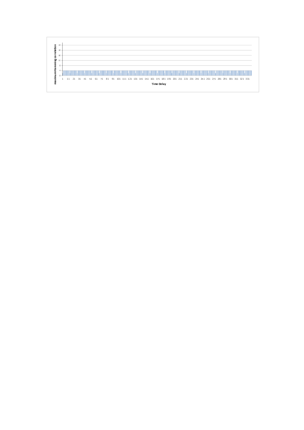
Then, the maximum Hamming correlation of 𝒮\mathcal{S} can be seen in Figure 1.

Refer to caption
Figure 1. The maximum Hamming correlations of 𝒮\mathcal{S} in Example 1

The maximum Hamming correlation of FHS set 𝒮\mathcal{S} in Example 1 is λ=4\lambda=4. Thus, it can be verified that SS is an optimal (338,91,4,3)(338,91,4;3) FHS set. In the similar way, 𝒳\mathcal{X} can be extended to an optimal FHS set with other parameters by choosing different n=q1⋯qrn=q_{1}\cdots q_{r}, and the extension factor nn should not co-prime to the length N=26N=26 of 𝒳\mathcal{X}.

5. Optimal FHS Sets of Length d​NdN

In this section, we present a new design for optimal FHS set with new parameters under the framework in Section 3. Our procedure of the extension construction is described as follows.

Construction 2.

Construction of optimal FHS sets of length d​NdN.

  1. Step 1:

    Select an optimal (N,v,λ,M)(N,v,\lambda;M) FHS set

    𝒳={𝐱i=(xi​(0),xi​(1),…,xi​(N−1)):0≤i≤M−1}.\mathcal{X}=\left\{{\bf x}_{i}=(x_{i}(0),x_{i}(1),\ldots,x_{i}(N-1)):0\leq i\leq M-1\right\}.

    The maximum number of appearance of frequency slot in 𝒳\mathcal{X} is m⁡(𝒳)m(\mathcal{X}).

  2. Step 2:

    Let q=paq=p^{a} for a prime pp and a positive integer aa. Let g′g^{\prime} be a primitive element of ∈ℤp∗\in\mathbb{Z}^{*}_{p}, so g=g′g=g^{\prime} or g=g′+pg=g^{\prime}+p is the primitive element of ℤq∗\mathbb{Z}^{*}_{q}, d=ord⁡(g)=(p−1)​p(a−1)d={\rm ord}(g)=(p-1)p^{(a-1)}. Generate a set

    ℰ={𝐞j=(g0+j,g1+j,⋯,gd−1+j):0≤j≤p−1}.\mathcal{E}=\{{\bf e}_{j}=(g^{0}+j,g^{1}+j,\cdots,g^{d-1}+j):0\leq j\leq p-1\}.
  3. Step 3:

    If m⁡(𝒳)≤pm(\mathcal{X})\leq p, ωi​(t2)\omega_{i}(t_{2}) be a function with ωi​(t2)=φfk​(i,t2)\omega_{i}(t_{2})=\varphi_{f_{k}}(i,t_{2}), where φfk\varphi_{f_{k}} is a injective function from Φk\Phi_{k} to Zl∗Z_{l}^{*} for every kk with 0≤k≤v0\leq k\leq v, 0≤i≤M−10\leq i\leq M-1, 0≤t2≤N−10\leq t_{2}\leq N-1, the set Φk\Phi_{k} is defined as Lemma 2.

  4. Step 4:

    We can construct the desired FHS set 𝒮={𝐬i:0≤i≤M−1}\mathcal{S}=\{{\bf s}^{i}:0\leq i\leq M-1\},

    𝐬i=I⁡[(𝐞ωi​(0),ai​(0)),(𝐞ωi​(1),ai​(1)),⋯,(𝐞ωi​(N−1),ai​(N−1))].{\bf s}^{i}=I[({\bf e}_{\omega_{i}(0)},a_{i}(0)),({\bf e}_{\omega_{i}(1)},a_{i}(1)),\cdots,({\bf e}_{\omega_{i}(N-1)},a_{i}(N-1))].
Lemma 6.

The set ℰ\mathcal{E} in Construction 2 has the following properties:
(i)(i) ℰ\mathcal{E} is a sequence set with pp sequences of length d=(p−1)​p(a−1)d=(p-1)p^{(a-1)} over ℤq\mathbb{Z}_{q};
(i​i)(ii) Ha​(ℰ)=0H_{a}(\mathcal{E})=0, Hc​(ℰ)=1H_{c}(\mathcal{E})=1;

Proof.

It is easily checked that the set ℰ\mathcal{E} in Construciton 2 is with pp sequences of length d=(p−1)​p(a−1)d=(p-1)p^{(a-1)} over ℤq\mathbb{Z}_{q}. For any 0≤t≤d−10\leq t\leq d-1, 0≤j1,j2≤p−10\leq j_{1},j_{2}\leq p-1, the Hamming correlation H𝐞j1​𝐞j2​(t)H_{{\bf e}_{j_{1}}{\bf e}_{j_{2}}}(t) between 𝐞j1{\bf e}_{j_{1}} and 𝐞j2{\bf e}_{j_{2}} is given by

H𝐞j1​𝐞j2​(t)\displaystyle H_{{\bf e}_{j_{1}}{\bf e}_{j_{2}}}(t) =\displaystyle= ∑i=0d−1h⁡(⟨gi+j1⟩q,⟨gi+t+j2⟩q).\displaystyle\sum\limits_{i=0}^{d-1}h\left(\langle g^{i}+{j_{1}}\rangle_{q},\langle g^{i+t}+{j_{2}}\rangle_{q}\right).

In order to compute H𝐞j1​𝐞j2​(t)H_{{\bf e}_{j_{1}}{\bf e}_{j_{2}}}(t), we divide the problem into two cases.

Case OPENi)i). j1=j2j_{1}=j_{2}.

In this case, we can easily obtain that

H𝐞j1​𝐞j1​(t)={d,t=0,0,o​t​h​e​r​w​i​s​e.\displaystyle H_{{\bf e}_{j_{1}}{\bf e}_{j_{1}}}(t)=\left\{{\begin{array}[]{*{20}{c}}d,&t=0,\\ 0,&otherwise.\\ \end{array}}\right.

Case OPENi​i)ii). j1≠j2j_{1}\neq j_{2}.

Since g=g′g=g^{\prime} or g=g′+p1g=g^{\prime}+p_{1} is the primitive element ∈ℤq1∗\in\mathbb{Z}^{*}_{q_{1}}, where g′g^{\prime} is a primitive element ∈ℤp1∗\in\mathbb{Z}^{*}_{p_{1}}. For any 0≤i≤d−10\leq i\leq d-1, 0≤t≤d−10\leq t\leq d-1, we have

⟨gi−gi+t⟩q={gρ,t≠p−1,σ​p,t=p−1,\displaystyle\langle g^{i}-g^{i+t}\rangle_{q}=\left\{{\begin{array}[]{*{20}{c}}g^{\rho},&t\neq p-1,\\ \sigma p,&t=p-1,\\ \end{array}}\right.

where 0≤ρ≤d−1,1≤σ<pa−10\leq\rho\leq{d-1},1\leq\sigma<p^{a-1}.

Thus, we have

H𝐞j1​𝐞j2​(t)\displaystyle H_{{\bf e}_{j_{1}}{\bf e}_{j_{2}}}(t) =\displaystyle= ∑i=0d−1h⁡(⟨gi+j1⟩q,⟨gi+t+j2⟩q)\displaystyle\sum\limits_{i=0}^{d-1}h\left(\langle g^{i}+{j_{1}}\rangle_{q},\langle g^{i+t}+{j_{2}}\rangle_{q}\right)
=\displaystyle= ∑i=0d−1h⁡(⟨gi−gi+t⟩q,⟨j2−j1⟩q).\displaystyle\sum\limits_{i=0}^{d-1}h\left(\langle g^{i}-g^{i+t}\rangle_{q},\langle j_{2}-j_{1}\rangle_{q}\right).

Without loss of generality, we can assume 0≤j1<j2≤p−10\leq j_{1}<j_{2}\leq p-1, so we have 0≤j2−j1≤p−10\leq j_{2}-j_{1}\leq p-1.

Hence, we can obtain from equation (7) that

H𝐞j1​𝐞j2​(t)​{1,t≠p−1,0,t=p−1.\displaystyle H_{{\bf e}_{j_{1}}{\bf e}_{j_{2}}}(t)\left\{{\begin{array}[]{*{20}{c}}1,&t\neq p-1,\\ 0,&t=p-1.\\ \end{array}}\right.

By summarizing the results of Case OPENi)i) and Case OPENi​i)ii), we have the nontrivial Hamming correlation of ℰ\mathcal{E} is

H𝐞j1​𝐞j2​(t)={0,j1=j2,t≠0,0,j1≠j2,t=p−1,1,j1≠j2,t≠p−1.\displaystyle H_{{\bf e}_{j_{1}}{\bf e}_{j_{2}}}(t)=\left\{{\begin{array}[]{*{20}{c}}0,&j_{1}=j_{2},t\neq 0,\\ 0,&j_{1}\neq j_{2},t=p-1,\\ 1,&j_{1}\neq j_{2},t\neq p-1.\\ \end{array}}\right.

∎

Theorem 2.

The FHS set 𝒮\mathcal{S} constructed by Construction 2 is an optimal (d​N,q​v,λ,M)(dN,qv,\lambda;M) FHS set over ℤq×ℱ\mathbb{Z}_{q}\times\mathcal{F} if ⌈(d​N​M−v)(q​N​M−1)​d​Nq​v⌉=⌈(N​M−v)(N​M−1)​Nv⌉\left\lceil\frac{(dNM-v)}{(qNM-1)}\frac{dN}{qv}\right\rceil=\left\lceil{\frac{{(NM-v)}}{{(NM-1)}}\frac{N}{v}}\right\rceil.

Proof.

It is easily checked that the extended FHS set 𝒮\mathcal{S} in Construciton 2 is a set with MM sequences of length d​NdN over ℤq×ℱ\mathbb{Z}_{q}\times\mathcal{F}, where d=(p−1)​p(a−1)d=(p-1)p^{(a-1)}.

From Lemma 3, the Hamming correlation of FHS set 𝒮\mathcal{S} is based on the correlation of set ℰ\mathcal{E}. Thus, from Lemma 5, we can obtain that Hm​(𝒮)=Hm​(𝒳)=λH_{m}(\mathcal{S})=H_{m}(\mathcal{X})=\lambda. Since the optimal FHS set 𝒳\mathcal{X} satisfies Peng-Fan bound [5], we have λ=⌈(N​M−v)(N​M−1)​Nv⌉\lambda=\left\lceil{\frac{{(NM-v)}}{{(NM-1)}}\frac{N}{v}}\right\rceil.

Then, we verify the optimality of the extended FHS set 𝒮\mathcal{S}. According to the Peng-Fan bound [5], the FHS set 𝒮\mathcal{S} with length d​NdN, the family size MM and the frequency slot set size q​vqv over ℤq×ℱ\mathbb{Z}_{q}\times\mathcal{F}, the optimal maximum Hamming correlation Hm′H^{\prime}_{m} of 𝒮\mathcal{S} is

Hm′≥⌈(d​N​M−v)(q​N​M−1)​d​Nq​v⌉.\displaystyle{H^{\prime}_{m}}\geq\left\lceil\frac{(dNM-v)}{(qNM-1)}\frac{dN}{qv}\right\rceil.

Thus, we have the FHS set 𝒮\mathcal{S} in Construction 2 is optimal if ⌈(d​N​M−v)(q​N​M−1)​d​Nq​v⌉=⌈(N​M−v)(N​M−1)​Nv⌉\left\lceil\frac{(dNM-v)}{(qNM-1)}\frac{dN}{qv}\right\rceil=\left\lceil{\frac{{(NM-v)}}{{(NM-1)}}\frac{N}{v}}\right\rceil.

∎

In particular, by generating the set ℰ\mathcal{E} in the finite field 𝔽q\mathbb{F}_{q}, it is possible to construct an extended FHS set of length d​NdN with different extension factor dd.

Corollary 3.

Let gg be a primitive element of 𝔽q\mathbb{F}_{q}, then we have d=ord⁡(g)=q−1d={\rm ord}(g)=q-1. Then, if m⁡(𝒳)≤qm(\mathcal{X})\leq q, the FHS set 𝒮\mathcal{S} constructed by Construction 2 is an optimal ((q−1)​N,q​v,λ,M)((q-1)N,qv,\lambda;M) FHS set over 𝔽q×ℱ\mathbb{F}_{q}\times\mathcal{F}.

Remark 2.

By means of our method, Chung’s Construction B in [25] is a special case of Corollary 3 for gcd⁡(q−1,N)=1\gcd(q-1,N)=1 and ωi​(t2)=∑α=0i−1∑t=0N−1h⁡(xα​(t),xi​(t2))+∑β=0t2−1h⁡(xi​(β),xi​(t2))−1\omega_{i}(t_{2})=\sum^{i-1}_{\alpha=0}\sum^{N-1}_{t=0}h(x_{\alpha}(t),x_{i}(t_{2}))+\sum^{t_{2}-1}_{\beta=0}h(x_{i}(\beta),x_{i}(t_{2}))-1 for any 0≤i≤M−1,0≤t2≤N−10\leq i\leq M-1,0\leq t_{2}\leq N-1.

Therefore, it is possible to extend the length of 𝒮\mathcal{S} in Construction 2 by the extension factor n=q1⋯qrn=q_{1}\cdots q_{r}, if m⁡(𝒳)≤p1−1m(\mathcal{X})\leq p_{1}-1, where qi=piai,1≤i≤rq_{i}=p^{a_{i}}_{i},1\leq i\leq r, p1,…,prp_{1},\ldots,p_{r} are primes with p1<…<prp_{1}<\ldots<p_{r}. In this way, Construction 2 can be applied recursively infinitely many times.

Corollary 4.

For positive integers rr and a,a1,…,ara,a_{1},\ldots,a_{r}, let n=q1⋯qrn=q_{1}\cdots q_{r}, where q=paq=p^{a}, qi=piai,1≤i≤rq_{i}=p^{a_{i}}_{i},1\leq i\leq r, p,p1,…,prp,p_{1},\ldots,p_{r} are primes with p1<…<prp_{1}<\ldots<p_{r}. If m⁡(𝒳)≤min⁡{p1−1,p}m(\mathcal{X})\leq\min\{p_{1}-1,p\}, there exists an optimal (n​d​N,n​q​v,λ,M)(ndN,nqv,\lambda;M) FHS set over ℤqr×⋯×ℤq1×ℤq×ℱ\mathbb{Z}_{q_{r}}\times\cdots\times\mathbb{Z}_{q_{1}}\times\mathbb{Z}_{q}\times\mathcal{F}, d=(p−1)​p(a−1)d=(p-1)p^{(a-1)}.

Corollary 5.

Let gg be a primitive element of 𝔽q\mathbb{F}_{q}, then the extension factor is d=ordd={\rm ord}(g)=q−1(g)=q-1. Thus, if m⁡(𝒳)≤min⁡{p1−1,q}m(\mathcal{X})\leq\min\{p_{1}-1,q\}, the FHS set 𝒮\mathcal{S} constructed by Construction 2 is an optimal (n⁡(q−1)​N,n​q​v,λ,M)(n(q-1)N,nqv,\lambda;M) FHS set over ℤqr×⋯×ℤq1×𝔽q×ℱ\mathbb{Z}_{q_{r}}\times\cdots\times\mathbb{Z}_{q_{1}}\times\mathbb{F}_{q}\times\mathcal{F}.

Some new optimal FHS sets obtained by recursively applying Construction 2 are listed in Table 2. Since Construction 2 can be applied to any existing optimal FHSs or FHS sets, it is expected that there exist some more classes of optimal FHS sets which can be obtained from our construction, but are not listed there.

Table 2. The parameters of some new optimal FHS Sets obtained by combining Construction 1 and Construction 2.
New FHS sets Constraints References
(n​d​(αm−1),n​q​αl,αm−l,αl)\left(nd(\alpha^{m}-1),nq\alpha^{l},\alpha^{m-l};\alpha^{l}\right)
1≤l≤m1\leq l\leq m,
d=(p−1)​pa−1d=(p-1)p^{a-1}, αm<min⁡{p,lpf⁡(n)−1}\alpha^{m}<\min\{p,{\rm lpf}(n)-1\}.
or d=pa−1d=p^{a}-1, αm<min⁡{q,lpf⁡(n)−1}\alpha^{m}<\min\{q,{\rm lpf}(n)-1\}.
[4]
(n​d​α2,n​q​α,α,α)\left(nd\alpha^{2},nq\alpha,\alpha;\alpha\right)
d=(p−1)​pa−1d=(p-1)p^{a-1}, α2≤min⁡{p,lpf⁡(n)−1}\alpha^{2}\leq\min\{p,{\rm lpf}(n)-1\}.
or d=pa−1d=p^{a}-1, α2≤min⁡{q,lpf⁡(n)−1}\alpha^{2}\leq\min\{q,{\rm lpf}(n)-1\}.
[6, 22]
(n​d​α,n​q​(e+1),g,e)\left(nd\alpha,nq(e+1),g;e\right)
α=e​g+1,2≤g<e\alpha=eg+1,2\leq g<e,
d=(p−1)​pa−1d=(p-1)p^{a-1}, α<min⁡{p,lpf⁡(n)−1}\alpha<\min\{p,{\rm lpf}(n)-1\}.
or d=pa−1d=p^{a}-1, α<min⁡{q,lpf⁡(n)−1}\alpha<\min\{q,{\rm lpf}(n)-1\}.
[8]
(n​d​(r−1),n​q​(e+1),g,e)\left(nd(r-1),nq(e+1),g;e\right)
r=e​g+1,r−1≤e⁡(e+1)r=eg+1,r-1\leq e(e+1),
d=(p−1)​pa−1d=(p-1)p^{a-1}, r<min⁡{p,lpf⁡(n)−1}r<\min\{p,{\rm lpf}(n)-1\}.
or d=pa−1d=p^{a}-1, r<min⁡{q,lpf⁡(n)−1}r<\min\{q,{\rm lpf}(n)-1\}.
[11, 14]
(n​d​rm−1,n​q​rl,rm−l,rl)\left(ndr^{m}-1,nqr^{l},r^{m-l};r^{l}\right)
1≤l≤m1\leq l\leq m,
d=(p−1)​pa−1d=(p-1)p^{a-1}, rm<min⁡{p,lpf⁡(n)−1}r^{m}<\min\{p,{\rm lpf}(n)-1\}.
or d=pa−1d=p^{a}-1, rm<min⁡{q,lpf⁡(n)−1}r^{m}<\min\{q,{\rm lpf}(n)-1\}.
[17]
(n​d​rm−1h,n​q​rl,rm−l−1h,h)\left(\frac{ndr^{m}-1}{h},nqr^{l},\frac{r^{m-l}-1}{h};h\right)
gcd⁡(h,m)=1\gcd(h,m)=1, h|r−1h|r-1, 1≤l≤m1\leq l\leq m,
d=(p−1)​pa−1d=(p-1)p^{a-1}, rm−l<min⁡{p,lpf⁡(n)−1}r^{m-l}<\min\{p,{\rm lpf}(n)-1\}.
or d=pa−1d=p^{a}-1, rm−l<min⁡{q,lpf⁡(n)−1}r^{m-l}<\min\{q,{\rm lpf}(n)-1\}.
[17]

In Table 2, lpf⁡(n){\rm lpf}(n) denotes the least prime factor of nn, q=paq=p^{a} for a prime pp, rr is a prime power for a prime α\alpha.

Construction 2 in the case of M=1M=1 leads to the construction of a new single FHS. Based on Construction 2, it is possible to obtain new optimal FHSs with respect to the Lempel-Greenberger bound.

Corollary 6.

Assume that there exists an optimal (N,v,λ)(N,v,\lambda)-FHS 𝐬{\bf s} with respect to the Lempel-Greenberger bound, defined over ℱ\mathcal{F}. For positive integers rr and a,a1,…,ara,a_{1},\ldots,a_{r}, n=q1⋯qrn=q_{1}\cdots q_{r}, where q=pa,qi=piai,1≤i≤rq=p^{a},q_{i}=p^{a_{i}}_{i},1\leq i\leq r, p,p1,…,prp,p_{1},\ldots,p_{r} are primes with p1<…<prp_{1}<\ldots<p_{r}. Then, there exists an optimal (n​d​N,n​q​v,λ)(ndN,nqv,\lambda)-FHS over ℤqr×⋯×ℤq1×ℤq×ℱ\mathbb{Z}_{q_{r}}\times\cdots\times\mathbb{Z}_{q_{1}}\times\mathbb{Z}_{q}\times\mathcal{F}, if m⁡(𝒳)≤min⁡{p1−1,q}m(\mathcal{X})\leq\min\{p_{1}-1,q\}, d=pa−1d=p^{a}-1, or m⁡(𝒳)≤min⁡{p1−1,p}m(\mathcal{X})\leq\min\{p_{1}-1,p\}, d=(p−1)​p(a−1)d=(p-1)p^{(a-1)}.

Example 2.

We select an optimal (8,3,3,3)(8,3,3;3) FHS set 𝒴={𝐲0,𝐲1,𝐲2}\mathcal{Y}=\{{\bf y}_{0},{\bf y}_{1},{\bf y}_{2}\} over ℤ3\mathbb{Z}_{3}, such that

𝐲0={0,2,2,1,0,1,1,2},\displaystyle{\bf y}_{0}=\{0,2,2,1,0,1,1,2\},
𝐲1={1,0,0,2,1,2,2,0},\displaystyle{\bf y}_{1}=\{1,0,0,2,1,2,2,0\},
𝐲2={2,1,1,0,2,0,0,1}.\displaystyle{\bf y}_{2}=\{2,1,1,0,2,0,0,1\}.

So, we have m⁡(𝒴)=8m(\mathcal{Y})=8.

Select a=2a=2, and q=p2=121q=p^{2}=121, p=11>m⁡(𝒴)=8p=11>m(\mathcal{Y})=8. Choose g=2g=2 is the primitive element of ℤp∗\mathbb{Z}^{*}_{p} and ℤq∗\mathbb{Z}^{*}_{q}.

Generate a sequence set ℰ={𝐞j=(g0+j,g1+j,⋯,gd−1+j):0≤j≤10}\mathcal{E}=\{{\bf e}_{j}=(g^{0}+j,g^{1}+j,\cdots,g^{d-1}+j):0\leq j\leq 10\}, which can be written as

𝐞0={1,2,4,8,16,32,64,7,14,28,56,112,103,85,49,98,75⋯},\displaystyle{\bf e}_{0}=\{1,2,4,8,16,32,64,7,14,28,56,112,103,85,49,98,75\cdots\},
𝐞1={2,3,5,9,17,33,65,8,15,29,57,113,104,86,50,99,76⋯},\displaystyle{\bf e}_{1}=\{2,3,5,9,17,33,65,8,15,29,57,113,104,86,50,99,76\cdots\},
𝐞10={11,12,14,18,26,42,74,17,24,38,66,1,113,95,59,108,85⋯}.\displaystyle{\bf e}_{10}=\{11,12,14,18,26,42,74,17,24,38,66,1,113,95,59,108,85\cdots\}.

For any 0≤i≤20\leq i\leq 2, 0≤t2≤70\leq t_{2}\leq 7, a special expression of ω={ω0,ω1,ω2}\omega=\{\omega_{0},\omega_{1},\omega_{2}\} can be given by

ω0={0,0,1,0,1,1,2,2},\displaystyle\omega_{0}=\{0,0,1,0,1,1,2,2\},
ω1={3,2,3,3,4,4,5,4},\displaystyle\omega_{1}=\{3,2,3,3,4,4,5,4\},
ω2={6,5,6,5,7,6,7,7}.\displaystyle\omega_{2}=\{6,5,6,5,7,6,7,7\}.

Then we can construct the FHS set 𝒮={𝐬0,𝐬1,𝐬2}\mathcal{S}=\{{\bf s}_{0},{\bf s}_{1},{\bf s}_{2}\} by the Construction 2.

𝐬0\displaystyle{\bf s}_{0} =\displaystyle= {(1,0),(1,2),(2,2),(1,1),(2,0),(2,1),(3,1),(3,2),(2,0),(2,2),(3,2),(2,1),…,\displaystyle\{(1,0),(1,2),(2,2),(1,1),(2,0),(2,1),(3,1),(3,2),(2,0),(2,2),(3,2),(2,1),\ldots,
(92,1),(93,1),(93,2),(61,0),(61,2),(62,2),(61,1),(62,0),(62,1),(63,1),(63,2)},\displaystyle(92,1),(93,1),(93,2),(61,0),(61,2),(62,2),(61,1),(62,0),(62,1),(63,1),(63,2)\},
𝐬1\displaystyle{\bf s}_{1} =\displaystyle= {(4,1),(3,0),(4,0),(4,2),(5,1),(5,2),(6,2),(5,0),(5,1),(4,0),(5,0),(5,2),…,\displaystyle\{(4,1),(3,0),(4,0),(4,2),(5,1),(5,2),(6,2),(5,0),(5,1),(4,0),(5,0),(5,2),\ldots,
(95,2),(96,2),(95,0),(64,1),(63,0),(64,0),(64,2),(65,1),(65,2),(66,2),(65,0)},\displaystyle(95,2),(96,2),(95,0),(64,1),(63,0),(64,0),(64,2),(65,1),(65,2),(66,2),(65,0)\},
𝐬2\displaystyle{\bf s}_{2} =\displaystyle= {(7,2),(6,1),(7,1),(6,0),(8,2),(7,0),(8,0),(8,1),(8,2),(7,1),(8,1),(7,0),…,\displaystyle\{(7,2),(6,1),(7,1),(6,0),(8,2),(7,0),(8,0),(8,1),(8,2),(7,1),(8,1),(7,0),\ldots,
(97,0),(98,0),(98,1),(67,2),(66,1),(67,1),(66,0),(68,2),(67,0),(68,0),(68,1)}.\displaystyle(97,0),(98,0),(98,1),(67,2),(66,1),(67,1),(66,0),(68,2),(67,0),(68,0),(68,1)\}.

The FHS 𝐬0{\bf s}_{0} over ℤ121×ℤ3\mathbb{Z}_{121}\times\mathbb{Z}_{3} can be obtained from the 110×8110\times 8 array in (8)(8), that is

((1,0)(1,2)(2,2)(1,1)(2,0)(2,1)(3,1)(3,2)(2,0)(2,2)(3,2)(2,1)(3,0)(3,1)(4,1)(4,2)(4,0)(4,2)(5,2)(4,1)(5,0)(5,1)(6,1)(6,2)⋮⋮⋮⋮⋮⋮⋮⋮(91,0)(91,2)(92,2)(91,1)(92,0)(92,1)(93,1)(93,2)(61,0)(61,2)(62,2)(61,1)(62,0)(62,1)(63,1)(63,2)).\displaystyle\left(\small{\begin{array}[]{*{10}{c}}(1,0)&(1,2)&(2,2)&(1,1)&(2,0)&(2,1)&(3,1)&(3,2)\\ (2,0)&(2,2)&(3,2)&(2,1)&(3,0)&(3,1)&(4,1)&(4,2)\\ (4,0)&(4,2)&(5,2)&(4,1)&(5,0)&(5,1)&(6,1)&(6,2)\\ \vdots&\vdots&\vdots&\vdots&\vdots&\vdots&\vdots&\vdots\\ (91,0)&(91,2)&(92,2)&(91,1)&(92,0)&(92,1)&(93,1)&(93,2)\\ (61,0)&(61,2)&(62,2)&(61,1)&(62,0)&(62,1)&(63,1)&(63,2)\end{array}}\normalsize\right).

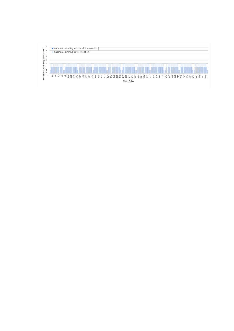
Then, the maximum Hamming correlation of 𝒮\mathcal{S} can be seen in Figure 2.

Refer to caption
Figure 2. The maximum Hamming correlations of 𝒮\mathcal{S} in Example 2

The maximum Hamming correlation in Example 2 is λ=3\lambda=3. Thus, It can be verified that 𝒮\mathcal{S} is an optimal (880,363,3,3)(880,363,3;3) FHS set. In a similar way, original FHS set 𝒴\mathcal{Y} can be extended to an optimal FHS set with new parameters, and the extension factor dd should not co-prime to the length N=8N=8 of 𝒴\mathcal{Y}.

6. Conclusions

In this paper, we present a framework of constructing optimal FHS sets based on the designated direct product, which increase the length and alphabet size of the original FHS set, but preserve its maximum Hamming correlation. The framework generalize the previous extension constructions of optimal FHS sets. Under the framework, we obtain infinitely many new optimal FHS sets by combining a family of sequences that are newly constructed in this paper with some known optimal FHS sets. Compared with the previous extension methods in [25,26], our construction remove the constraint requiring that the expansion factor is co-prime with the length of original FHSs and get new parameters, as shown in Table 1. As a result, we have a great flexibility of choosing parameters of FHS sets for a given frequency hopping spread spectrum system.

References

  • [1] P. Fan and M. Darnell, Sequence design for communications applications. London, U.K.: Wiley, 1996.
  • [2] S. W. Golomb, G. Gong, Signal design for good correlation: for wireless communication, cryptography and radar. U.K.: Cambridage Univ. Press, 2005.
  • [3] M. K. Simon, J. K. Omura, R. A. Scholtz, and B. K. Levitt, Spread spectrum communications handbook. New York, NY, USA: McGraw-Hill, 1994.
  • [4] A. Lempel, H. Greenberger, “Families sequence with optimal Hamming correlation properties,” IEEE Trans. Inf. Theory, vol.IT-20, pp. 90-94, Jan. 1974.
  • [5] D. Y. Peng, P. Z. Fan, “Lower bounds on the Hamming auto- and cross correlations of frequency hopping sequences,” IEEE Trans. Inf. Theory, vol.50, no.9, pp.2149-2154, Sep. 2004.
  • [6] P. V. Kumar, “Frequency-hopping code sequence designs having large linear span,” IEEE Trans. Inf. Theory, vol. 34, no. 1, pp. 146-151, Jan. 1988.
  • [7] P. Udaya and M. U. Siddiqi, “Optimal large linear complexity frequency hopping patterns derived from polynomial residue class rings,” IEEE Trans. Inf. Theory, vol. 44, no. 4, pp. 1492-1503, Jul. 1998.
  • [8] W. Chu and C. J. Colbourn, “Optimal frequency-hopping sequences via cyclotomy,” IEEE Trans. Inf. Theory, vol. 51, no. 3, pp. 1139-1141, Mar. 2005.
  • [9] Z. Cao, G. Ge, and Y. Miao, “Combinatorial characterizations of onecoincidence frequency-hopping sequences,” Des. Codes Cryptograph., vol. 41, no. 2, pp. 177-184, Nov. 2006.
  • [10] G. Ge, R. Fuji-Hara, and Y. Miao, “Further combinatorial constructions for optimal frequency hopping sequences,” J. Combinat. Theory, Ser. A, vol. 113, no. 8, pp. 1699-1718, 2006.
  • [11] C. Ding and J. Yin, “Sets of optimal frequency-hopping sequences,” IEEE Trans. Inf. Theory, vol. 54, no. 8, pp. 3741-3745, Aug. 2008.
  • [12] G. Ge, Y. Miao, and Z. Yao, “Optimal frequency hopping sequences: Auto- and cross-correlation properties,” IEEE Trans. Inf. Theory, vol. 55, no. 2, pp. 867-879, Feb. 2009.
  • [13] C. Ding, R. Fuji-Hara, Y. Fujiwara, M. Jimbo, and M. Mishima, “Sets of frequency hopping sequences: Bounds and optimal constructions,” IEEE Trans. Inf. Theory, vol. 55, no. 7, pp. 3297-3304, Jul. 2009.
  • [14] Y.K. Han, K. Yang, “On the Sidel¡¯nikov sequences as frequency-hopping sequences,” IEEE Trans. Inf. Theory, vol. 55, no. 9, pp. 4279-4285, Sep. 2009.
  • [15] J.-H. Chung and K. Yang, “Optimal frequency-hopping sequences with new parameters,” IEEE Trans. Inf. Theory, vol. 56, no. 4, pp. 1685-1693, Apr. 2010.
  • [16] J.-H. Chung and K. Yang, “k-fold cyclotomy and its application to frequency-hopping sequences,” IEEE Trans. Inf. Theory, vol. 57, no. 4, pp. 2306-2317, Apr. 2011.
  • [17] Z. Zhou, X. Tang, D. Peng, and U. Parampalli, “New constructions for optimal sets of frequency-hopping sequences,” IEEE Trans. Inf. Theory, vol. 57, no. 6, pp. 3831-3840, Jun. 2011.
  • [18] Y. Yang, X. Tang, U. Parampalli, and D. Peng, “New bound on frequency hopping sequence sets and its optimal constructions,” IEEE Trans. Inf. Theory, vol. 57, no. 11, pp. 7605-7613, Nov. 2011.
  • [19] Z. Zhou, X. Tang, X. Niu, and U. Parampalli, “New classes of frequencyhopping sequences with optimal partial correlation,” IEEE Trans. Inf. Theory, vol. 58, no. 1, pp. 453-458, Jan. 2012.
  • [20] J.-H. Chung and K. Yang, “A new class of balanced near-perfect nonlinear mappings and its application to sequence design,” IEEE Trans. Inf. Theory, vol. 59, no. 2, pp. 1090-1097, Feb. 2013.
  • [21] X. Zeng, H. Cai, X. Tang, and Y. Yang, “Optimal frequency-hopping sequences of odd length,” IEEE Trans. Inf. Theory, vol. 59, no. 5, pp. 3237-3248, May 2013.
  • [22] X.D. Xu, X.W. Cao, G.K. Xu, “Optimal frequency-Hopping sequence sets based on cyclotomy,” Int. J. Found. Comput. Sci., vol. 27, no. 4, pp.1080-1086, Jun. 2016.
  • [23] J.H. Chung, Y. K. Han, and K. Yang, “New classes of optimal frequency-hopping sequences by interleaving techniques,” IEEE Trans. Inf. Theory, vol. 55, no. 12, pp. 5783-5791, Dec. 2009.
  • [24] X. Zeng, H. Cai, X. Tang, and Y. Yang, “A class of optimal frequency hopping sequences with new parameters,”IEEE Trans. Inf. Theory, vol. 58, no. 7, pp. 4899-4907, Jul. 2012.
  • [25] J. H. Chung, G. Gong, K. Yang, “New families of optimal frequency-hopping sequences of composite lengths,” IEEE Trans. Inf. Theory, vol. 60, no.6, pp.3688-3697, Jun. 2014.
  • [26] X.D. Xu, X.W. Cao, G.K. Xu, “Recursive construction of optimal frequency-hopping sequence sets,” IET Communications, vol. 10, no. 9, pp.1080-1086, Jun. 2016.