Exact holographic tensor networks for the Motzkin spin chain

The Motzkin Hamiltonian can be defined by first identifying each local spin-$z$ basis state $\{\ket{1},\ket{0},\ket{-1}\}$ with a line segment $\{\diagup,\text{{---}},\diagdown\}$, respectively. This allows us to represent states as a superposition of walks. The Hamiltonian, defined on a spin-chain with $2n$ sites reads:

where $\Pi_{j}$ acts on the pair of spins $j,j+1$ and

where $\Phi,\Psi,\Theta$ are the following states on pairs of neighboring spins

To have periodic boundary conditions, the Hamiltonian in Eq. (18) can be simply modified to include a $\Pi_{2n}$ term while omitting the boundary terms $\Pi_{\text{boundary}}$.

To re-purpose the binary-height network for the spin-1/2 Fredkin model, we define an operator $P\in\text{Hom}(\mathbb{C}^{3},\mathbb{C}^{2})$ that projects out the $0$ component of each spin and maps $1\mapsto\tfrac{1}{2}$ and $-1\mapsto-\tfrac{1}{2}$. It is given by

$\displaystyle\tikzpicture\scope\node{$\displaystyle P=\ket{\tfrac{1}{2}}\bra{1}+\ket{-\tfrac{1}{2}}\bra{-1}=$};\scope[xshift=2.4cm]\node{\includegraphics[width=10.34958pt]{Pop}};$

(22)

where the indices $k_{1}$ and $k_{2}$ are associated with the spin-1 and spin-$\tfrac{1}{2}$ degrees of freedom, respectively. Appending $P^{\otimes 2n}$ to the bottom of the binary-height tensor network yields a tensor network for the Fredkin model:

(23)

We note that Salberger and Korepin previously presented an MPS description of the Fredkin state using the height representation of Dyck walks [24]. However, the elementary building blocks of such networks have growing bond-dimension and lack the local structure of the networks we achieve here.

In this appendix we provide an alternative derivation of an exact hierarchical tensor network representation of the ground state of the spin-$1$ Motzkin spin chain. Here, in order to better connect with established tensor network methodology [33], we formulate the solution in terms of U(1) invariant tensors instead of the ‘flux’ preserving tiles discussed in the main text; however both approaches are ultimately equivalent. The derivation presented here is based on the dual notions of $\delta$-symmetric tensors, a restricted subclass of U(1) tensors, and boundary-locked networks. We first define these concepts before proceeding to demonstrate how they can be used to construct a network for the Motzkin spin chain.

Let us recall the basics of U(1)-symmetric networks, as detailed in Ref.[33]. A tensor network with U(1) symmetry is represented by an oriented graph, where each index has an associated direction (depicted with an arrow), such that the indices connected to a tensor can be regarded as either incoming or outgoing with respect to that tensor. Each index $i\in\{1,2,\ldots,d\}$ in the network is assigned a set of quantum numbers $\vec{n}^{(i)}=[n^{(i)}_{1},n^{(i)}_{2},\dots,n^{(i)}_{d}]$ with charges $n\in\mathbb{Z}$ associated to the $z$-component of the spin at that value of the index. We say that a tensor is U(1) symmetric if it is left invariant under transformation with a unitary representation of U(1) acting on each index (where outgoing indices should be transformed by the dual representation of U(1) with respect to incoming indices). It is known that U(1)-symmetric tensors are those that conserve particle number, such that a tensor component has zero weight unless the sum of the outgoing charges matches the sum of the incoming charges. For the purposes of constructing a solution to the Motzkin model, it is useful to restrict to a sub-class of symmetric tensors that we call $\delta$-symmetric tensors, which we define as U(1)-symmetric tensors where every (structurally non-zero) element is equal to unity. In other words, these are U(1)-symmetric tensors with component equal to unity if the total incoming charge $n_{\textrm{in}}$ matches the total outgoing charge $n_{\textrm{out}}$ and zero otherwise, which can be understood as a tensor version of the Kronecker-delta function.

The concept of a boundary-locked tensor network is now defined. Given a lattice $\mathcal{L}$ of spin-1 sites, let $T$ be the tensor network built from U(1)-symmetric tensors, representing a $S_{z}=0$ quantum state $\ket{\psi}\in\mathcal{L}$, and let $\ket{\phi}$ be a U(1)-invariant product state ($S_{z}=0$) on $\mathcal{L}$. We say that network $T$ if boundary-locked if, by constraint of the U(1) symmetry, there is a single unique configuration of the internal indices in $T$ that can give a non-zero contribution to the scalar product $\braket{\phi|\psi}$ for any input product state $\ket{\phi}$ with $S_{z}=0$. In other words, a network is boundary locked if, by fixing the boundary indices in a configuration compatible the $S_{z}=0$ symmetry of the network, the internal indices are then ‘locked’ in a unique configuration by the constraint that the total incoming U(1) charges must match the total outgoing charge in all tensors. It follows that a necessary (but not sufficient) constraint for a network to be boundary locked is that the irrep of charge $n$ on any tensor index is at most 1-fold degenerate (which allows us to specify the value that an index takes by the charge $n$ that it carries).

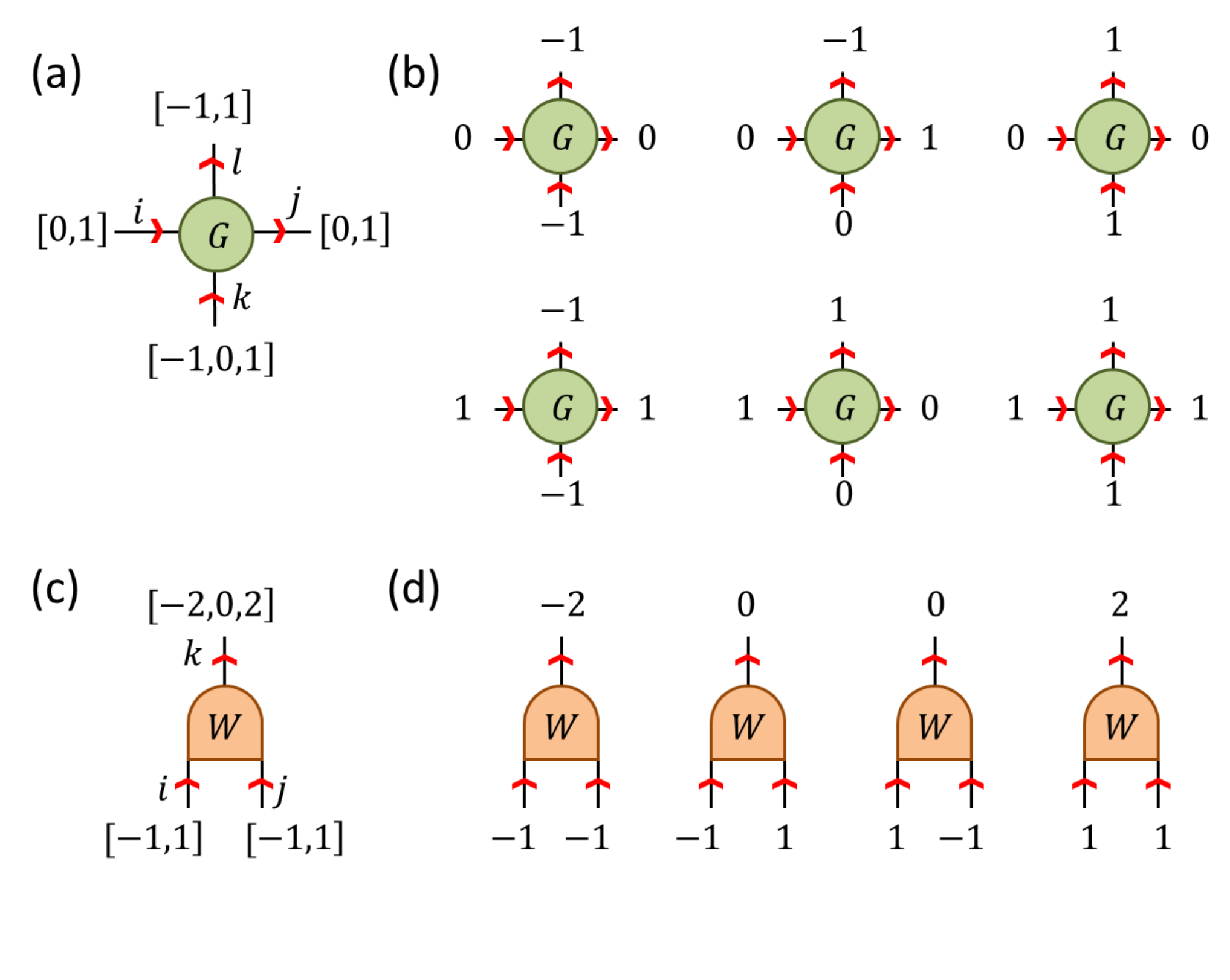
Given that the notions of $\delta$-symmetric tensors and boundary-locked networks have been established, we are now able to construct the exact hierarchical network for the ground state of the Motzkin chain. We begin by focusing on a simpler task: given a finite chain of spin-$1$ sites $\mathcal{L}$ we describe how to construct a network representing the equal weight superposition U(1) states in the $S_{z}=0$ spin symmetry sector (or equivalently, the superposition of all walks that start and end at zero height). This solution can later be refined to exclude the paths that take negative height values at any point, as described in the main text, such that the ground state of the original Motzkin spin chain is recovered. Let us consider a U(1)-invariant state $\ket{\psi}\in\mathcal{L}$ with $S_{z}=0$; if $\ket{\psi}$ is described by a boundary locked network built from $\delta$-symmetric tensors it automatically follows that $\ket{\psi}$ must be the desired equal-weight superposition of all states in the $S_{z}=0$ sector. This is true since the scalar product of $\ket{\psi}$ with any product state of the $S_{z}=0$ spin sector must evaluate to unity, as only a single configuration of indices can contribute and all configurations have a total weight equal to unity, while the scalar product with any state outside of the $S_{z}=0$ is trivially zero.

The remaining goal is thus is to build a boundary-locked network $T$of $\delta$-invariant tensors that constitutes a proper holographic realization: given a lattice $\mathcal{L}$ of $N$ sites, we want the network $T$ to be organized into $O(\log N)$ self-similar layers, each with some finite bond dimension that is independent of the system size $N$. Here we follow a similar construction as used in the MERA, and build the network from a sequence of coarse graining (CG) transformations, each of which is comprised of a disentangling step followed by a blocking step that reduces the number of lattice sites by a factor of $2$. However, instead of using disentanglers with finite local support, which prove inadequate for the exact construction, we instead represent the disentangling operation as an MPO. We build this MPO from copies of a four index $\delta$-invariant tensor $G^{ik}_{jl}$ as depicted in Fig. 6(a-b). The virtual bond dimension of the MPO is set at $d=2$, with U(1) charges on these indices $\vec{n}^{(i)}=\vec{n}^{(j)}=[0,1]$. The incoming indices $k$ must match the spin-$1$ sites in $\mathcal{L}$, i.e. such that $\vec{n}^{(k)}=[-1,0,1]$, while the output indices $l$ are set at $d=2$ with U(1) charges $\vec{n}^{(l)}=[-1,1]$. Thus the action of this MPO is to map states on the $N$-site lattice $\mathcal{L}$, which has local dimension $d=3$, to states on an $N$-site lattice $\mathcal{L}^{\prime}$ of local dimension $d=2$. If we assume $N$ to be even and that the virtual indices of the edge MPO tensors are fixed in the $\ket{0}$ state, then it can be seen that any $S_{z}=0$ product state on $\mathcal{L}$ is mapped to a unique product state on $\mathcal{L}^{\prime}$, see Fig. 7 for example, consistent with the desire for a boundary-locked network. This follows as, once the input indices $i$ and $k$ have been set on a $G$ tensor, there is only a single choice of the output indices $j$ and $l$ that satisfies U(1) charge conservation. The blocking step of the CG transformation is now realized using a 3-index $\delta$-symmetric tensor $W^{ij}_{k}$, whose input indices carry U(1) charges $\vec{n}^{(i)}=\vec{n}^{(j)}=[-1,1]$ and whose output index carries $\vec{n}^{(k)}=[-2,0,2]$, see also Fig. 6(c-d). This blocking step is again consistent with realizing a boundary locked network, and clearly has non-zero overlap with any state on $\mathcal{L}^{\prime}$.

One may then repeat this coarse graining transformation, consisting of disentangling with the MPO formed from $G$ tensors and then blocking with the $W$. Notice that the magnitude of U(1) individual charges carried on the indices of the $G$ and $W$ tensors doubles with each coarse graining step, but the content of these tensors otherwise remains unchanged. The output index on the final isometry, after taking $\log_{2}(N)$ coarse graining steps where $N$ is assumed to be a power of 2, is fixed in the $n=0$ state to ensure that the network is in the total spin $S_{z}=0$ sector, see Fig. 8. Thus our goal is completed: we have an $S_{z}=0$ holographic network that (i) is constructed entirely from $\delta$-symmetric tensors and (ii) is boundary-locked, which implies that it represents an equal weighted superposition of all states in the total spin $S_{z}=0$ sector.

In comparing the network derived in this appendix, Fig. 8(a), to that derived in the main text, Fig. 4, one sees that they both have an equivalent structure, with the $G$ and $W$ tensors derived in this appendix substituting for the $B$ and $T$ tensors in Fig. 4. However, upon expressing the $G$ and $W$ tensors in the ‘tiling’ representation used in the main text, see Fig. 9(a-b), it is seen that they correspond to a different set of tiles than do the $B$ tensors, Fig. 2, and the $T$ tensors, Fig. 4. Nevertheless, a component-wise analysis of all permissible tilings reveals that the product of two $G$ and a $W$ tensor is identical to the product of two $B$ and a $T$ tensor, as depicted in Fig. 9(c). Thus one indeed concludes that the network constructed in this appendix is ultimately equivalent to that of the main text.

Here we prove that the height renormalization tensor network defined in Fig. 4 represents the periodic Motzkin ground state. We do this by showing its equivalence to the generalized binary-height tensor network defined in Fig. 2(b).

In order to represent the state $\ket{\Psi_{k}}$, the boundary vectors $\ket{\vec{b}_{\text{L}}}$ and $\ket{\vec{b}_{\text{R}}}$ (see Eq. (6)) are chosen to encode integers $p$ and $q$ such that $q-p=k$ and $\text{min}(p,q)\geq n$. We choose

We use a rectangular binary-height tensor network with $m=2^{\lfloor\log_{2}2n\rfloor+1}$ many layers. This choice guarantees that $b_{m\text{L}}=b_{m\text{R}}=1$. See Fig. 10(a) for an example on 8 spins.

As usual, the upwards pointing indices on the $m^{\text{th}}$ layer have been contracted with the state $\ket{0}$. In fact, all such indices must take the value 0 regardless of this boundary condition. To see this, suppose some of these indices took a value of 1 or -1, and let $\mu$ be the leftmost column with a non-zero value at the top.

Then,

• •

  If the top index of $\mu$ takes value $-1$, the only valid tiling for $\mu$ is to use tile $A_{6}$ for all square cells. Then, the height encoded at the left boundary of $\mu$ is zero. However, from Eq. (25), $p>2n\geq\mu$, and since it takes at least $y$ many columns to drop in height by $y$, there are no valid tilings of the lattice to the left of $\mu$.

• •

  If the top index of $\mu$ takes value $1$, the only valid tiling for $\mu$ is to use tile $A_{2}$ for all square cells. Then, the height encoded at the right boundary of $\mu$ is zero. However, from Eq. (25), $q>2n\geq 2n-\mu$, and since it takes at least $y$ many columns to climb in height by $y$, there are no valid tilings of the lattice to the right of $\mu$.

Because non-zero values at the top indices of the network yield invalid tilings, contractions of the network must evaluate to zero in such cases.

Therefore, there is some flexibility in choosing the upper boundary condition, i.e., we are free to replace the contraction with $\ket{0}^{\otimes 2n}$ with any other tensor that has equal support over this state. In particular, we can use a binary tree of triangle $T$ tensors, as shown in Fig. 10(b). Tiling the entire pyramid with $D_{5}$ tiles shows that it has support over the $\ket{0}^{\otimes 2n}$ subspace.

Next, we require following lemma:

Using this, we can pull a horizontal layer of triangular tensors in Fig. 10(b) downwards through the tensor network. At each step, two $B$ tensors are merged into one. Pulling down each triangular tensor is analogous to closing a zipper. The end result is shown in Fig. 10(c).

The final step to prove equivalence with the height renormalization tensor network from Fig. 4(a) is to note that the top $B$ tensor from Fig. 10(c) can be removed, since

(28)

Removing the top $B$ tensor modifies the left and right boundary heights so that now $\text{max}(p,q)=2n$ and $\text{min}(p,q)=2n-|k|$.

Here we show that the height renormalization tensor network shown in Fig. 5 is a valid representation of the Motzkin model. Our proof will follow a similar trajectory to the case with periodic boundary conditions.

We begin with the step-pyramid of $B$ tensors from Fig. 2. We will embed the width $2n$ pyramid within a $(\lfloor\log_{2}2n\rfloor+1)\times 2n$ rectangle (recall that this does not change the represented state). We are also free to append projectors $\Pi$ (see Eq. (15)) to the base of the network because the $B$ tensors contain no tiles with support on $\omega$ (they have no dotted lines). The tensor network shown in Fig (12)(a) incorporates both these changes.

Next, we replace each of the $B$ tensors in Fig (12)(a) with $C$ tensors defined in Eq. (16). Though the $C$ tensors contain two additional tiles ($A_{7}$ and $A_{8}$), the new network includes no additional tilings. To see this, note that $A_{7}$ and $A_{8}$ contain vertical dotted lines. If these tiles appear in some column, then any valid tiling of that column must connect the dotted line to the bottom of the network. Contraction with $\Pi$ at the bottom of that column will evaluate the network to zero. Next, we replace the top boundary $\ket{0}^{\otimes 2n}$ vector with a tree of triangular $S$ tensors (defined in Eq. (17)). These changes are incorporated into the tensor network shown in Fig. 12(b). This tensor network is equivalent to the network shown in (a).

To prove this, we will show that the indices at the bottom of the pyramid (equivalently, the indices at the top of the square lattice) in Fig. 12(b) must take the value zero in order for the network contraction to give a non-zero value. Suppose some of these indices took a value of 1, -1, or $\omega$, and let $\mu$ be the leftmost column of the square lattice with a non-zero value at the top.

Then,

• •

  If the top index of $\mu$ takes value $1$, the only valid tiling for $\mu$ is to use tile $A_{2}$ for all square cells. Then, the height encoded at the left boundary of $\mu$ is $2^{\lfloor\log_{2}2n\rfloor+1}$. Since it takes at least $y$ many columns to climb in height by $y$, and the left boundary of the network is set to height zero, there is no valid tiling that is compatible with both the left boundary of the network and the right side of the column $\mu$.

• •

  If the top index of $\mu$ takes value $-1$, then the tiling of the pyramid network of $S$ tensors must include some $E_{7}$ tiles. Consider the topmost $E_{7}$ tile(s). Any valid tiling of the pyramid must connect this dotted line to the top of the pyramid. Then, contracting with the $\ket{0}$ vector at the top index of the top $S$ tensor will evaluate the network to zero.

• •

  If the top index of $\mu$ takes value $\omega$, then $\mu$ can be tiled only with $A_{8}$. Contraction with $\Pi$ at the base of $\mu$ evaluates the network to zero.

Therefore, using a tree of $S$ tensors as the upper boundary of the square lattice network is equivalent to contracting with $\ket{0}^{\otimes 2n}$.

Now, we reprove the zipper lemma (lemma (26)) with tensors $C$ and $S$ replacing tensors $B$ and $T$, respectively.

Using the zipper lemma, we can pull a horizontal layer of triangular tensors in Fig. 12(b) downwards through the tensor network. At each step, two $C$ tensors are merged into one. Pulling down each triangular tensor is analogous to closing a zipper. The end result is shown in Fig. 12(c).

The final step to proving equivalence between the original binary-height tensor network Fig. 2(a) and the height renormalization tensor network (Fig. 5(a) is to note that the top $C$ tensor from Fig. 12(c) can be removed, since

(29)

where the square tile in the middle network is $A_{4}$.

The ground state of the $t>0$ area-weighted case (with open boundary conditions) is

Note that $\mathcal{A}(w)$, the area under the walk $w$, is merely the sum of the heights at the vertices connecting adjacent walk segments, i.e,

where $h_{w}(k)$ is the height of $w$ between the $(k-1)^{\text{th}}$ and $k^{\text{th}}$ segments. These heights can be defined via the following eigenvalue equation

where

and where $S_{Z,m}$ is spin-$z$ operator on the $m^{\text{th}}$ spin.

Thus,

Below we will show how operators of the form $t^{\alpha S_{Z,m}}$ can be absorbed into the binary height and renormalization tensor networks by redefining their building blocks.

References

- [1] Kenneth G. Wilson. The renormalization group and critical phenomena. Rev. Mod. Phys., 55:583–600, Jul 1983. doi: 10.1103/RevModPhys.55.583.
- [2] Michael E. Fisher. Renormalization group theory: Its basis and formulation in statistical physics. Rev. Mod. Phys., 70:653–681, Apr 1998. doi: 10.1103/RevModPhys.70.653.
- [3] Subir Sachdev. Quantum Phase Transitions. Cambridge University Press, 2 edition, 2011. doi: 10.1017/CBO9780511973765.
- [4] H. v. Löhneysen, T. Pietrus, G. Portisch, H. G. Schlager, A. Schröder, M. Sieck, and T. Trappmann. Non-fermi-liquid behavior in a heavy-fermion alloy at a magnetic instability. Phys. Rev. Lett., 72:3262–3265, May 1994. doi: 10.1103/PhysRevLett.72.3262.
- [5] S R Julian, C Pfleiderer, F M Grosche, N D Mathur, G J McMullan, A J Diver, I R Walker, and G G Lonzarich. The normal states of magnetic d and f transition metals. Journal of Physics: Condensed Matter, 8(48):9675–9688, nov 1996. doi: 10.1088/0953-8984/8/48/002.
- [6] S. A. Grigera, R. S. Perry, A. J. Schofield, M. Chiao, S. R. Julian, G. G. Lonzarich, S. I. Ikeda, Y. Maeno, A. J. Millis, and A. P. Mackenzie. Magnetic field-tuned quantum criticality in the metallic ruthenate . Science, 294(5541):329–332, 2001. doi: 10.1126/science.1063539.
- [7] Román Orús. A practical introduction to tensor networks: Matrix product states and projected entangled pair states. Annals of Physics, 349:117–158, 2014. doi: 10.1016/j.aop.2014.06.013.
- [8] Jacob C Bridgeman and Christopher T Chubb. Hand-waving and interpretive dance: an introductory course on tensor networks. Journal of Physics A: Mathematical and Theoretical, 50(22):223001, may 2017. doi: 10.1088/1751-8121/aa6dc3.
- [9] Mark Fannes, Bruno Nachtergaele, and Reinhard F Werner. Finitely correlated states on quantum spin chains. Communications in mathematical physics, 144(3):443–490, 1992. doi: 10.1007/BF02099178.
- [10] Steven R. White. Density matrix formulation for quantum renormalization groups. Phys. Rev. Lett., 69:2863–2866, Nov 1992. doi: 10.1103/PhysRevLett.69.2863.
- [11] G. Vidal. Class of quantum many-body states that can be efficiently simulated. Phys. Rev. Lett., 101:110501, Sep 2008. doi: 10.1103/PhysRevLett.101.110501.
- [12] G. Vidal. Entanglement renormalization. Phys. Rev. Lett., 99:220405, Nov 2007. doi: 10.1103/PhysRevLett.99.220405.
- [13] Ian Affleck, Tom Kennedy, Elliott H. Lieb, and Hal Tasaki. Rigorous results on valence-bond ground states in antiferromagnets. Phys. Rev. Lett., 59:799–802, Aug 1987. doi: 10.1103/PhysRevLett.59.799.
- [14] Glen Evenbly and Steven R. White. Entanglement renormalization and wavelets. Phys. Rev. Lett., 116:140403, Apr 2016. doi: 10.1103/PhysRevLett.116.140403.
- [15] Jutho Haegeman, Brian Swingle, Michael Walter, Jordan Cotler, Glen Evenbly, and Volkher B. Scholz. Rigorous free-fermion entanglement renormalization from wavelet theory. Phys. Rev. X, 8:011003, Jan 2018. doi: 10.1103/PhysRevX.8.011003.
- [16] Ramis Movassagh and Peter W. Shor. Supercritical entanglement in local systems: Counterexample to the area law for quantum matter. Proceedings of the National Academy of Sciences, 113(47):13278–13282, 2016. doi: 10.1073/pnas.1605716113.
- [17] Sergey Bravyi, Libor Caha, Ramis Movassagh, Daniel Nagaj, and Peter W. Shor. Criticality without frustration for quantum spin-1 chains. Phys. Rev. Lett., 109:207202, Nov 2012. doi: 10.1103/PhysRevLett.109.207202.
- [18] A.Yu. Kitaev. Fault-tolerant quantum computation by anyons. Annals of Physics, 303(1):2–30, 2003. ISSN 0003-4916. doi: https://doi.org/10.1016/S0003-4916(02)00018-0.
- [19] Daniel S. Rokhsar and Steven A. Kivelson. Superconductivity and the quantum hard-core dimer gas. Phys. Rev. Lett., 61:2376–2379, Nov 1988. doi: 10.1103/PhysRevLett.61.2376.
- [20] David Perez-García, Frank Verstraete, Michael M Wolf, and J Ignacio Cirac. PEPS as unique ground states of local Hamiltonians. Quantum Information & Computation, 8(6-7):650–663, 2008.
- [21] Norbert Schuch, Ignacio Cirac, and David Pérez-García. Peps as ground states: Degeneracy and topology. Annals of Physics, 325(10):2153–2192, 2010. doi: https://doi.org/10.1016/j.aop.2010.05.008.
- [22] Norbert Schuch, David Pérez-García, and Ignacio Cirac. Classifying quantum phases using matrix product states and projected entangled pair states. Phys. Rev. B, 84:165139, Oct 2011. doi: 10.1103/PhysRevB.84.165139.
- [23] Zhao Zhang, Amr Ahmadain, and Israel Klich. Novel quantum phase transition from bounded to extensive entanglement. Proceedings of the National Academy of Sciences, 114(20):5142–5146, 2017. doi: 10.1073/pnas.1702029114.
- [24] Olof Salberger and Vladimir Korepin. Entangled spin chain. Reviews in Mathematical Physics, 29(10):1750031, 2017. doi: 10.1142/S0129055X17500313.
- [25] L. Dell’Anna, O. Salberger, L. Barbiero, A. Trombettoni, and V. E. Korepin. Violation of cluster decomposition and absence of light cones in local integer and half-integer spin chains. Phys. Rev. B, 94:155140, Oct 2016. doi: 10.1103/PhysRevB.94.155140.
- [26] Olof Salberger, Takuma Udagawa, Zhao Zhang, Hosho Katsura, Israel Klich, and Vladimir Korepin. Deformed fredkin spin chain with extensive entanglement. Journal of Statistical Mechanics: Theory and Experiment, 2017(6):063103, jun 2017. doi: 10.1088/1742-5468/aa6b1f.
- [27] Zhao Zhang and Israel Klich. Entropy, gap and a multi-parameter deformation of the fredkin spin chain. Journal of Physics A: Mathematical and Theoretical, 50(42):425201, sep 2017. doi: 10.1088/1751-8121/aa866e.
- [28] Takuma Udagawa and Hosho Katsura. Finite-size gap, magnetization, and entanglement of deformed fredkin spin chain. Journal of Physics A: Mathematical and Theoretical, 50(40):405002, sep 2017. doi: 10.1088/1751-8121/aa85b5.
- [29] Fumihiko Sugino and Pramod Padmanabhan. Area law violations and quantum phase transitions in modified motzkin walk spin chains. Journal of Statistical Mechanics: Theory and Experiment, 2018(1):013101, jan 2018. doi: 10.1088/1742-5468/aa9dcb.
- [30] M. Bal, M. M. Rams, V. Zauner, J. Haegeman, and F. Verstraete. Matrix product state renormalization. Phys. Rev. B, 94:205122, Nov 2016. doi: 10.1103/PhysRevB.94.205122.
- [31] Fernando G. S. L. Brandão, Elizabeth Crosson, M. Burak Şahinoğlu, and John Bowen. Quantum error correcting codes in eigenstates of translation-invariant spin chains. Phys. Rev. Lett., 123:110502, Sep 2019. doi: 10.1103/PhysRevLett.123.110502.
- [32] Xiao Chen, Eduardo Fradkin, and William Witczak-Krempa. Gapless quantum spin chains: multiple dynamics and conformal wavefunctions. Journal of Physics A: Mathematical and Theoretical, 50(46):464002, oct 2017. doi: 10.1088/1751-8121/aa8dbc.
- [33] Sukhwinder Singh, Robert N. C. Pfeifer, and Guifre Vidal. Tensor network states and algorithms in the presence of a global u(1) symmetry. Phys. Rev. B, 83:115125, Mar 2011. doi: 10.1103/PhysRevB.83.115125.
- [34] I Klich, S. H. Lee, and K Iida. Glassiness and exotic entropy scaling induced by quantum fluctuations in a disorder-free frustrated magnet. Nature communications, 5(3497), 2014. doi: 10.1038/ncomms4497.
- [35] G. Evenbly and G. Vidal. Algorithms for entanglement renormalization. Phys. Rev. B, 79:144108, Apr 2009. doi: 10.1103/PhysRevB.79.144108.
- [36] Andrew J. Ferris. Fourier transform for fermionic systems and the spectral tensor network. Phys. Rev. Lett., 113:010401, Jul 2014. doi: 10.1103/PhysRevLett.113.010401.
- [37] Alexander Jahn, Zoltán Zimborás, and Jens Eisert. Central charges of aperiodic holographic tensor-network models. Phys. Rev. A, 102:042407, Oct 2020. doi: 10.1103/PhysRevA.102.042407.
- [38] Robert N. C. Pfeifer, Glen Evenbly, and Guifré Vidal. Entanglement renormalization, scale invariance, and quantum criticality. Phys. Rev. A, 79:040301, Apr 2009. doi: 10.1103/PhysRevA.79.040301.
- [39] J Ignacio Cirac, David Perez-Garcia, Norbert Schuch, and Frank Verstraete. Matrix product unitaries: structure, symmetries, and topological invariants. Journal of Statistical Mechanics: Theory and Experiment, 2017(8):083105, aug 2017. doi: 10.1088/1742-5468/aa7e55.
- [40] M. Burak Şahinoğlu, Sujeet K. Shukla, Feng Bi, and Xie Chen. Matrix product representation of locality preserving unitaries. Phys. Rev. B, 98:245122, Dec 2018. doi: 10.1103/PhysRevB.98.245122.
- [41] Brian Swingle. Entanglement renormalization and holography. Phys. Rev. D, 86:065007, Sep 2012. doi: 10.1103/PhysRevD.86.065007.
- [42] Marika Taylor. Non-relativistic holography. arXiv preprint arXiv:0812.0530, 2008.
- [43] Koushik Balasubramanian and John McGreevy. Gravity duals for nonrelativistic conformal field theories. Phys. Rev. Lett., 101:061601, Aug 2008. doi: 10.1103/PhysRevLett.101.061601.
- [44] D. T. Son. Toward an ads/cold atoms correspondence: A geometric realization of the schrödinger symmetry. Phys. Rev. D, 78:046003, Aug 2008. doi: 10.1103/PhysRevD.78.046003.
- [45] Marika Taylor. Lifshitz holography. Classical and Quantum Gravity, 33(3):033001, jan 2016. doi: 10.1088/0264-9381/33/3/033001.
- [46] Rafael N. Alexander, Amr Ahmadain, Zhao Zhang, and Israel Klich. Exact rainbow tensor networks for the colorful motzkin and fredkin spin chains. Phys. Rev. B, 100:214430, Dec 2019. doi: 10.1103/PhysRevB.100.214430.