The QCD axion, $a$, is a pseudo-Nambu-Goldstone boson associated with the spontaneous breakdown of global axial U(1) PQ symmetry. At energies below the scale of the PQ symmetry breaking and above that of the QCD phase transition, it couples to gluons through the following effective interaction,

$\displaystyle\mathcal{L}_{agg}\,=\,-\frac{\alpha_{s}}{8\pi}\frac{a}{f_{a}}G^{b}_{\mu\nu}\widetilde{G}^{b\mu\nu}~,$

(2.1)

where $\alpha_{s}$ denotes the strong fine structure constant, $f_{a}$ the axion decay constant, and $G^{b}_{\mu\nu}$ and $\widetilde{G}^{b}_{\mu\nu}$ a field strength of the gluon field and its dual, respectively. Due to the existence of the interaction (2.1), topological fluctuations of the gluon fields in QCD induce the following effective potential for the axion field,

$\displaystyle V_{\rm QCD}(a)\,=\,\chi(T)\scalebox{1.1}{\bigg[}\,1-\cos\bigg(\frac{a}{f_{a}}\bigg)\scalebox{1.1}{\bigg]}~,$

(2.2)

where $\chi(T)$ is the topological susceptibility, which depends on the temperature $T$ of background radiations. In particular, $\chi(T)$ takes some finite value at low temperatures, while it goes to zero at temperatures much higher than the QCD confinement scale. At low temperatures, the potential has a minimum at $\theta_{\rm QCD}=\langle a\rangle/f_{a}=0$, which provides a dynamical solution to the strong CP problem, where $\langle a\rangle$ is the vacuum expectation value of the axion field.

The effective potential (2.2) induces the mass of the QCD axion,

$\displaystyle m^{2}_{a}(T)\,=\,\frac{\chi(T)}{f_{a}^{2}}~,$

(2.3)

which depends on the temperature. Here we model the temperature dependence of the QCD axion mass as a power-law function :

$\displaystyle m_{a}(T)\,\simeq\,\begin{cases}\displaystyle\,\frac{\sqrt{\chi_{0}}}{f_{a}}\scalebox{1.1}{\bigg(}\frac{T_{\rm QCD}}{T}\scalebox{1.1}{\bigg)}^{\hskip-3.41418ptn}&T\,>\,T_{\rm QCD}\\[8.5359pt] \displaystyle\,\,m_{a}\equiv m_{a}(T\to 0)&T\,<\,T_{\rm QCD}\end{cases}~,$

(2.4)

where $\chi_{0}$ is computed by lattice QCD and the parameters $T_{\rm QCD}$ and $n$ are chosen such that they reproduce the correct magnitude of $m_{a}(T)$ and that the value of $m_{a}(T)$ is matched with the zero temperature value $m_{a}$ at $T=T_{\rm QCD}$. A recent detailed analysis gives the following numerical result on the zero temperature mass [32] :

$\displaystyle m_{a}=\,5.70(7)\,\mu\mathrm{eV}\scalebox{1.1}{\bigg(}\frac{10^{12}\,\mathrm{GeV}}{f_{a}}\scalebox{1.1}{\bigg)}~.$

(2.5)

On the other hand, in order to know the temperature dependence of $m_{a}(T)$ at high temperatures, it is necessary to analyze non-perturbative effects in QCD. In this paper, we adopt a value of $n=4.08$ based on one of the latest lattice QCD result [33].¹¹ 1 Recently, the temperature dependence of the axion mass has been directly investigated in lattice QCD by several groups. Recent calculations by other groups [34, 35, 36, 37] found similar behavior. (See however Ref. [38] which obtained a different result.)

The QCD axion is produced in the early universe via the realignment mechanism [9, 10, 11]. If the axion field has an initial value, $a_{0}=f_{a}\theta_{0}$, at the very early stage of the universe,²² 2 Here we assume that the axion field has a spatially uniform value $f_{a}\theta_{0}$ throughout the observable universe. This is guaranteed if the PQ symmetry was broken before inflation and never restored afterward, but it does not hold if the PQ symmetry was restored and got spontaneously broken after inflation. In the latter case, we must take account of the effect of the collapse of strings and domain walls rather than the realignment mechanism [39, 40, 41, 42, 43, 44]. it starts to oscillate around the minimum of the potential (2.2) when its mass $m_{a}(T)$ becomes comparable to the cosmic expansion rate $H(T)$. Such a coherently oscillating axion field can serve as cold DM in the universe. The relic abundance of the QCD axion DM, $\Omega_{a}$, from the realignment mechanism in the regime $|\theta_{0}|\ll\pi$ reads [45]³³ 3 When the initial angle $\theta_{0}$ becomes sufficiently large, the anharmonic effect which leads to the enhancement of the axion abundance must be taken into account [46]. On the other hand, the value of $\theta_{0}$ has to be sufficiently small if $f_{a}$ takes larger values in order to avoid the overproduction of the axion DM. We note that this fine-tuning of $\theta_{0}$ can be greatly relaxed for low-scale inflation with the Hubble parameter comparable to or less than the QCD scale [47, 48].

$\displaystyle\Omega_{a}h^{2}\,\simeq\,0.14\,\theta_{0}^{2}\displaystyle\scalebox{1.1}{\bigg(}\frac{f_{a}}{10^{12}\,\mathrm{GeV}}\scalebox{1.1}{\bigg)}^{\hskip-4.26773pt1.17}~,$

(2.6)

where $h$ is the normalized Hubble constant, and this formula corresponds to the case in which the QCD axion begins to oscillate before $m_{a}(T)$ reaches the zero temperature value. This assumption holds for $f_{a}\lesssim 3\times 10^{17}\,\mathrm{GeV}$.

The interactions of the QCD axion with the standard model particles are suppressed by the decay constant $f_{a}$. The lower bound on $f_{a}\gtrsim 4\times 10^{8}$ GeV guarantees the stability of the QCD axion DM on a cosmological time scale [49, 50, 51]. The coupling of the QCD axion to photons is given by

$\displaystyle\mathcal{L}_{a\gamma\gamma}\,=\,-\frac{g_{a\gamma\gamma}}{4}aF_{\mu\nu}\widetilde{F}^{\mu\nu}~,$

(2.7)

where $F_{\mu\nu}$ is the electromagnetic field strength tensor and $\widetilde{F}_{\mu\nu}$ its dual. The coupling coefficient $g_{a\gamma\gamma}$ reads [32]

$\displaystyle g_{a\gamma\gamma}\,=\,\frac{\alpha}{2\pi f_{a}}C_{a\gamma}~,\quad C_{a\gamma}\,=\,-1.92(4)+\frac{\cal E}{\cal N}~,$

(2.8)

where $\alpha$ is the electromagnetic fine-structure constant. The coefficient in Eq. (2.8) contains a model-independent contribution from the mixing with mesons (the first term in $C_{a\gamma}$) as well as a model-dependent contribution (the second term in $C_{a\gamma}$) given by the electromagnetic anomaly $\mathcal{E}$ and the color anomaly $\mathcal{N}$ of the PQ symmetry. The existence of the photon coupling provides a promising way for various direct detection experiments of the QCD axion DM [22].

The considerations on the QCD axion described in the previous subsection can be generalized to the case where there exist multiple axion-like fields, $\varphi_{j}$, in the low energy effective theory. The existence of such multiple axion-like fields is considered to be a generic consequence of scenarios proposed in the context of the string axiverse [12, 13, 14] or axion landscape [23, 24]. In particular, we can allow for their couplings to gluons and photons,

$\displaystyle\mathcal{L}_{\rm gluons}\,=\,-\left(\,\,\sum_{j=1}^{n_{\rm ax}}C_{jg}\frac{\alpha_{s}}{8\pi}\frac{\varphi_{j}}{f_{\varphi_{j}}}\right)G^{b}_{\mu\nu}\widetilde{G}^{b\mu\nu}~,\quad\mathcal{L}_{\rm photons}\,=\,-\left(\,\,\sum_{j=1}^{n_{\rm ax}}C_{j\gamma}\frac{\alpha}{8\pi}\frac{\varphi_{j}}{f_{\varphi_{j}}}\right)F_{\mu\nu}\widetilde{F}^{\mu\nu}~,$

(2.9)

where $C_{jg}$ and $C_{j\gamma}$ are model-dependent constants of $\varphi_{j}$, and $n_{\text{ax}}$ is the number of axion-like fields. Then, it is possible to define a field, $a/f_{a}\equiv\sum_{j}C_{jg}\varphi_{j}/f_{\varphi_{j}}$, which directly couples to gluons, while the rest of the fields orthogonal to $a$ do not couple to gluons but may still have interactions with photons. In this case, we loosely refer to the former as the QCD axion and the latter as ALPs. Note however that, as we shall consider shortly, they are not necessarily the mass eigenstates, in general. We hereafter consider the case with $n_{\text{ax}}=2$ where we have the QCD axion $a$ and the ALP $\varphi$, and $\varphi$ has no coupling to gluons.

In contrast to the QCD axion, ALPs do not acquire a mass from the QCD effects. Instead, they may acquire a mass from high energy physics, such as effects of some hidden confining gauge interactions [26]. Here we focus on their low energy phenomenology and simply treat their mass $m_{\varphi}$ as an arbitrary constant.

The ALP-photon coupling can be written as

$\displaystyle\mathcal{L}_{\varphi\gamma\gamma}\,=\,-\frac{g_{\varphi\gamma\gamma}}{4}\varphi F_{\mu\nu}\widetilde{F}^{\mu\nu}~,\quad g_{\varphi\gamma\gamma}\,=\,\frac{\alpha}{2\pi f_{\varphi}}C_{\varphi\gamma}~,$

(2.10)

where $f_{\varphi}$ is the ALP decay constant, and $C_{\varphi\gamma}$ is a model-dependent coefficient. Note that the ALP-photon coupling contains the model-dependent contribution only, which should be contrasted to the QCD axion-photon coupling (2.8) which includes the model-independent contribution.

The ALP is also produced in the early universe via the realignment mechanism and it can account for cold DM for certain values of the parameters [15, 16]. Let us assume that the ALP field $\varphi$ is a mass eigenstate with an eigenvalue $m_{\varphi}$, which is orthogonal to the state corresponding to the QCD axion. Then, the ALP abundance is estimated as [16]

$\displaystyle\Omega_{\varphi}h^{2}\,\simeq\,0.3\,\theta_{\varphi,0}^{2}\bigg(\frac{m_{\varphi}}{1\,\mathrm{eV}}\bigg)^{\hskip-3.41418pt1/2}\scalebox{1.1}{\bigg(}\frac{f_{\varphi}}{10^{12}\,\mathrm{GeV}}\scalebox{1.1}{\bigg)}^{\hskip-3.98337pt2}~,$

(2.11)

where $\,\theta_{\varphi,0}\equiv\varphi_{0}/f_{\varphi}$ is an initial misalignment angle of the ALP field. Note that, in contrast to the QCD axion, the ALP mass is assumed to be constant in temperature and independent of the decay constant $f_{\varphi}$, which leads to the different powers of the decay constants in Eqs. (2.6) and (2.11).

In the previous subsection, we have assumed that the ALP field $\varphi$ is a mass eigenstate orthogonal to the QCD axion $a$. However, in light of the general consideration mentioned below Eq. (2.9), it is not unreasonable to expect that the two fields $a$ and $\varphi$ are not orthogonal to each other, and that effects of new physics might induce a potential for a linear combination of $a$ and $\varphi$. As a concrete example, let us consider the following potential [26, 27, 28],

$\displaystyle V_{\rm mix}(a,\varphi)\,=\,m_{\varphi}^{2}f_{\varphi}^{2}\scalebox{1.1}{\bigg[}\,1-\cos\bigg(\frac{a}{f_{a}}+\frac{\varphi}{f_{\varphi}}\bigg)\scalebox{1.1}{\bigg]}$

(2.12)

in addition to the QCD potential (2.2). The above potential induces a mass mixing between the QCD axion and ALP, which causes several non-trivial effects as discussed below. Note that $m_{\varphi}$ is just a parameter and does not necessarily coincide with the mass eigenvalue. As we shall see, it coincides with the mass eigenvalue only at high temperatures if $f_{\varphi}\ll f_{a}$.

Expanding potentials (2.2) and (2.12) up to quadratic order in $\,a/f_{a}$ and $\varphi/f_{\varphi}$, we yield the mass mixing matrix,

$\displaystyle M_{\varphi a}^{2}\,=\,m_{\varphi}^{2}\left(\begin{array}[]{cc}\,1&f_{\varphi}/f_{a}\\[2.84544pt] \,f_{\varphi}/f_{a}&\,\,(f_{\varphi}/f_{a})^{2}\end{array}\right)+\left(\begin{array}[]{cc}\,0&0\\[2.84544pt] \,0&\,m_{a}^{2}(T)\end{array}\right)~.$

Upon diagonalizing $M_{\varphi a}^{2}$, we obtain the heavy and light mass eigenstates $a_{H}$ and $a_{L}$ and their respective masses $m_{H}(T)$ and $m_{L}(T)$ :

$\displaystyle a_{H}\,=\,\varphi\cos\xi+a\sin\xi~,\quad a_{L}\,=\,-\,\varphi\sin\xi+a\cos\xi~,$

(2.18)

$\displaystyle m_{H,L}^{2}(T)\,=\,\frac{1}{2}m_{a}^{2}(T)\scalebox{1.3}{\Bigg\lx@text@lbrace}\hskip-2.27626pt1+\mathcal{R}_{m}^{2}\frac{m_{a}^{2}}{m_{a}^{2}(T)}\scalebox{1.3}{\Bigg[}1+\mathcal{R}_{f}^{2}{}\pm\sqrt{\scalebox{1.1}{\bigg(}1-\mathcal{R}_{f}^{2}-\frac{1}{\mathcal{R}_{m}^{2}}\frac{m_{a}^{2}(T)}{m_{a}^{2}}\scalebox{1.1}{\bigg)}^{\hskip-4.26773pt2}+4\mathcal{R}_{f}^{2}}\,\,\scalebox{1.3}{\Bigg]}\hskip-2.84544pt\scalebox{1.3}{\Bigg\lx@text@rbrace}\,,$

(2.19)

where we have defined the following parameters,

$${ℛ}_f\equiv \frac{f_{\phi }}{f_a},{ℛ}_m\equiv \frac{m_{\phi }}{m_a}$$

(2.20)

which parametrize the ALP decay constant and mass relative to the QCD axion. The mixing angle $\xi=\xi(T)$ satisfies $0<\xi<\pi/2$, and is given by

$\displaystyle\cos\xi\,=\,\sqrt{\frac{1}{2}\scalebox{1.1}{\bigg[}1+\frac{\sin(2\xi)}{\tan(2\xi)}\scalebox{1.1}{\bigg]}}$

(2.21)

with

$\displaystyle\tan(2\xi)\,=\,\frac{2\mathcal{R}_{f}}{1-\mathcal{R}_{f}^{2}-\big(1/\mathcal{R}_{m}^{2}\big)\big[m_{a}^{2}(T)/m_{a}^{2}\big]}~,\quad\sin(2\xi)\,=\,\frac{2\mathcal{R}_{f}m_{\varphi}^{2}}{m_{H}^{2}(T)-m_{L}^{2}(T)}~.$

(2.22)

One interesting consequence of the mass mixing is that, as the cosmic temperature decreases, the values of $m_{H}^{2}(T)$ and $m_{L}^{2}(T)$ approach to each other at high temperatures and move away from each other at low temperatures under certain conditions. Let us call such behavior the level crossing. More formally, we define the level crossing as a situation in which the mass squared difference $m_{H}^{2}(T)-m_{L}^{2}(T)$ takes a minimum value for some finite value of $T$. From the condition, $d\big[m_{H}^{2}(T)-m_{L}^{2}(T)\big]/dT=0$, we find that the temperature at the level crossing $\,T_{\rm lc}$ is given by

$\displaystyle\frac{m_{a}^{2}\big(T_{\rm lc}\big)}{m_{a}^{2}}\,=\,\mathcal{R}_{m}^{2}\scalebox{1.3}{\big(}1-\mathcal{R}_{f}^{2}\scalebox{1.3}{\big)}~.$

(2.23)

Note that the above equation has a solution for $\,0<m_{a}^{2}\big(T_{\rm lc}\big)/m_{a}^{2}<1$ if ⁴⁴ 4 The definition of the level crossing is not unique. For example, we may define the level crossing as a situation in which the ratio of the mass eigenvalues is minimized [28], and one can derive a condition similar to Eq. (2.24).

$\displaystyle\mathcal{R}_{f}\,<\,1\quad\text{and}\quad\mathcal{R}_{m}\,<\,\frac{1}{\sqrt{1-\mathcal{R}_{f}^{2}}}~.$

(2.24)

Therefore, the level crossing takes place only for the parameters satisfying Eq. (2.24). See Fig. 1. In particular, if $\,\mathcal{R}_{f}\ll 1$, the above conditions are reduced to $\,\mathcal{R}_{m}<1\,$ and $\,\mathcal{R}_{f}\ll 1$, i.e. both the ALP mass $m_{\varphi}$ and its decay constant $f_{\varphi}$ should be smaller than those of the QCD axion.

To identify the peculiarity of the parameter region where the level crossing occurs, let us see how the mass eigenstates behave asymptotically both at high and low temperatures. For $m_{a}(T)\ll m_{\varphi}$ (i.e. at high temperatures), the mass eigenvalues from Eq. (2.19) can be approximated as

	$\displaystyle m_{H}^{2}\big(T\big)$	$\displaystyle\hskip-4.26773pt\simeq\hskip-4.26773pt$	$\displaystyle\scalebox{1.3}{\big(}1+\mathcal{R}_{f}^{2}\scalebox{1.3}{\big)}m_{\varphi}^{2}\,\simeq\,\begin{cases}\displaystyle\,m_{\varphi}^{2}&~\mathcal{R}_{f}\ll 1\\[5.69046pt] \displaystyle\,\mathcal{R}_{f}^{2}m_{\varphi}^{2}&~\mathcal{R}_{f}\gg 1\end{cases}~,$		(2.25)
	$\displaystyle m_{L}^{2}(T)$	$\displaystyle\hskip-4.26773pt\simeq\hskip-4.26773pt$	$\displaystyle\frac{m_{a}^{2}(T)}{1+\mathcal{R}_{f}^{2}}\,\simeq\,\begin{cases}\displaystyle\,m_{a}^{2}(T)&\mathcal{R}_{f}\ll 1\\[5.69046pt] \displaystyle\,\mathcal{R}_{f}^{-2}m_{a}^{2}(T)&\mathcal{R}_{f}\gg 1\end{cases}~.$		(2.26)

Note that, for $\mathcal{R}_{f}\gg 1$, $m_{H}(T)$ becomes much larger than $m_{\varphi}$, and $m_{L}(T)$ becomes much smaller than $m_{a}(T)$. From Eqs. (2.21) and (2.22), we can also obtain the asymptotic behavior of the mixing angle at high temperatures as

$\displaystyle\cos\xi(T)\,\simeq\,\frac{1}{\sqrt{1+\mathcal{R}_{f}^{2}}}\,\simeq\,\begin{cases}\displaystyle\,1-\tfrac{1}{2}\mathcal{R}_{f}^{2}&~\mathcal{R}_{f}\ll 1\\[5.69046pt] \displaystyle\,\mathcal{R}_{f}^{-1}&~\mathcal{R}_{f}\gg 1\end{cases}~.$

(2.27)

On the other hand, the mass eigenvalues at zero temperature can be approximated as

	$\displaystyle m_{H}^{2}\big(T\to 0\big)$	$\displaystyle\hskip-4.26773pt\simeq\hskip-4.26773pt$	$\displaystyle\begin{cases}\displaystyle\,m_{a}^{2}&~\mathcal{R}_{f}\ll\mathcal{R}_{m}^{-1}\,\,\,\text{and}\,\,\,\mathcal{R}_{m}\ll 1\\[7.11317pt] \displaystyle\,m_{\varphi}^{2}&~\mathcal{R}_{f}\ll\mathcal{R}_{m}^{-1}\,\,\,\text{and}\,\,\,\mathcal{R}_{m}\gg 1\\[7.11317pt] \displaystyle\,\scalebox{1.3}{\big(}1+\mathcal{R}_{f}^{2}\scalebox{1.3}{\big)}m_{\varphi}^{2}&~\mathcal{R}_{f}\gg\mathcal{R}_{m}^{-1}\end{cases}~,$		(2.28)
	$\displaystyle m_{L}^{2}\big(T\to 0\big)$	$\displaystyle\hskip-4.26773pt\simeq\hskip-4.26773pt$	$\displaystyle\begin{cases}\displaystyle\,m_{\varphi}^{2}&~\mathcal{R}_{f}\ll\mathcal{R}_{m}^{-1}\,\,\,\text{and}\,\,\,\mathcal{R}_{m}\ll 1\\[7.11317pt] \displaystyle\,m_{a}^{2}&~\mathcal{R}_{f}\ll\mathcal{R}_{m}^{-1}\,\,\,\text{and}\,\,\,\mathcal{R}_{m}\gg 1\\[5.69046pt] \displaystyle\,\frac{m_{a}^{2}}{1+\mathcal{R}_{f}^{2}}&~\mathcal{R}_{f}\gg\mathcal{R}_{m}^{-1}\end{cases}~.$		(2.29)

Finally, the asymptotic behavior of the mixing angle at zero temperature is given by

$\displaystyle\cos\xi\big(T\to 0\big)\,\simeq\,\begin{cases}\displaystyle\,\mathcal{R}_{m}^{2}\mathcal{R}_{f}&~\mathcal{R}_{f}\ll\mathcal{R}_{m}^{-1}\,\,\,\text{and}\,\,\,\mathcal{R}_{m}\ll 1\\[5.69046pt] \displaystyle\,\,1-\tfrac{1}{2}\mathcal{R}_{f}^{2}&~\mathcal{R}_{f}\ll\mathcal{R}_{m}^{-1}\,\,\,\text{and}\,\,\,\mathcal{R}_{m}\gg 1\\[5.69046pt] \displaystyle\,\frac{1}{\sqrt{1+\mathcal{R}_{f}^{2}}}&~\mathcal{R}_{f}\gg\mathcal{R}_{m}^{-1}\end{cases}~.$

(2.30)

According to Eqs. (2.25)-(2.30), we can classify the behavior of the mass eigenvalues into the four different cases as summarized in Table 1. The regions corresponding to the four cases are also shown in Fig. 2. In the following sections, only the cases (i) and (ii) are relevant for our purpose since in cases (iii) and (iv) the heavier mass eigenvalue does not significantly change from high to low temperatures (see Table 1) and hence the heavy axion decouples at sufficiently low temperatures. On the other hand, both mass eigenvalues evolve in a non-trivial manner in cases (i) and (ii). We will discuss more details in Sec. 3.2.

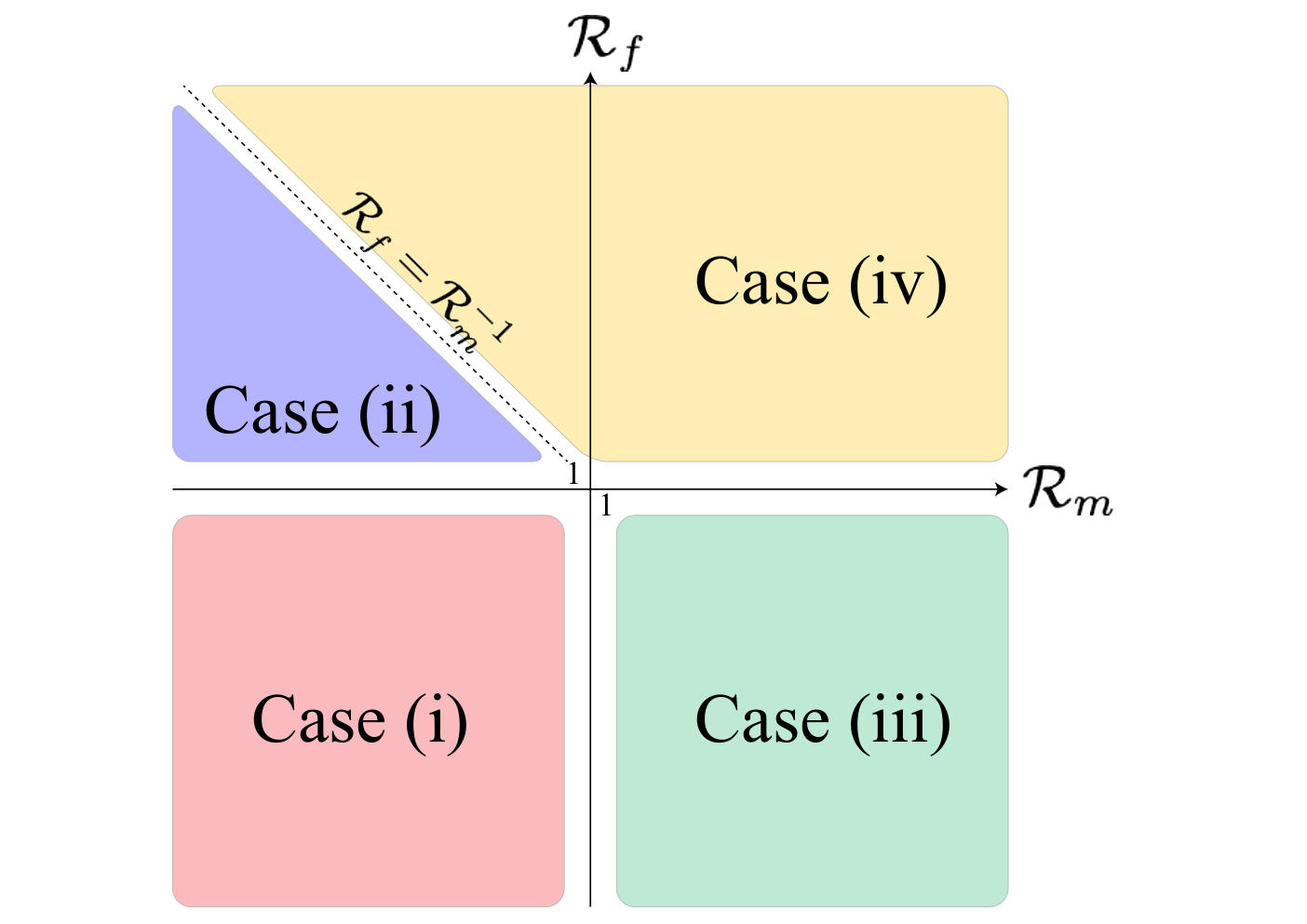
In Figs. 3 and 4, we show how the two mass eigenvalues and the mixing angle $\,\cos\xi\,$ evolve with the cosmic temperature. Among these four cases, only the case (i) exhibits a peculiar behavior that the composition of the mass eigenstates drastically changes as they evolve from high to low temperatures. Indeed, the level crossing necessarily takes places in the parameter region $\big(\mathcal{R}_{f}\ll 1\ll\mathcal{R}_{m}^{-1}\big)$ for the case (i). See Eq. (2.24). From Eqs. (2.21), (2.22) and (2.23), we see that the mixing becomes maximal at the level crossing,

$\displaystyle\cos\xi\,\big|_{T\,=\,T_{\rm lc}}=\,\frac{1}{\sqrt{2}}~,$

(2.31)

while the mixing remains small otherwise. Furthermore, the difference between the two mass eigenvalues at the level crossing reads

$\displaystyle m_{H}^{2}\big(T_{\rm lc}\big)-m_{L}^{2}\big(T_{\rm lc}\big)\,=\,2\mathcal{R}_{f}m_{\varphi}^{2}~,$

(2.32)

which becomes much smaller than $m_{a}^{2}$ and $m_{\varphi}^{2}$ for $\mathcal{R}_{f}\ll 1$ and $\mathcal{R}_{m}\ll 1$. As we will see in the next section, these properties are essential to realizing the adiabatic conversion between two mass eigenstates.

We note that, in addition to the case (i), it is worth discussing the case (ii). This is because in this case the heavy (light) axion starts to oscillate in much earlier (later) time compared to the case (i), which also leads to a non-trivial effects on the final DM abundance. We will further elaborate on this point in Sec. 3.2.

In the previous study [26], the adiabatic condition between the QCD axion and ALP was simply described without checking its validity in the whole relevant parameter space including the case in which there is a hierarchy between two decay constants $f_{a}$ and $f_{\varphi}$. In this subsection, we will generalize it based on an argument on adiabatic invariants for multiple harmonic oscillators [52] and confirm it by using the numerical analysis. To this end, let us start with the equations of motion for $a$ and $\varphi$, which are given by [26]

		$\displaystyle\ddot{a}+3H\dot{a}+m_{a}^{2}(T)f_{a}\sin\hskip-1.42271pt\bigg(\frac{a}{f_{a}}\bigg)+\frac{m_{\varphi}^{2}f_{\varphi}^{2}}{f_{a}}\sin\hskip-1.42271pt\bigg(\frac{a}{f_{a}}+\frac{\varphi}{f_{\varphi}}\bigg)\,=\,0~,$		(3.1)
		$\displaystyle\ddot{\varphi}+3H\dot{\varphi}+m_{\varphi}^{2}f_{\varphi}\sin\hskip-1.42271pt\bigg(\frac{a}{f_{a}}+\frac{\varphi}{f_{\varphi}}\bigg)\,=\,0~.$		(3.2)

Here and in what follows we focus on the evolution of the homogenous QCD axion and ALP fields in the radiation-dominated universe. For convenience, we introduce the effective angles, $\theta$ and $\Theta$, defined by

$\displaystyle\theta\,=\,\frac{a}{f_{a}}~,\quad\Theta\,=\,\frac{a}{f_{a}}+\frac{\varphi}{f_{\varphi}}~.$

(3.3)

In terms of the effective angles, the equations of motion read

		$\displaystyle\ddot{\theta}+3H\dot{\theta}+m_{a}^{2}(T)\sin\theta+m_{\varphi}^{2}{\cal R}^{2}_{f}\sin\Theta\,=\,0~,$		(3.4)
		$\displaystyle\ddot{\Theta}+3H\dot{\Theta}+m_{a}^{2}(T)\sin\theta+m_{\varphi}^{2}\Big(1+{\cal R}^{2}_{f}\Big)\sin\hskip-0.85355pt\Theta\,=\,0~,$		(3.5)

which we will numerically solve under the initial conditions, $\theta(t_{0})=\theta_{0},\Theta(t_{0})=\Theta_{0}$, and $\dot{\theta}(t_{0})=\dot{\Theta}(t_{0})=0$, where $t_{0}$ is some initial time well before the QCD axion or ALP starts to oscillate.

After the light and heavy axions start to oscillate, i.e., $H<m_{L}(T),m_{H}(T)$, the potential can be well approximated by the quadratic one since their oscillation amplitudes decrease with the cosmic expansion.⁵⁵ 5 This is not always the case. If the axion starts to oscillate at around the level crossing, the axion may go over the potential hill at the level crossing and continue to run until it is trapped by one of the potential minima, the axion roulette [27, 28]. Let us define the comoving axion numbers of the heavy and light mass eigenstates, $N_{H}$ and $N_{L}$ as

$\displaystyle N_{H}(T)\,\equiv\,\frac{\rho_{H}(T)}{m_{H}(T)s(T)}~,\quad N_{L}(T)\,\equiv\,\frac{\rho_{L}(T)}{m_{L}(T)s(T)}~,$

(3.6)

where $s(T)=2\pi^{2}g_{s}(T)T^{3}/45$ is the entropy density with $g_{s}(T)$ being the effective entropic degrees of freedom, and $\rho_{H,L}(T)$ is the energy density of the heavy or light mass eigenstate. If there were not for the mass mixing, then both $N_{H}$ and $N_{L}$ would be adiabatic invariants and so they would be separately conserved. In the presence of the mixing, however, the situation is more involved since there are multiple time scales over which the potential changes. In addition to the mass eigenvalues, the mixing angle is also time-dependent, and in particular, it exhibits a very sharp transition at the level crossing (see Fig. 4).

The time evolution of the adiabatic invariants for multiple harmonic oscillators was studied in Ref. [52]. Let $t_{\rm ext}$ denote the typical time scale over which the oscillation frequencies change significantly. The authors of Ref. [52] studied the time evolution of the quanta number of each oscillation eigenmode (like $N_{H}$ and $N_{L}$) using the Glauber variables. It was shown there that the total quanta number (which corresponds to $N_{H}+N_{L}$ in our case) is conserved if $\,t_{\rm ext}$ is much longer than the oscillation period of each eigenmode. Even in this case, each quanta number (i.e. $\hskip-2.84544ptN_{H}$ or $N_{L}$ in our case) is not necessarily conserved, if $\,t_{\rm ext}$ is shorter than or comparable to the time scale determined by the difference of the angular frequencies, i.e., the beat frequency of the two harmonic oscillators.⁶⁶ 6 The Glauber variables are the analog of the annihilation and creation operators, $(\alpha,\alpha^{*})$. They are written in terms of the canonical variables of the harmonic oscillator(s), $(q,p)$, as $\alpha\sim\sqrt{\omega}q+ip/\sqrt{\omega}$, where $\omega$ is the angular frequency. For a constant $\omega$, $\alpha$ evolves like $\alpha\sim e^{-i\omega t}$. For multiple harmonic oscillators, the quanta number of the $n$-th eigenmode is given by $\alpha_{n}^{*}\alpha_{n}$. When the angular frequencies depend on time, $d\alpha_{n}/dt$ involves terms including $\alpha_{m}$ and $\alpha_{m}^{*}$ with $m\neq n$. Therefore, the time evolution of the quanta number of the $n$-th eigenmode, $d|\alpha_{n}|^{2}/dt$, naturally involves differences between the angular frequencies, $\omega_{n}-\omega_{m}$, for $m\neq n$.

Now, let $\,t_{\rm ext}$ be the time scale over which the potential changes significantly. If there are multiple time scales, $t_{\rm ext}$ is chosen to be the shortest one among them. For example, in the case where the level crossing takes place, it is of order the Hubble time for most of the time, but it is given by the time interval for the mixing angle to change at the level crossing. In any case, $t_{\rm ext}$ is always proportional to the Hubble time, as the cosmic expansion is the only source of the time-dependence. Applying the above argument to the present case, the adiabatic condition for both $N_{H}$ and $N_{L}$ to be conserved reads

$\displaystyle t_{\rm ext}\,\gg\,\mathrm{max}\Bigg[\frac{2\pi}{m_{L}(T)},\frac{2\pi}{m_{H}(T)-m_{L}(T)}\Bigg]~.$

(3.7)

The adiabatic conversion takes place if both $N_{H}$ and $N_{L}$ are separately conserved at the level crossing. At the level crossing, $t_{\rm ext}$ is given by

$\displaystyle t_{\rm ext}\,=\,\left|\frac{1}{\cos\xi(T)}\frac{d\cos\xi(T)}{dt}\right|^{-1}_{T\,=\,T_{\text{lc}}}~.$

(3.8)

The second term in the right-handed side of Eq. (3.7) gives the dominant contribution in this case, for $\mathcal{R}_{f}\ll 1$, it reads

$\displaystyle\frac{2\pi}{m_{H}(T_{\text{lc}})-m_{L}(T_{\text{lc}})}\,\simeq\,\frac{2\pi}{\mathcal{R}_{f}m_{\varphi}}~.$

(3.9)

Using Eqs. (2.4) and (2.21), and $\mathcal{R}_{f}\ll 1$, we derive the adiabatic condition at the level crossing as

$\displaystyle\boxed{~\gamma\,\equiv\,\beta\mathcal{R}_{f}\,\sqrt{\frac{m_{\varphi}}{H(T_{\text{lc}})}}\,\gg 1\,}$

(3.10)

where we define

$\displaystyle\beta\,\equiv\,\sqrt{\frac{1}{n\pi}\scalebox{1.1}{\bigg[}1+\frac{1}{3}\frac{d\ln g_{s}(T)}{d\ln T}\scalebox{1.1}{\bigg]}}\,\Bigg|_{T\,=\,T_{\text{lc}}}~.$

(3.11)

In general, once the condition (3.7) is satisfied, we expect that both $N_{L}$ and $N_{H}$ are conserved after both the heavy and light axions start to oscillate. This is not the case if the adiabatic condition is violated. Note that here we implicitly assume that $t_{\rm ext}$ is larger than the first term $2\pi/m_{L}(T)$ [and hence $2\pi/m_{H}(T)$] in the right-handed side of Eq. (3.7) since otherwise one cannot define the numbers $N_{L}$ and $N_{H}$ unambiguously. Then, we can consider the case where $t_{\rm ext}$ becomes smaller than $2\pi/[m_{H}(T)-m_{L}(T)]$ but still larger than $2\pi/m_{L}(T)$. In this case, while the total quanta number $N_{H}+N_{L}$ is conserved, $N_{H}-N_{L}$ is not necessarily conserved. Typically this can happen at the level crossing where $m_{H}^{2}-m_{L}^{2}$ takes the minimal value and $t_{\rm ext}$ given by Eq. (3.8) becomes sufficiently small. In other words, once the condition (3.10) is violated, $N_{H}-N_{L}$ is no longer conserved at the level crossing.

In the previous work [26], the adiabatic condition was considered to be $\,m_{\varphi}/H(T_{\text{lc}})\gg 1$. However, the refined condition (3.10) contains a factor of $\,\mathcal{R}_{f}$ apart from the numerical coefficient $\beta$. This is because we have included the beat frequency in addition to the angular frequency of each mass eigenstate in the adiabatic condition. This implies that, even if $m_{\varphi}/H(T_{\text{lc}})\hskip-1.70709pt\gg\hskip-1.70709pt1$, the adiabatic condition could be broken if $\,\mathcal{R}_{f}$ is sufficiently small.

Note that the adiabatic condition (3.10) makes sense only for the parameters satisfying Eq. (2.24) (or the case (i) in the previous section), since the level crossing occurs only in this case. In the other cases (ii), (iii), and (iv) (see Fig. 2 and Table 1), the original condition (3.7) is trivially satisfied after the light and heavy axions start to oscillate. Since the level crossing does not take place in these cases, their time evolution is simple and nothing more than just the two oscillating scalar fields.

In Fig. 5, we show our numerical results of the comoving axion numbers as functions of the temperature for several choices of the parameters satisfying Eq. (2.24). In these plots, we omit the scale in the vertical axes since the overall normalization of the comoving axion number is arbitrary. As expected, the comoving axion numbers are not conserved at the level crossing when $\gamma\lesssim 1$. (Note that they are not conserved in the second panel even if $m_{\varphi}/H(T_{\text{lc}})\sim 10\gg 1$.) The adiabatic conversion takes place in the first panel. In spite of the rapid change of the mixing angle at the level crossing, the comoving axion numbers are conserved. In this case, the quantity $N_{L}\,$($N_{H}$) initially identified as the number of the QCD axion (ALP) is converted into that of the ALP (QCD axion) until the present time [see case (i) in Table 1], which affects their cosmological abundance significantly as we shall see next.

Now let us evaluate the DM abundance. In our model both the light and heavy axions could contribute to DM, and the total DM abundance is given by the sum of their contributions,

$\displaystyle\Omega_{\text{DM}}h^{2}\,=\,\Omega_{H}h^{2}+\Omega_{L}h^{2}~,\quad$

(3.12)

$\displaystyle\Omega_{H}h^{2}\,=\,\frac{m_{H}s_{0}}{\rho_{c,0}}N_{H}~,\quad\Omega_{L}h^{2}\,=\,\frac{m_{L}s_{0}}{\rho_{c,0}}N_{L}~,$

(3.13)

where $m_{H,L}\equiv m_{H,L}(T\to 0)$, and $\rho_{c,0}\,(s_{0})$ is the present critical (entropy) density. Note that $N_{H}$ and $N_{L}$ in Eq. (3.13) must be evaluated well after the level crossing since the adiabatic condition may be broken during the level crossing.

The adiabatic conversion has a significant impact on the DM abundance. Let us first consider the case (i) with $\,\mathcal{R}_{f}\ll 1$ and $\mathcal{R}_{m}\ll 1$, as the level crossing mostly takes place in this case. We focus on the evolution of the light mass eigenstate, $a_{L}$. What is peculiar is that $a_{L}$ behaves like the QCD axion before the level crossing, but it behaves like the ALP after the level crossing (see Table 1). In particular, its mass is equal to $m_{\varphi}$ in the present universe. If the adiabatic conversion takes place at the level crossing, the comoving axion number $N_{L}$ is conserved. Therefore, the contribution of $a_{L}$ to the DM abundance is smaller by the mass ratio, ${\cal R}_{m}=m_{\varphi}/m_{a}$, than without the mass mixing. This is because the QCD axion with the similar comoving number would obtain the mass $\,m_{a}$ if there were not for the mixing.

We have numerically followed the evolution of the QCD axion and ALP for a broad range of $\,{\cal R}_{f}$ and ${\cal R}_{m}$ and calculated their abundances.⁷⁷ 7 It is $m_{\varphi}$ and $f_{\varphi}$ that are actually varied in the plane of $\big({\cal R}_{m},{\cal R}_{f}\big)$ as we fix $f_{a}$ in the following. In Fig. 6, we show the contours of the DM abundance, $\Omega_{\text{DM}}h^{2}=0.12,0.5$, and 1.5 in the left panel and the contours of the relative fraction of the heavy eigenstates,

$\displaystyle r_{H}\,=\,\frac{\Omega_{H}}{\Omega_{L}+\Omega_{H}}~,$

(3.14)

in the right panel. To see if the QCD axion abundance is indeed suppressed by the mass ratio, we adopt $f_{a}=10^{13}$ GeV for which in the absence of the mass mixing the QCD axion generated by the realignment mechanism would give a too large contribution to DM unless the initial angle is smaller than unity. In other words, there would be no allowed parameter region if there were not for the mass mixing. We also adopt the initial condition $\theta_{0}=1$ and $\Theta_{0}=0$ for which $a_{H}$ is already at the potential minimum at sufficiently high temperatures.⁸⁸ 8 Precisely speaking, this is the case only if the heavy mass eigenvalue becomes equal to the Hubble parameter before the temperature-dependent axion mass $m_{a}(T)$ becomes relevant. This enables us to focus on the evolution of $a_{L}$. We shall see later how the results are modified for different initial conditions.

As one can see from the left panel of Fig. 6, there is a triangle-shaped region where one can explain DM. The region outside the blue line is excluded since the total axion abundance exceeds the observed DM abundance ($\Omega_{\text{DM}}h^{2}\simeq 0.12$). In fact, the DM is dominated by $a_{L}$ except for some region near ${\cal R}_{f}=1$ along the left boundary (see the right panel of Fig. 6). Such viable region appears (partly) due to the adiabatic conversion. We explain below how the boundary of the region is determined.

First, we notice that the viable region is fully contained in the region $\mathcal{R}_{m}<1$ and $\mathcal{R}_{f}<\mathcal{R}_{m}^{-1}$, which roughly correspond to the cases (i) and (ii). We can split the region into $\mathcal{R}_{f}<1$ (case (i)) and $\mathcal{R}_{f}>1$ (case (ii)). Let us begin with the region with $\mathcal{R}_{f}<1$. In order to suppress the axion abundance by the adiabatic conversion, the mass ratio $\,\mathcal{R}_{m}$ needs to be less than unity. If we decrease the value of $\,\mathcal{R}_{m}$ from unity for fixed $\mathcal{R}_{f}\,(<1)$, at some point the suppression becomes sufficient to explain the observed DM abundance. This corresponds to the right vertical contours shown in the left panel of Fig. 6. Then, if we further decrease the value of $\mathcal{R}_{m}$, the abundance becomes more suppressed, but at a certain point, the adiabatic condition becomes violated, since $\,\gamma\,$ defined in Eq. (3.10) decreases as $\,m_{\varphi}$ decreases for fixed ${\cal R}_{f}$. (Note that $H(T_{\rm lc})$ increases as $\,m_{\varphi}$ decreases.) Once the adiabatic condition is broken, $N_{L}$ is no longer conserved, and its large fraction is converted to $N_{H}$. For the adopted parameters, the production of the heavy mode leads to the DM overproduction, which explains the bottom-left part of the contours. Indeed, the bottom-left boundary runs in parallel with the line of $\gamma=1$, below which the adiabatic condition is violated. The production of the heavy mode in the region $\gamma<1$ can also be seen in the right panel of Fig. 6.

Next, let us consider the region with $\mathcal{R}_{f}>1$. In this case, the level crossing does not take place and the adiabatic condition is trivial. In other words, $N_{H}$ and $N_{L}$ are separately conserved after both axions start to oscillate. Therefore, it is important to know when and how much those heavy and light axions are produced.

We start with the upper-right region of the triangle-shaped boundary. The heavy mass eigenvalue is given by ${\cal R}_{f}m_{\varphi}$ at high temperatures, and it grows as $m_{a}(T)$ at low temperatures. They satisfy ${\cal R}_{f}m_{\varphi}<m_{a}$ in the region we consider. Near the upper-right boundary, the heavy axion mass becomes equal to the Hubble parameter well before the temperature-dependent axion mass, $m_{a}(T)$, turns on. For the present choice of the initial condition, the heavy axion already sits at the potential minimum (in the limit of $m_{a}(T)\to 0$), and so, the heavy axion has a negligible abundance. This can also be seen in the right panel of Fig. 6. So let us focus on the light axion whose mass evolves as ${\cal R}_{f}^{-1}m_{a}(T)$ at high temperatures, and asymptotes to $\,m_{\varphi}$ at low temperatures. When the light axion mass becomes comparable to the Hubble parameter, the light axion starts to oscillate. Let us denote as $H_{\rm osc}$ the Hubble parameter at the onset of the oscillation. Afterwards, $N_{L}\propto H_{\rm osc}^{-1/2}\hskip-1.42271ptf_{\varphi}^{2}\,$ is conserved. Therefore, the DM abundance is proportional to $m_{\varphi}H_{\rm osc}^{-1/2}\hskip-1.42271ptf_{\varphi}^{2}\propto m_{\varphi}f_{\varphi}^{(2n+5)/(n+2)}$, where $n=4.08$ is given in Eq. (2.4). This explains the dependence of the upper-right boundary, ${\cal R}_{f}\propto{\cal R}_{m}^{-0.46}$.

Finally, let us consider what happens if one decreases $\,{\cal R}_{m}$ from the upper-right boundary for a fixed ${\cal R}_{f}$. In this case, the heavy axion mass becomes lighter, and at a certain point, it becomes equal to the Hubble parameter after the QCD axion mass turns on. So it starts to oscillate when $m_{a}(T)\sim H$, and it oscillates along the QCD axion $a$. For $f_{a}=10^{13}$ GeV, thus produced QCD axion exceeds the observed DM abundance for the oscillation amplitude of order unity, and therefore, there will be no allowed region once the heavy axion starts to oscillate when $m_{a}(T)\hskip-1.42271pt\sim\hskip-1.42271ptH$. The critical point is where $\,{\cal R}_{f}m_{\varphi}\sim m_{a}(T)\sim H$. Since the middle and right-handed side of this relation are independent of $f_{\varphi}$ or $m_{\varphi}$, the upper-left boundary satisfies ${\cal R}_{f}\hskip-1.70709pt\propto\hskip-1.70709pt{\cal R}_{m}^{-1}$. Around the critical point, the heavy axion is slightly produced by the realignment mechanism explained above. Since the boundary is determined by the heavy axion abundance, it sensitively depends on the initial condition in contrast to the other boundaries. We will see below how this boundary is modified for different initial conditions.

In the right panel of Fig. 6, we show the contours of $\,r_{H}=0.99,0.9$, and $0.1$, as well as the contour of $\,\Omega_{\rm DM}=0.12$ (orange dashed line). The region outside the orange dashed line is excluded since the total axion abundance exceeds the observed DM abundance. If one looks at the left-boundary of the dashed line, one can see that the fraction of the heavy axion increases from $0.1$ to $0.9$ as $\,{\cal R}_{f}$ increases to unity, and then decreases from $0.9$ to $0.1$ as $\,{\cal R}_{f}$ further increases from unity. This behavior may be understood as follows.⁹⁹ 9 While our estimate on the axion abundance could be modified near $\,{\cal R}_{f}=1$ as this is the boundary of the cases (i) and (ii), the interpretation given here should hold when ${\cal R}_{f}$ much larger or smaller than unity. For $\,{\cal R}_{f}\lesssim 1$, the light axion abundance becomes more suppressed as $\,{\cal R}_{m}$ decreases, and so, the heavy axion needs to compensate it to explain the observed DM abundance. This explains why $r_{H}$ increases along the orange dashed line as ${\cal R}_{f}$ increases (or ${\cal R}_{m}$ decreases). On the other hand, for ${\cal R}_{f}\gtrsim 1$, the light axion abundance is proportional to $m_{\varphi}f_{\varphi}^{(2n+5)/(n+2)}$, which increases along the orange dashed line which scales as ${\cal R}_{f}\propto{\cal R}_{m}^{-1}$. Therefore, the heavy axion fraction decreases along the orange dashed line as ${\cal R}_{f}$ increases (or $\,{\cal R}_{m}$ decreases). The heavy axion can be produced either by the weak violation of the adiabatic condition or by a small contribution of the realignment mechanism.

In Fig. 7 we show the contours of $\,\Omega_{\rm DM}h^{2}=0.12\,$ for different values of $f_{a}=(3,5,10)\times 10^{12}$ GeV. The region expands as $f_{a}$ decreases since the required suppression of the DM abundance becomes smaller.

We show the contour of $\Omega_{\rm DM}h^{2}=2$ for different initial angles in Fig. 8. To ease the comparison we choose such initial angles that only the heavy axion is varied, while the light one along the minimum of the potential (2.12) remains the same. This is realized by varying $\Theta_{0}$ with $\,\theta_{0}=1+\big[{\cal R}_{f}^{2}/\big(1+{\cal R}_{f}^{2}\big)\big]\Theta_{0}$. As one can see from Fig. 8, the boundaries are almost the same for the three cases where they are determined by the light axion abundance. The exception is the left boundary with ${\cal R}_{f}>1$ where it is determined by the heavy axion abundance. For $\Theta_{0}=0.3$, the heavy axion abundance increases relative to $\Theta_{0}=0$, since its effective amplitude is determined by $\theta_{0}$. For $\Theta_{0}=-\,0.3$, the heavy axion abundance decreases relative to $\Theta_{0}=0$, and the total abundance falls short of $\,\Omega_{\rm DM}h^{2}=2$. This explains the behavior of the blue dotted line in Fig. 8. In the region between the blue dotted lines, the DM abundance is approximately constant, and it is given by $\,\Omega_{\rm DM}h^{2}\simeq 1.2$. This is because the DM is dominated by the heavy axion, i.e. the QCD axion whose abundance is independent of $\,m_{\varphi}$ and $f_{\varphi}$. With the same initial angles and the decay constant $f_{a}$, we have also confirmed that the boundaries of the contours of $\,\Omega_{\rm DM}h^{2}=0.12$ are mostly insensitive to the choice of initial angles except for a slight change in the left boundary with ${\cal R}_{f}>1$. Therefore, our results are robust against the choice of different initial angles.

In summary, the dynamics of the QCD axion and ALP in the presence of the mass mixing suppresses the DM abundance, which can expand the viable parameter space. There are two possibilities to realize the suppression of the DM abundance: One is the case where the level crossing takes place and ALP is produced by the adiabatic conversion of the QCD axion, which corresponds to the case (i) in Table 1. The other is the case where the heavy and light axions undergo a non-trivial time evolution without level crossing, which corresponds to the case (ii) in Table 1. In particular, even for a moderately large QCD axion decay constant which usually leads to the overproduction of the QCD axion by the realignment mechanism, there appears a viable parameter region where one can explain the observed DM. For this, the ALP mass must be smaller than the QCD axion mass, while the ALP decay constant can be a few orders of magnitude smaller than the QCD axion.

References

- [1] B. Graner, Y. Chen, E. G. Lindahl and B. R. Heckel, Phys. Rev. Lett. 116, no. 16, 161601 (2016) Erratum: [Phys. Rev. Lett. 119, no. 11, 119901 (2017)] [arXiv:1601.04339 [physics.atom-ph]].
- [2] R. D. Peccei and H. R. Quinn, Phys. Rev. Lett. 38, 1440 (1977).
- [3] R. D. Peccei and H. R. Quinn, Phys. Rev. D 16, 1791 (1977).
- [4] S. Weinberg, Phys. Rev. Lett. 40, 223 (1978).
- [5] F. Wilczek, Phys. Rev. Lett. 40, 279 (1978).
- [6] G. ’t Hooft, Phys. Rev. Lett. 37, 8 (1976).
- [7] E. Witten, Nucl. Phys. B 156, 269 (1979).
- [8] G. Veneziano, Nucl. Phys. B 159, 213 (1979).
- [9] J. Preskill, M. B. Wise and F. Wilczek, Phys. Lett. B 120, 127 (1983).
- [10] L. F. Abbott and P. Sikivie, Phys. Lett. B 120, 133 (1983).
- [11] M. Dine and W. Fischler, Phys. Lett. B 120, 137 (1983).
- [12] A. Arvanitaki, S. Dimopoulos, S. Dubovsky, N. Kaloper and J. March-Russell, Phys. Rev. D 81, 123530 (2010) [arXiv:0905.4720 [hep-th]].
- [13] B. S. Acharya, K. Bobkov and P. Kumar, JHEP 1011, 105 (2010) [arXiv:1004.5138 [hep-th]].
- [14] M. Cicoli, M. Goodsell and A. Ringwald, JHEP 1210, 146 (2012) [arXiv:1206.0819 [hep-th]].
- [15] D. Cadamuro and J. Redondo, JCAP 1202, 032 (2012) [arXiv:1110.2895 [hep-ph]].
- [16] P. Arias, D. Cadamuro, M. Goodsell, J. Jaeckel, J. Redondo and A. Ringwald, JCAP 1206, 013 (2012) [arXiv:1201.5902 [hep-ph]].
- [17] J. E. Kim and G. Carosi, “Axions and the Strong CP Problem,” Rev. Mod. Phys. 82, 557 (2010) [arXiv:0807.3125 [hep-ph]].
- [18] O. Wantz and E. P. S. Shellard, “Axion Cosmology Revisited,” Phys. Rev. D 82, 123508 (2010) [arXiv:0910.1066 [astro-ph.CO]].
- [19] A. Ringwald, “Exploring the Role of Axions and Other WISPs in the Dark Universe,” Phys. Dark Univ. 1, 116 (2012) [arXiv:1210.5081 [hep-ph]].
- [20] M. Kawasaki and K. Nakayama, “Axions: Theory and Cosmological Role,” Ann. Rev. Nucl. Part. Sci. 63, 69 (2013) [arXiv:1301.1123 [hep-ph]].
- [21] D. J. E. Marsh, “Axion Cosmology,” Phys. Rept. 643, 1 (2016) [arXiv:1510.07633 [astro-ph.CO]].
- [22] I. G. Irastorza and J. Redondo, Prog. Part. Nucl. Phys. 102, 89 (2018) [arXiv:1801.08127 [hep-ph]].
- [23] T. Higaki and F. Takahashi, JHEP 1407, 074 (2014) [arXiv:1404.6923 [hep-th]].
- [24] T. Higaki and F. Takahashi, Phys. Lett. B 744, 153 (2015) [arXiv:1409.8409 [hep-ph]].
- [25] C. T. Hill and G. G. Ross, Nucl. Phys. B 311, 253 (1988).
- [26] N. Kitajima and F. Takahashi, JCAP 1501, no. 01, 032 (2015) [arXiv:1411.2011 [hep-ph]].
- [27] R. Daido, N. Kitajima and F. Takahashi, Phys. Rev. D 92, no. 6, 063512 (2015) [arXiv:1505.07670 [hep-ph]].
- [28] R. Daido, N. Kitajima and F. Takahashi, Phys. Rev. D 93, no. 7, 075027 (2016) [arXiv:1510.06675 [hep-ph]].
- [29] L. Wolfenstein, Phys. Rev. D 17, 2369 (1978).
- [30] S. P. Mikheev and A. Y. Smirnov, Sov. J. Nucl. Phys. 42, 913 (1985) [Yad. Fiz. 42, 1441 (1985)].
- [31] S. P. Mikheev and A. Y. Smirnov, Nuovo Cim. C 9, 17 (1986).
- [32] G. Grilli di Cortona, E. Hardy, J. Pardo Vega and G. Villadoro, JHEP 1601, 034 (2016) [arXiv:1511.02867 [hep-ph]].
- [33] S. Borsanyi et al., Nature 539, no. 7627, 69 (2016) [arXiv:1606.07494 [hep-lat]].
- [34] E. Berkowitz, M. I. Buchoff and E. Rinaldi, Phys. Rev. D 92, no. 3, 034507 (2015) [arXiv:1505.07455 [hep-ph]].
- [35] P. Petreczky, H. P. Schadler and S. Sharma, Phys. Lett. B 762, 498 (2016) [arXiv:1606.03145 [hep-lat]].
- [36] J. Frison, R. Kitano, H. Matsufuru, S. Mori and N. Yamada, JHEP 1609, 021 (2016) [arXiv:1606.07175 [hep-lat]].
- [37] Y. Taniguchi, K. Kanaya, H. Suzuki and T. Umeda, Phys. Rev. D 95, no. 5, 054502 (2017) [arXiv:1611.02411 [hep-lat]].
- [38] C. Bonati, M. D’Elia, M. Mariti, G. Martinelli, M. Mesiti, F. Negro, F. Sanfilippo and G. Villadoro, JHEP 1603, 155 (2016) [arXiv:1512.06746 [hep-lat]].
- [39] T. Hiramatsu, M. Kawasaki, K. Saikawa and T. Sekiguchi, Phys. Rev. D 85, 105020 (2012) Erratum: [Phys. Rev. D 86, 089902 (2012)] [arXiv:1202.5851 [hep-ph]].
- [40] M. Kawasaki, K. Saikawa and T. Sekiguchi, Phys. Rev. D 91, no. 6, 065014 (2015) [arXiv:1412.0789 [hep-ph]].
- [41] L. Fleury and G. D. Moore, JCAP 1601, 004 (2016) [arXiv:1509.00026 [hep-ph]].
- [42] V. B. Klaer and G. D. Moore, JCAP 1711, no. 11, 049 (2017) [arXiv:1708.07521 [hep-ph]].
- [43] M. Gorghetto, E. Hardy and G. Villadoro, JHEP 1807, 151 (2018) [arXiv:1806.04677 [hep-ph]].
- [44] M. Kawasaki, T. Sekiguchi, M. Yamaguchi and J. Yokoyama, arXiv:1806.05566 [hep-ph].
- [45] G. Ballesteros, J. Redondo, A. Ringwald and C. Tamarit, JCAP 1708, no. 08, 001 (2017) [arXiv:1610.01639 [hep-ph]].
- [46] T. Kobayashi, R. Kurematsu and F. Takahashi, JCAP 1309, 032 (2013) [arXiv:1304.0922 [hep-ph]].
- [47] P. W. Graham and A. Scherlis, Phys. Rev. D 98, no. 3, 035017 (2018) [arXiv:1805.07362 [hep-ph]].
- [48] F. Takahashi, W. Yin and A. H. Guth, Phys. Rev. D 98, no. 1, 015042 (2018) [arXiv:1805.08763 [hep-ph]].
- [49] R. Mayle, J. R. Wilson, J. R. Ellis, K. A. Olive, D. N. Schramm and G. Steigman, Phys. Lett. B 203, 188 (1988).
- [50] G. Raffelt and D. Seckel, Phys. Rev. Lett. 60, 1793 (1988).
- [51] M. S. Turner, Phys. Rev. Lett. 60, 1797 (1988).
- [52] M. Devaud, V. Leroy, J-C. Bacri, and T. Hocquet, https://hal.archives-ouvertes.fr/hal-00197565, 2007.
- [53] S. J. Asztalos et al. [ADMX Collaboration], Phys. Rev. D 69, 011101 (2004) [astro-ph/0310042].
- [54] S. J. Asztalos et al. [ADMX Collaboration], Phys. Rev. Lett. 104, 041301 (2010) [arXiv:0910.5914 [astro-ph.CO]].
- [55] G. Carosi, A. Friedland, M. Giannotti, M. J. Pivovaroff, J. Ruz and J. K. Vogel, arXiv:1309.7035 [hep-ph].
- [56] V. Anastassopoulos et al. [CAST Collaboration], Nature Phys. 13 (2017) 584 [arXiv:1705.02290 [hep-ex]].
- [57] https://indico.in2p3.fr/event/16579/contributions/60840/attachments/47276/59399/Moriond.pdf
- [58] E. Petrakou [CAPP/IBS Collaboration], EPJ Web Conf. 164, 01012 (2017) [arXiv:1702.03664 [physics.ins-det]].
- [59] A. Caldwell et al. [MADMAX Working Group], Phys. Rev. Lett. 118, no. 9, 091801 (2017) [arXiv:1611.05865 [physics.ins-det]].
- [60] Y. Kahn, B. R. Safdi and J. Thaler, Phys. Rev. Lett. 117, no. 14, 141801 (2016) [arXiv:1602.01086 [hep-ph]].
- [61] R. Bähre et al., JINST 8, T09001 (2013) [arXiv:1302.5647 [physics.ins-det]].
- [62] E. Armengaud et al., JINST 9, T05002 (2014) [arXiv:1401.3233 [physics.ins-det]].
- [63] A. Ayala, I. Domínguez, M. Giannotti, A. Mirizzi and O. Straniero, Phys. Rev. Lett. 113, no. 19, 191302 (2014) [arXiv:1406.6053 [astro-ph.SR]].
- [64] J. E. Kim, Phys. Rev. Lett. 43, 103 (1979).
- [65] M. A. Shifman, A. I. Vainshtein and V. I. Zakharov, Nucl. Phys. B 166, 493 (1980).
- [66] M. Dine, W. Fischler and M. Srednicki, Phys. Lett. 104B, 199 (1981).
- [67] A. R. Zhitnitsky, Sov. J. Nucl. Phys. 31, 260 (1980) [Yad. Fiz. 31, 497 (1980)].
- [68] P. A. R. Ade et al. [Planck Collaboration], Astron. Astrophys. 594, A20 (2016) [arXiv:1502.02114 [astro-ph.CO]].
- [69] T. Higaki, K. S. Jeong, N. Kitajima, T. Sekiguchi and F. Takahashi, JHEP 1608, 044 (2016) [arXiv:1606.05552 [hep-ph]].
- [70] A. J. Long, arXiv:1803.07086 [hep-ph].
- [71] T. Higaki, K. S. Jeong, N. Kitajima and F. Takahashi, Phys. Lett. B 755, 13 (2016) [arXiv:1512.05295 [hep-ph]].
- [72] T. Higaki, K. S. Jeong, N. Kitajima and F. Takahashi, JHEP 1606, 150 (2016) [arXiv:1603.02090 [hep-ph]].