Accounting for phenology in the analysis of animal movement–3.6.1 \artmonthFebruary
Accounting for phenology in the analysis of animal movement
Abstract
The analysis of animal tracking data provides important scientific understanding and discovery in ecology. Observations of animal trajectories using telemetry devices provide researchers with information about the way animals interact with their environment and each other. For many species, specific geographical features in the landscape can have a strong effect on behavior. Such features may correspond to a single point (e.g., dens or kill sites), or to higher-dimensional subspaces (e.g., rivers or lakes). Features may be relatively static in time (e.g., coastlines or home-range centers), or may be dynamic (e.g., sea ice extent or areas of high-quality forage for herbivores). We introduce a novel model for animal movement that incorporates active selection for dynamic features in a landscape. Our approach is motivated by the study of polar bear (Ursus maritimus) movement. During the sea ice melt season, polar bears spend much of their time on sea ice above shallow, biologically productive water where they hunt seals. The changing distribution and characteristics of sea ice throughout the year means that the location of valuable habitat is constantly shifting. We develop a model for the movement of polar bears that accounts for the effect of this important landscape feature. We introduce a two-stage procedure for approximate Bayesian inference that allows us to analyze over 300,000 observed locations of 186 polar bears from 2012–2016. We use our model to estimate a spatial boundary of interest to wildlife managers that separates two sub-populations of polar bears from the Beaufort and Chukchi seas.
keywords
animal movement; resource selection function; sea ice; Ursus maritimus;1 Introduction
For decades, study of animal movement has led to important scientific understanding and discoveries in ecology (Hooten et al., 2017). Observations of animal trajectories using telemetry devices, such as radio collars, have provided researchers with information about the way animals interact with their environment (e.g., Manly et al. 2002; Johnson et al. 2008) and each other (Niu et al., 2016; Scharf et al., 2016; Scharf et al., 2018, e.g.,). In the case of the former, one of the most common approaches used by ecologists is to analyze the rates at which animals use certain types of habitats relative to the distribution of habitat types available to them (Manly et al. 2002; Lele and Keim 2006; Hooten et al. 2017). Such analyses typically model the probability of an individual using a particular location as a weighted combination of all available locations (Johnson et al., 2006; Northrup et al., 2013, e.g.,). The weights are then referred to as the resource selection function (RSF) and provide insight into which portions of a landscape are most valuable to the study species. What constitutes an available location depends on the characteristics of the particular species under study and the rate at which telemetry observations are gathered.
For many species, specific geographical features in the landscape can have a strong effect on where individuals choose to move (Tracey et al., 2005). Such features are sometimes well-summarized by a single point (e.g., dens or kill sites), but may also correspond to higher-dimensional subspaces (e.g., rivers or lakes). Their locations may be relatively static in time (e.g., coastlines or home range centers in Brost et al. 2016), or may be dynamic, potentially varying periodically (e.g., sea ice extent or areas of high-quality forage for herbivores). The term pheonology is used to refer to those characteristics of an ecosystem that demonstrate seasonal patterns of variation. While not always framed in the context of resource selection, these landscape features can nevertheless be thought of as resources, and the behavior of animals may demonstrate selection for (or against) points near the feature. We introduce a novel suite of models for the analysis of animal movement that incorporates active selection for features in a landscape that may have complex and dynamic shapes.
Our modeling framework is motivated by the study of polar bear (Ursus maritimus) movement. Polar bears spend much of their time on sea ice over shallow, biologically productive water where they hunt ringed seals (Pusa hispida). The distribution of this primary food source can be highly variable and is known to depend on a wide variety of factors including season, bathymetry, and various characteristics of the sea ice (Kelly et al., 2010, e.g.,). Ringed seals depend heavily on sea ice throughout their lives and use both fast ice (ice that is connected to land) and pack ice (ice that is free to drift) (Finley et al., 1983; Wiig et al., 1999, e.g.,) for feeding, rearing pups, and molting. A consistent pattern across multiple studies is that some of the most valuable habitat for ringed seals, and hence polar bears, is near the interface between sea ice and the ocean (Frost et al., 2004; Durner et al., 2009; Crawford et al., 2012; Rode et al., 2015; Atwood et al., 2016) especially during the sea ice melt season, the part of the year when sea ice first breaks up and contracts toward the pole, then freezes and expands southward again. The changing distribution and characteristics of sea ice throughout the late spring through early fall means that the location of valuable ice-edge habitat is constantly shifting.
As climate change alters the rate at which sea ice thaws and freezes, as well as the size of its minimum and maximum extents, there is increasing concern about how polar bears are responding to these dramatic shifts in their environment (Rode et al., 2014). Our goal is to develop a model for the movement of polar bears that explicitly accounts for the effect of the changing sea ice and can be incorporated into a wide variety of hierarchical models used to better understand polar bear ecology. In Section 3, we use our model to estimate a spatial boundary of interest to wildlife managers that separates two sub-populations of polar bears from the Beaufort and Chukchi seas.
2 Model Development
2.1 Feature preference
To account for an individual’s preference for areas in a landscape near (or far from) a particular feature of interest, we take a use-availability approach. We define the selection weight of a particular location to be a parametric function of the distance from the location to a feature of interest on the landscape. Estimates of the relevant parameters provide a summary of how strongly the feature affects the behavior of observed individuals. We model availability similar to Hjermann (2000), Christ et al. (2008), Johnson et al. (2008), and Brost et al. (2015) who used radial distributions centered on the most recently-observed location to define the continuously-valued availability at each point in time.
Let be the location of an individual at time , where we assume for now that observation times are equally spaced with no missing values. We define the conditional probability density for as
| (1) |
where we use square brackets to denote a probability density, and denotes the normal probability density function with mean and variance evaluated at . For , the conditional distribution is proportional to the product of two components, the first of which is the density of a bivariate Gaussian distribution centered on the previous location of the individual, and defines the availability of each point on the landscape as in Christ et al. (2008). The availability component induces positive auto-correlation in the joint process , with larger values of resulting in processes with greater distances between consecutive locations and faster, more erratic movement.
The function is a RSF and controls the effect a particular feature in the landscape has on an individual’s movement. Let denote the set of points that comprise the feature of interest (e.g., the interface between sea ice and ocean). We define the function as
| (2) |
(where is the or Euclidean norm) so that the value of is highest near , and drops to zero as moves away from . The value of controls the range at which effectively reduces to zero. We show in Section 2.2 why this particular parametric form for the RSF can be used to leverage computational efficiencies in parameter estimation.
In practice, it will often be useful to define such that it achieves its largest values at locations near so that the conditional density given in (1) has probability mass concentrated near . Specifying in this way provides a method for modeling movement that exhibits preference for the region of the landscape near the feature of interest.
The model for the discrete-time continuous-space process provides a useful tool for modeling the movement of an individual responding to a one-dimensional feature on a landscape. In Section 3, we apply the model to the movement of polar bears with the ultimate goal of clustering individuals into disjoint sub-populations based on space use. By including availability and resource selection as part of a larger hierarchical structure, we are able to account for polar bears preference for habitats that facilitate the depredation of seals, which, if ignored, might result in biased inference about sub-population membership.
The conditional density in (1) is only defined up to a constant of proportionality, , that must be computed as part of any likelihood-based estimation procedure. We employ a Bayesian hierarchical methodology and fit our model for polar bear movement using Markov chain Monte Carlo (MCMC), which requires computation of the normalizing constant several times at each iteration of the algorithm. For a general feature, , the normalization constant is not analytically tractable. Thus, some form of numerical integration is required to fit the model to data, the computational cost of which precludes such an approach in our application. In the RSF literature, the normalization constant has typically been approximated using either a coarse spatial discretization (e.g., Warton and Shepherd 2010; Brost et al. 2015), or a randomized scheme based on an “availability sample” (Northrup et al., 2013, e.g.,). In the next section, we introduce a novel and computationally efficient approach for computing the necessary normalization constant that leverages conjugacy in the distributional form for .
2.2 Linearization approximation
We implement a novel approximation technique that assumes locally linear structure in the shape of , allowing for efficient approximation of the true conditional density of . To motivate our approximation, we note that, for the special case when is a straight line, the RSF as defined in (2) can be written in a form similar to that of a bivariate Gaussian density function with a rank-deficient covariance matrix.
2.2.1 RSF for straight lines
First, we consider the case of a vertical line, , in the real plane so that . For this case, we have
for all real-valued . To allow for that are straight, but not necessarily vertically oriented, we rotate the coordinate system through an angle . Let be the rotation matrix defined as and let be defined such that for some real-valued . Note that the inverse of a rotation matrix, , is also equal to its transpose, . The RSF defined in (2) is invariant under rigid transformations such as rotations, therefore
2.2.2 Linearizing complex landscape features
The resulting form for is proportional to the product of two Gaussian distributions, one of which is improper. Provided , the product is a proper bivariate Gaussian distribution with mean, and covariance, , where is any point in . The distributional form of implicitly defines the appropriate normalization constant in (1). Thus, if there exists some straight line that represents a close approximation to near , then may provide a reasonable approximation for that alleviates the computational burden of repeatedly calculating the necessary normalization constant. A natural candidate for is the line that is tangent to at the point on closest to , because this is the portion of the feature most relevant to the conditional distribution of .

Let be the point in nearest to , and let be the set of points that lie on the line tangent to at . Figure 1 shows a schematic illustrating the way the product of the two Gaussian components in (1) combine to result in a third Gaussian distribution. For to result in an adequate approximation of the RSF, the linearized feature need only resemble the true feature in the vicinity of . Outside of the immediate neighborhood, the availability distribution will be essentially zero, reducing the impact of errors in the RSF approximation. We discuss the appropriateness of the linearization approximation in greater detail and offer practical guidance for its use in future studies in Supporting Information D.
3 Application
3.1 Goals and previous work
There are a total of 19 recognized polar bear sub-populations in the circumpolar Arctic (Obbard et al., 2010, Figure 2,). However, the boundaries that delineate the sub-populations are challenging to precisely define because there are few barriers to movement for polar bears, and the changing extent and drift of the sea ice leads to periods of the year when individuals from different sub-populations may use overlapping portions of the landscape. Nevertheless, there are important reasons to determine a clear delineation of the sub-population boundaries. For example, wildlife management agencies such as the U.S. Fish and Wildlife Service (USFWS) use sub-population boundaries to help guide management decisions for polar bears, which are currently listed as ‘threatened’ under the Endangered Species Act (U.S. Fish and Wildlife, 2016). There is also evidence that polar bears from different sub-populations are responding to climate change with differing degrees of success (Rode et al., 2014; Ware et al., 2017). Statistical methods that make use of polar bear movement data have been used to estimate these boundaries in the past (Amstrup et al., 2005). In what follows, we focus on demonstrating how our model may be used for estimating a sub-population boundary between the Chukchi Sea (CS) and Southern Beaufort Sea (SB) sub-populations. We compare previous statistical approaches with our proposed methodology in Supporting Information A.

3.2 Movement process model
With the exception of mothers denning on land, most polar bears remain on the ice in the summer, following it north as it retreats away from continental land masses. Polar bears are specialist carnivores that use areas near the interface of sea ice and ocean to hunt seals during the sea ice melt season (Durner et al., 2009). However, some polar bears do remain on land through the warmest part of the year and, in fact, Atwood et al. (2016) concluded that there is evidence the number of individuals exhibiting this behavior is increasing.
Two of the primary characteristics of polar bear movement are a tendency for most individuals to prefer portions of the landscape near the edge of the sea ice (Durner et al., 2004; Ware et al., 2017), and a tendency for individuals to occupy a general spatial region corresponding to the particular unobserved sub-population to which an individual polar bear is a member. To address the effect of the sea ice, we specify a model for movement that incorporates preference for areas near the sea ice boundary as it changes in time. We account for polar bears that remain on land during the summer by also including coastline as a feature on the landscape associated with increased rates of use, as individuals that spend the summer on land tend to remain on islands and/or near the coastline for most of the season (Rode et al., 2015). By accounting for habitat variability, we hope to avoid inadvertently clustering bears into sub-populations that confound true sub-population spatial regions with movement responding to changing sea ice.
We take a Bayesian hierarchical modeling perspective, allowing us to specify models for both measurement error and the true unobserved movement process in a single coherent framework. We use a discrete-time approach to specify a model for polar bear movement, in which the conditional probability density for the location of an individual is proportional to a product of components corresponding to resource availability and selection. The discrete-time approach is motivated by the scale at which we have measurements of Arctic sea ice, which features as a direct effect in our model for movement. We use estimates of the extent of sea ice provided by the National Snow and Ice Data Center (Fetterer et al., 2010) that are available at daily intervals at 4km resolution; thus, we model movement as a discrete-time stochastic process on a daily scale.
Let denote the location of individual at time , where is a consecutive set of times from the reference set , and let be a binary random variable that equals 1 if individual belongs to the CS sub-population, and 0 if it belongs to the SB sub-population (for the general case of more than two sub-populations, may be specified as a categorical variable coming from a multinomial distribution). Additionally, we denote by the set of points in the plane defined by the union of coast line, and the edge of the sea ice. Figure 5 in Supporting Information A shows realizations of the dynamic feature of interest, , for three days in 2018. We model the conditional distribution of as
| (3) |
Each component in (3) captures a different feature of the movement process. Namely, these are (i) the association of each individual bear with a sub-population-level central place, (ii) the temporal dependence between locations on consecutive days, and (iii) a RSF that appropriately weights locations near a coastline or the edge of the sea ice. The first two terms can be thought of as a two-component availability function that incorporates a sub-population activity center and movement constraints, similar in many respects to the modeling specification of Christ et al. (2008) and Johnson et al. (2008). The third term is a RSF that models the preference polar bears exhibit for habitat near either a coastline, or the sea ice boundary. The exponents in components (ii) and (iii) are indicator functions that remove those effects at the initial time point for which we assume the only information we have about an individual’s location comes from their association with a particular sub-population.
3.3 Activity centers and sub-population membership
The second component in (3), for , and first component for is a bivariate Gaussian distribution centered on one of two central places, and , corresponding to the centers of the SB and CS sub-populations, respectively. The covariance matrices, and , control the strength of the effect the sub-population center has on the movement of each individual. As the marginal variances of and increase, individuals are allowed to range farther from their central place. We specify prior distributions for and based on their spectral decompositions. Details are provided in Supporting Information B.
The binary random variables, , indicate the particular sub-population with which individual associates. We specify Bernoulli prior distributions for each with probability 0.5, corresponding to balanced a priori classification of each individual.
3.4 Time-varying RSF
For the application to polar bear movement, we modified the RSF introduced in (2) slightly to account for an important aspect of polar bear ecology. Polar bears’ preference for habitat near the coastlines and boundary between ocean and sea ice can vary seasonally throughout the year. Previous analyses of polar bear movement concluded that the preference for habitat near the sea ice boundary is highest during summer and autumn months and weakest in the spring (Durner et al., 2004; Durner et al., 2009; Wilson et al., 2016). Thus, we defined a RSF with the same shape characteristics as in (2), but with an added indicator function that accounts for the difference in seasons when the landscape feature is most relevant, and when it has negligible impact on movement. Let and denote the days of the year on which this “summer” season begins and ends, respectively. Then the modified RSF was defined as
| (4) |
We specified Gaussian prior distributions for the end-points of the “summer” such that , , corresponding to prior start and end date distributions with means of May 15 and November 15, respectively, and a standard deviation of two weeks.
One way to interpret this generalization of (2) is to define the RSF in the original way, but let vary in time. The modified RSF given by (4) arises for the case of a dynamic parameter that is constant and finite during the “summer” season, and infinite during the rest of the year. Thus, outside of the season defined by the landscape feature defined by has no effect on movement.
3.5 Measurement error
We analyzed telemetry observations of polar bears made by the USFWS (USFWS unpublished data) and the U.S. Geological Survey (USGS) (USGS unpublished data) using a variety of different telemetry device types contaminated with measurement error of varying severity. All locations were projected to a grid using an Albers equal area projection, with all distances measured in kilometers. In each case, we model the observed locations as centered on the true, unobserved location of the individual with an additive measurement error process as , where the distribution for depends on the particular device used to make the observation , and we allow measurements to be made at any point on the continuous interval . We provide full details related to the measurement error model and address the misalignment between this continuous-time scale and the discrete scale used to model the movement process in Supporting Information B.
3.6 Results
3.6.1 Sub-populations
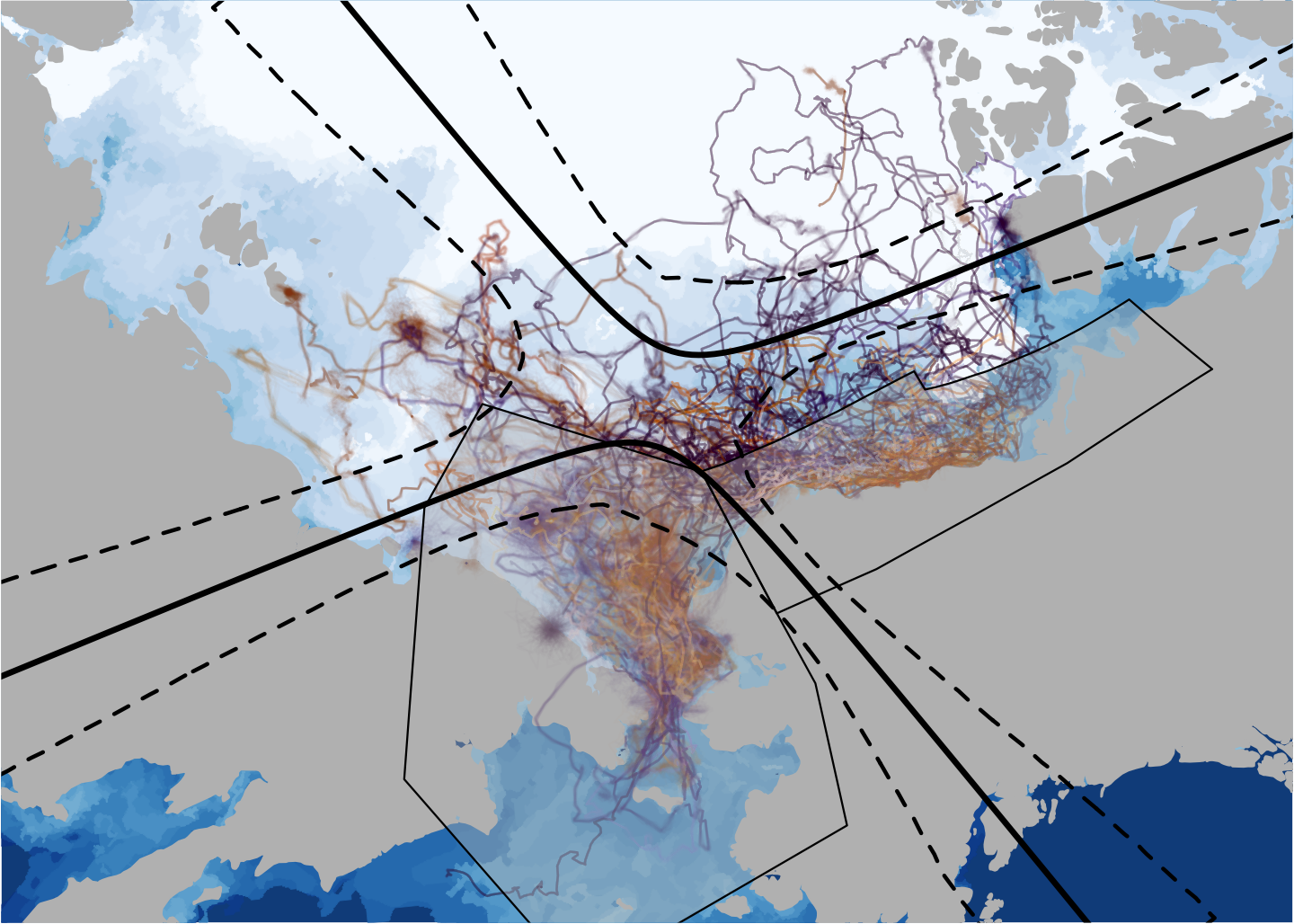
Using the two-stage approach, we fit the model to all observations made by USFWS and USGS from 2012–2016 (186 unique individuals). Table 3.6.1 gives the posterior medians and equal-tailed 95% credible intervals for each variance parameter, as well as relevant prior distributions and hyperpriors. Figure 3 shows the posterior mean of each grouped by the agency that tagged the individuals. Posterior means of the class indicator variables can be interpreted as the posterior probability that individual is a member of the Chukchi Sea sub-population.
| \Hline | posterior summary | prior | ||
| parameter | median | (2.5%, 97.5%) | density | |
| 272 | (267, 277) | |||
| 8600 | (8000, 9500) | |||
| 16.5 | (16.3, 16.6) | |||
| 93 | (89, 97) | |||
| see Figure 3 | ||||
| 69 | (28, 83) | |||
| 337 | (327, 349) | |||
To produce a meaningful spatial delineation of the two sub-populations from which our study animals were drawn, we use a derived quantity related to the inferred locations of the sub-population activity centers. If we consider the observation of a single new location, , and integrate across all arbitrary features, effectively removing the effect of the RSF, it can be shown that the posterior probability that is given by
For the case of an uninformative prior, , the contour corresponding to is defined by the points in the plane where the two normal densities are equal. It can be shown that these contours are the roots of quadratic polynomials in two dimensions. By computing the contour at each iteration in the MCMC algorithm, we can obtain draws from the posterior distribution, a summary of which provides wildlife managers with a way to delineate the boundary between the two sub-populations.
Figure 4 shows a map of the region encompassing the Chukchi and southern Beaufort seas. The solid black line corresponds to a central-measure summary of the posterior distribution of the derived spatial boundary, and the dashed lines show equal-tailed 95% pointwise credible intervals computed orthogonal to the solid line (more details are given in Supporting Information C). The portion of the inferred boundary most relevant in this application is in the bottom right quarter of the map and suggests at most a small shift from the currently accepted sub-population delineation, denoted by the large polygons with thin black lines (also shown in Figure 2). The discrepancy between the currently used sub-population boundary and the one we derive in this paper is likely due to a combination of factors including both the use of novel statistical methodology, and systematic changes to polar bear behavior as sub-populations respond to rapidly changing habitat conditions. We also note that a potentially informative landscape feature, ocean depth, has been included in past RSF analyses of polar bears but was not accounted for in this analysis. A goal of future statistical and ecological research is to develop methods that can account for both the sea ice boundary and landscape features like ocean depth.
3.6.2 Response to habitat characteristics
The posterior distribution of the parameters defining the “summer” season suggests that the feature , defined as the union of the interface between sea-ice and ocean and the continental coastlines, has the greatest impact on the behavior of polar bears between March 10 and December 3. While the end of the season aligns closely with prior expectations, there appears to be evidence in the data that polar bears show a preference for habitat near either coastlines or the edge of the sea ice more than two months earlier than expected. However, we note that because of the way telemetry devices were deployed, the posterior distribution for must be interpreted with caution. In particular, telemetry devices were affixed to polar bears each spring between mid-March and late-May opportunistically, with polar bears close to logistical bases located along the Arctic coast more likely to be tagged than polar bears far from the coastline (Wilson et al., 2014; Wilson et al., 2016). Additionally, the majority of units were affixed to females, as male polar bears require specialized radio transmitters. Thus, it is possible that the way in which data were gathered may be confounding our inference about the start of the “summer” season.
The posterior distribution for had a median value of approximately 90km, suggesting that polar bears prefer habitat within about 180km of the sea ice edge or coastline during the “summer” season on average. In comparison, Durner et al. (2004) concluded that polar bears selected habitat near the sea ice edge during July 24–May 30, with the strongest effect occurring during July 24–November 15 when polar bears showed a preference for habitat within about 100km. Durner et al. (2004) also showed that, from November 16–May 30 (approximately the period of maximum sea ice extent), polar bears continued to show a weakened preference for habitat near the sea ice interface, but at a larger range of distances. The relevant findings in Durner et al. (2009) were similar; polar bears showed a preference for habitat within approximately 200km of the sea ice edge. Durner et al. (2009) also found that, during the period of maximum sea ice extent, polar bears showed a preference for habitat within approximately 200km of coastlines. Thus, our conclusions about the timing and relevant spatial range of the effect of sea ice edge and coastline are consistent with those discussed in previous studies.
4 Discussion
Our novel approximation method based on the linearization of a potentially time-varying spatial feature, , reduces the computational burden of fitting models in the common RSF framework, allowing researchers increased flexibility in the types of RSFs they can specify in mechanistic models for movement. We demonstrated our approach in an application involving the movement of polar bears as they responded to seasonal shifts in sea ice during 2012–2016. Recently, there has been a significant increase in research focused on the so-called “greenwave” hypothesis (Aikens et al., 2017, e.g.,), which posits that herbivorous animals align their movement with bands of high-quality forage that shift throughout spring as different elevations and latitudes experience phenological changes. Our modeling approach represents a way to validate the hypothesis if information about the shape of the greenwave is known, or potentially estimate the location of the posited band of high quality forage based on the observed movement patterns of herbivores.
Several models for animal movement that seek to elucidate the complex relationship between individuals and their habitat have been proposed in the literature. Many recent models for movement are not explicitly framed in terms of RSFs, yet share important connections with our proposed methodology. A few important examples are Hanks et al. (2011); Hanks et al. (2015), and Buderman et al. (2018) who used the same multiple-imputation based two-stage approach to model individual responses to landscape features in a discrete-space framework. While Hanks et al. (2011); Hanks et al. (2015) required a third stage of analysis to obtain population-level inference, Buderman et al. (2018) used a hierarchical model construction similar to our approach that permits joint inference about individual and population-level parameters of interest, albeit at the cost of additional computation time. Additionally, Johnson et al. (2008) and Scharf et al. (2017) modeled individual-level movement using a continuous-space framework that is able to capture a tendency of individuals to “drift” toward particular landscape features. Importantly, while Hanks et al. (2011); Hanks et al. (2015), Scharf et al. (2017), and Buderman et al. (2018) allowed for time-varying responses to landscape features (analogous to the way we modeled a seasonal response of polar bears to the habitat described by ), none of these approaches explicitly accounted for dynamic landscape features that change in shape and location through time.
The linearization approximation methodology can also be extended to higher-dimensional spaces and features. For instance, in marine environments, RSFs based on two-dimensional features, such as isotherms, may be locally approximated using rank-deficient Gaussian distributions corresponding to infinite planes. One-dimensional features in three-dimensional spaces, such as wind or ocean currents, can also be approximated with improper distributions (see Supporting Information E for mathematical details). In practice, researchers will need to evaluate the appropriateness of a linearization approximation; however, in many cases, our methodology offers a way to include complex drivers of movement that might otherwise have been computationally inaccessible.
5 Supplementary Materials
Web Appendices A–E, which provide details related to the definition of the dynamic landscape feature (A), MCMC implementation (B), sub-population spatial boundary (C), simulation study (D), and extensions of the linearization approximation to higher dimensions (E) are available with this paper at the Biometrics website on Wiley Online Library.
Acknowledgments
The authors thank Franny Buderman, Perry Williams, and Christopher Peck for insight that improved the article. Any use of trade, firm, or product names is for descriptive purposes only and does not imply endorsement by the U.S. Government.
The views of the USFWS authors in this publication are solely those of the USFWS authors, and do not necessarily represent the views of the USFWS. This article has been peer-reviewed and approved by USGS under their Fundamental Science Practices policy (http://pubs.usgs.gov/circ/1367). This research was permitted under the Marine Mammal Protection Act and Endangered Species Act under U.S. Fish and Wildlife Service permits (MA046081, MA 690038) and followed protocols approved by Animal Care and Use Committees of the U.S. Fish and Wildlife Service and U.S. Geological Survey.
The authors acknowledge support for this research from NSF DMS 1614392 and USFWS G17AC00068.
References
- Aikens et al. (2017) Aikens, E. O., Kauffman, M. J., Merkle, J. A., Dwinnell, S. P., Fralick, G. L., and Monteith, K. L. (2017). The greenscape shapes surfing of resource waves in a large migratory herbivore. Ecology Letters 20, 741–750.
- Amstrup et al. (2005) Amstrup, S. C., Durner, G. M., Stirling, I., and McDonald, T. L. (2005). Allocating harvests among polar bear stocks in the Beaufort Sea. Arctic 53, 247–259.
- Atwood et al. (2016) Atwood, T. C., Peacock, E., McKinney, M. A., Lillie, K., Wilson, R. R., Douglas, D. C., Miller, S., and Terletzky, P. (2016). Rapid environmental change drives increased land use by an Arctic marine predator. PLoS ONE 11, e0155932.
- Brost et al. (2015) Brost, B. M., Hooten, M. B., Hanks, E. M., and Small, R. J. (2015). Animal movement constraints improve resource selection inference in the presence of telemetry error. Ecology 96, 2590–2597.
- Brost et al. (2016) Brost, B. M., Hooten, M. B., and Small, R. J. (2016). Leveraging constraints and biotelemetry data to pinpoint repetitively used spatial features. Ecology 98, 12–20.
- Buderman et al. (2018) Buderman, F. E., Hooten, M. B., Alldredge, M. W., Hanks, E. M., and Ivan, J. S. (2018). Time-varying predatory behavior is primary predictor of fine-scale movement of wildland-urban cougars. Movement Ecology 6,.
- Christ et al. (2008) Christ, A., Hoef, J. V., and Zimmerman, D. L. (2008). An animal movement model incorporating home range and habitat selection. Environmental and Ecological Statistics 15, 27–38.
- Crawford et al. (2012) Crawford, J. A., Frost, K. J., Quakenbush, L. T., and Whiting, A. (2012). Different habitat use strategies by subadult and adult ringed seals (Phoca hispida) in the Bering and Chukchi seas. Polar Biology 35, 241–255.
- Durner et al. (2004) Durner, G. M., Amstrup, S. C., Neilson, R., and McDonald, T. L. (2004). The use of sea ice habitat by female polar bears in the Beaufort Sea. U.S. Geological Survey, Alaska Science Center, Anchorage, Alaska. Outer Continental Shelf study, Minerals Management Service 2004–014 .
- Durner et al. (2009) Durner, G. M., Douglas, D. C., Nielson, R. M., Amstrup, S. C., McDonald, T. L., Stirling, I., Mauritzen, M., Born, E. W., Wiig, Ø., DeWeaver, E., Serreze, M. C., Belikov, S. E., Holland, M. M., Maslanik, J., Aars, J., Bailey, D. A., and Derocher, A. E. (2009). Predicting 21st-century polar bear habitat distribution from global climate models. Ecological Monographs 79, 25–58.
- Fetterer et al. (2010) Fetterer, F., Savoie, M., Helfrich, S., and Clemente-Colón, P. (2010). Multisensor analyzed aea ice extent - Northern hemisphere (MASIE-NH), version 1, updated daily. National Ice Center and National Snow and Ice Data Center 2008-2016, Boulder, Colorado USA. accessed August 13, 2017.
- Finley et al. (1983) Finley, K. J., Miller, G. W., Davis, R. A., and Koski, W. R. (1983). A Distinctive Large Breeding Population of Ringed Seals (Phoca hispida) Inhabiting the Baffin Bay Pack Ice. Arctic 36, 162–173.
- Frost et al. (2004) Frost, K. J., Lowry, L. F., Pendleton, G., and Nute, H. R. (2004). Factors affecting the observed densities of ringed seals, Phoca hispida, in the Alaskan Beaufort Sea. Arctic 57, 115–128.
- Hanks et al. (2015) Hanks, E. M., Hooten, M. B., and Alldredge, M. W. (2015). Continuous-time discrete-space models for animal movement. Annals of Applied Statistics 9, 145–165.
- Hanks et al. (2011) Hanks, E. M., Hooten, M. B., Johnson, D. S., and Sterling, J. T. (2011). Velocity-based movement modeling for individual and population level inference. PLoS ONE 6, e22795.
- Hjermann (2000) Hjermann, D. O. (2000). Analyzing habitat selection in animals without well defined home range. Ecology 81, 1462–1468.
- Hooten et al. (2017) Hooten, M. B., Johnson, D. S., McClintock, B. T., and Morales, J. M. (2017). Animal Movement: Statistical Models for Telemetry Data. Chapman and Hall/CRC, Boca Raton, Florida, USA.
- Johnson et al. (2006) Johnson, C. J., Nielsen, S. E., Merrill, E. H., McDonald, T. L., and Boyce, M. S. (2006). Resource selection functions based on use-availability data: theoretical motivation and evaluation methods. Journal of Wildlife Management 70, 347–357.
- Johnson et al. (2008) Johnson, D. S., London, J. M., Lea, M.-A., and Durban, J. W. (2008). Continuous-time correlated random walk model for animal telemetry data. Ecology 89, 1208–1215.
- Johnson et al. (2008) Johnson, D. S., Thomas, D. L., Ver Hoef, J. M., and Christ, A. (2008). A general framework for the analysis of animal resource selection from telemetry data. Biometrics 64, 968–976.
- Kelly et al. (2010) Kelly, B. P., Bengtson, P. L., Boveng, P. L., Cameron, M. F., Dahle, S. P., Jansen, J. K., Logerwell, E. A., Overland, J. E., Sabine, C. L., Waring, G. T., and Wilder, J. M. (2010). Status review of the ringed seal (Phoca hispida). U.S. Dep. Commer., NOAA Tech. Memo. NMFS-AFSC-212 pages 1–250.
- Lele and Keim (2006) Lele, S. R. and Keim, J. L. (2006). Weighted distributions and estimation of resource selection probability functions. Ecology 87, 3021–3028.
- Manly et al. (2002) Manly, B. F. J., Mcdonald, L. L., and Thomas, D. L. (2002). Resource Selection by Animals: Statistical Design and Analysis for Field Studies. Springer, second edition.
- Niu et al. (2016) Niu, M., Blackwell, P. G., and Skarin, A. (2016). Modeling interdependent animal movement in continuous time. Biometrics 72, 315–324.
- Northrup et al. (2013) Northrup, J. M., Hooten, M. B., Anderson, C. R. J., and Wittemyer, G. (2013). Practical guidance on characterizing availabilty in resource selection functions under a use-availability design. Ecology 94, 1456–1463.
- Obbard et al. (2010) Obbard, M. E., Thiemann, G. W., Peacock, E., and Debruyn, T. D. (2010). Proceedings of the 15th working meeting of the IUCN/SCC polar bear specialist group, 29 June - 3 July 2009, Copenhagen, Denmark. In IUCN, volume vii, page 235.
- Rode et al. (2014) Rode, K. D., Regehr, E. V., Douglas, D. C., Durner, G. M., Derocher, A. E., Thiemann, G. W., and Budge, S. M. (2014). Variation in the response of an Arctic top predator experiencing habitat loss: Feeding and reproductive ecology of two polar bear populations. Global Change Biology 20, 76–88.
- Rode et al. (2015) Rode, K. D., Wilson, R. R., Regehr, E. V., Martin, M. S., Douglas, D. C., and Olson, J. W. (2015). Increased land use by Chukchi Sea polar bears in relation to changing sea ice conditions. PLoS ONE 10, e0142213.
- Scharf et al. (2016) Scharf, H. R., Hooten, M. B., Fosdick, B. K., Johnson, D. S., London, J. M., and Durban, J. W. (2016). Dynamic social networks based on movement. Annals of Applied Statistics 10, 2182–2202.
- Scharf et al. (2017) Scharf, H. R., Hooten, M. B., and Johnson, D. S. (2017). Imputation approaches for animal movement modeling. Journal of Agricultural, Biological, and Environmental Statistics 22, 335–352.
- Scharf et al. (2018) Scharf, H. R., Hooten, M. B., Johnson, D. S., and Durban, J. W. (2018). Process convolution approaches for modelling interacting trajectories. Environmetrics 29, e2487.
- Tracey et al. (2005) Tracey, J. A., Zhu, J., and Crooks, K. R. (2005). A set of nonlinear regression models for animal movement in response to a single landscape feature. Journal of Agricultural, Biological, and Environmental Statistics 10, 1–18.
- U.S. Fish and Wildlife (2016) U.S. Fish and Wildlife (2016). Polar bear (Ursus maritimus) conservation management plan, final. U.S. Fish and Wildlife, Region 7, Anchorage, Alaska pages 1–104.
- Ware et al. (2017) Ware, J. V., Rode, K. D., Bromaghin, J. F., Douglas, D. C., Wilson, R. R., Regehr, E. V., Amstrup, S. C., Durner, G. M., Pagano, A. M., Olson, J. W., Robbins, C. T., and Jansen, H. T. (2017). Habitat degradation affects the summer activity of polar bears. Oecologia 184, 87–99.
- Warton and Shepherd (2010) Warton, D. I. and Shepherd, L. C. (2010). Poisson point process models solve the “pseudo-absence problem” for presence-only data in ecology. Annals of Applied Statistics 4, 1383–1402.
- Wiig et al. (1999) Wiig, Ø., Derocher, A. E., and Belikov, S. E. (1999). Ringed seal (Phoca hispida) breeding in the drifting ice of the Barents Sea. Marine Mammal Science 15, 595–598.
- Wilson et al. (2014) Wilson, R. R., Horne, J. S., Rode, K. D., Regehr, E. V., and Durner, G. M. (2014). Identifying polar bear resource selection patterns to inform offshore development in a dynamic and changing Arctic. Ecosphere 5, 136.
- Wilson et al. (2016) Wilson, R. R., Regehr, E. V., Rode, K. D., and St Martin, M. (2016). Invariant polar bear habitat selection during a period of sea ice loss. Proceedings of the Royal Society B: Biological Sciences 283, 20160380.