Does data interpolation contradict statistical optimality?

In this paper, we exhibit estimators that interpolate the data, yet achieve optimal rates of convergence for the problems of nonparametric regression and prediction with square loss. This curious observation goes against the usual (or, folklore?) intuition that a good statistical procedure should forego the exact fit to data in favor of a more smooth representation. The family of estimators we consider do exhibit a bias-variance trade-off with a tuning parameter, yet this “regularization” co-exists in harmony with data interpolation.

Motivation for this work is the recent focus within the machine learning community on the out-of-sample performance of neural networks. These flexible models are typically trained to fit the data exactly (either in their sign or in the actual value), yet they predict well on unseen data. The conundrum has served both as a source of excitement about the “magical” properties of neural networks, as well as a call for the development of novel statistical techniques to resolve it.

The aim of this short note is to show that not only can interpolation be a good statistical procedure, but it can even be optimal in a minimax sense. To the best of our knowledge, such optimality has not been exhibited before.

Let $(X,Y)$ be a random pair on ${\mathbb{R}}^{d}\times{\mathbb{R}}$ with distribution $P_{XY}$, and let $f(x)=\mathbb{E}[Y|X=x]$ be the regression function. A goal of nonparametric estimation is to construct an estimate $f_{n}$ of $f$, given a sample $(X_{1},Y_{1}),\ldots,(X_{n},Y_{n})$ drawn independently from $P_{XY}$. A classical approach to this problem is kernel smoothing. In particular, the Nadaraya-Watson estimator (Nadaraya, 1964; Watson, 1964) is defined as

where $K:{\mathbb{R}}^{d}\to{\mathbb{R}}$ is a kernel function and $h>0$ is a bandwidth and we assume that the denominator does not vanish. Appropriate choices of $K$ and $h$ lead to optimal rates of estimation, under various assumptions, and we refer the reader to (Tsybakov, 2009) and references therein.

We consider singular kernels that approach infinity when their argument tends to zero. It has been observed, at least since (Shepard, 1968), that the resulting function in (1) interpolates the data. We will focus on the particular kernel

for some $a>0$. Here, $\left\|\cdot\right\|$ denotes the Euclidean norm. Our results can be extended to other related singular kernels, for example, to

where $[c]_{+}=\max\{c,0\}$, and

considered in (Lancaster and Salkauskas, 1981; Katkovnik, 1985). Also, $\left\|\cdot\right\|$ can be any norm on ${\mathbb{R}}^{d}$, not necessarily the Euclidean norm.

Our main result, stated precisely in the next section and proved in Section 4, establishes that

whenever the regression function $f$ belongs to a Hölder class with parameter $\beta\in(0,2]$, and under additional assumptions stated below. Here $C$ is a constant that does not depend on $n$ and $P_{X}$ is the marginal distribution of $X$. The rate $n^{-\frac{2\beta}{2\beta+d}}$ is the classical minimax optimal rate for these classes.

Our result also yields a curious conclusion for the problem of prediction with square loss. Observe that excess loss—an object studied in Statistical Learning Theory—with respect to a Hölder class $\Sigma(\beta,L)$, formally defined below, can be written as

under the assumption that the model is well-specified (that is, the regression function is in the class). We remark that the estimator $f_{n}$ is improper, in the sense that it does not itself belong to the Hölder class (its smoothness depends on $h$ and, hence, on $n$). In conclusion, despite the fact that $f_{n}$ is improper and fits the data exactly, it attains optimal rates for excess loss. We refer the reader to (Rakhlin et al., 2017) for further discussion of optimal rates in nonparametric estimation and statistical learning.

We start with a definition.

We assume the following.

• (A1)

  For any $x\in{\mathbb{R}}^{d}$, the expectation $\mathbb{E}[Y|X=x]=f(x)$ exists and $\mathbb{E}[\xi^{2}|X=x]\leq\sigma^{2}_{\xi}<\infty$, where $\xi=Y-\mathbb{E}[Y|X]=Y-f(X)$.

• (A2)

  The marginal density $p(\cdot)$ of $X$ exists and satisfies $0<p_{\min}\leq p(x)\leq p_{\max}$ for all $x$ on its support.

The Nadaraya-Watson estimator for a singular kernel $K$ is defined as

The two main results for this estimator are now stated.

The pointwise mean squared error (MSE) bounds of Theorems 1 and 2 immediately imply the integrated MSE with respect to the marginal distribution of $X$:

assuming that $f$ is bounded on the support of the marginal density $p$.

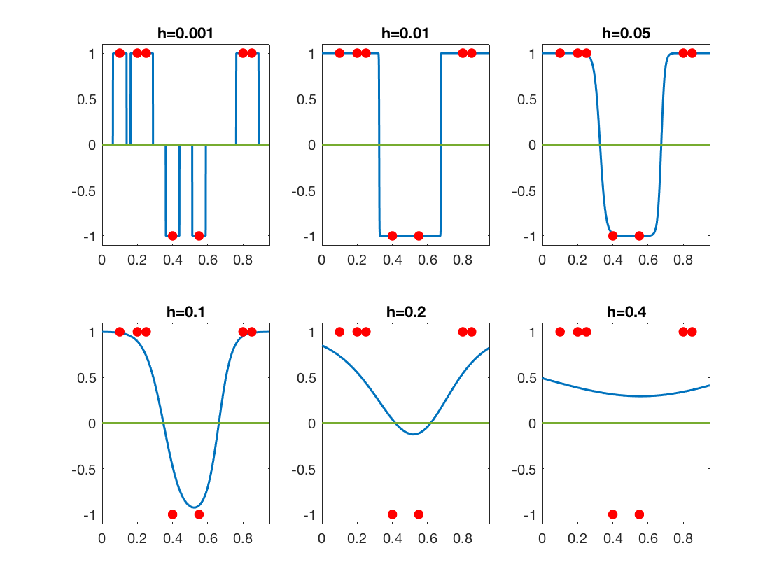
The figures below show interpolations with kernels (2) and (3). While both achieve optimal rates of convergence in this simple one-dimensional problem, the latter kernel appears to be less irregular. Indeed, unlike (2), kernels (3) and (4) produce continuous functions.

We now compare Figures 1 and 2 to those with a non-singular kernel. We remark that choices of bandwidth $h$ differ depending on the kernel, and direct comparisons for the same value across kernels might not be meaningful.

Figure 5 below shows a comparison between the interpolating kernel 3 and the Gaussian kernel for binary-valued data. We observe the more global effect that each point has on the behavior of the solution with the Gaussian kernel, in comparison to the singular kernel. Understanding properties of the plug-in classifier $\text{sign}(f_{n})$ under various margin conditions appears to be an interesting direction of further research.

Without loss of generality, consider the problem of estimating $f(x_{0})$ at $x_{0}=0$, assuming it is in the support of $p$ and $|f(x_{0})|<\infty$.

Consider the event

and observe that

for a constant $C>0$ that does not depend on $n$. On the event $\bar{\mathcal{E}}$, we have $f_{n}(0)=0$ and thus the contribution to expected risk is at most $M_{\mathcal{E}}=f(0)^{2}\exp\left\{-Cp_{\min}nh^{d}\right\},$ a lower-order term compared to the remaining calculations.

On the event $\mathcal{E}$, the estimator $f_{n}(0)$ is equal to

(modulo an event of zero probability with respect to the joint distribution of $X_{1},\ldots,X_{n}$), where

Set $\xi_{i}=Y_{i}-f(X_{i})$. Let $\mathbb{E}_{Y}$ denote the expectation with respect to $Y_{1},\ldots,Y_{n}$, conditional on $X_{1},\ldots,X_{n}$. We have the following “bias-variance” decomposition

It holds that, on the event $\mathcal{E}$,

and, hence, the variance term is

where

On the other hand, the bias¹¹ 1 To be precise, this term includes variance due to random $X$, as will be clear from Lemma 3. is

The following lemmas control each of the above expressions under various assumptions on $f$ and the marginal density $p$. We will denote by $C$ positive constants that can vary from line to line.

We presented a proof of concept: an interpolating rule can achieve optimal rates for the problems of nonparametric estimation and prediction with square loss. Our proof technique extends to other kernels where the indicator over the unit Euclidean ball in (2) is replaced with a function that dominates an appropriately scaled indicator. The analysis also works for non-singular kernels under the assumption of square integrability (required only in Eq. (12)).

While each pair $(X_{i},Y_{i})$ is fit exactly by the proposed estimator, the influence of the datapoint is local. In aggregate, however, the function $f_{n}$ is being “pulled” towards the true regression function $f$. Whether a similar phenomenon occurs in other interpolating rules—such as overparametrized neural networks—requires further investigation.

References

• Belkin et al. (2018) Mikhail Belkin, Daniel Hsu, and Partha Mitra. Overfitting or perfect fitting? risk bounds for classification and regression rules that interpolate. arXiv preprint arXiv:1806.05161, 2018.
• Chaudhuri and Dasgupta (2014) Kamalika Chaudhuri and Sanjoy Dasgupta. Rates of convergence for nearest neighbor classification. In Advances in Neural Information Processing Systems, pages 3437–3445, 2014.
• Cover and Hart (1967) Thomas Cover and Peter Hart. Nearest neighbor pattern classification. IEEE transactions on information theory, 13(1):21–27, 1967.
• Devroye et al. (1996) Luc Devroye, László Györfi, and Gábor Lugosi. A probabilistic theory of pattern recognition. Springer, 1996.
• Devroye et al. (1998) Luc Devroye, Laszlo Györfi, and Adam Krzyżak. The Hilbert kernel regression estimate. Journal of Multivariate Analysis, 65(2):209–227, 1998.
• Katkovnik (1985) V Katkovnik. Nonparametric identification and smoothing of data (Local approximation methods). Nauka, Moscow, 1985.
• Lancaster and Salkauskas (1981) Peter Lancaster and Kes Salkauskas. Surfaces generated by moving least squares methods. Mathematics of computation, 37(155):141–158, 1981.
• Nadaraya (1964) Elizbar A Nadaraya. On estimating regression. Theory of Probability & Its Applications, 9(1):141–142, 1964.
• Rakhlin et al. (2017) Alexander Rakhlin, Karthik Sridharan, and Alexandre B Tsybakov. Empirical entropy, minimax regret and minimax risk. Bernoulli, 23(2):789–824, 2017.
• Shepard (1968) Donald Shepard. A two-dimensional interpolation function for irregularly-spaced data. In Proceedings of the 1968 23rd ACM national conference, pages 517–524. ACM, 1968.
• Tsybakov (2009) Alexandre B Tsybakov. Introduction to nonparametric estimation. Springer Series in Statistics. Springer, New York, 2009.
• Watson (1964) Geoffrey S Watson. Smooth regression analysis. Sankhyā: The Indian Journal of Statistics, Series A, pages 359–372, 1964.