Optimized Video Streaming over Cloud: A Stall-Quality Trade-off
Abstract
As video-streaming services have expanded and improved, cloud-based video has evolved into a necessary feature of any successful business for reaching internal and external audiences. In this paper, video streaming over distributed storage is considered where the video segments are encoded using an erasure code for better reliability. There are multiple parallel streams between each server and the edge router. For each client request, we need to determine the subset of servers to get the data, as well as one of the parallel stream from each chosen server. In order to have this scheduling, this paper proposes a two-stage probabilistic scheduling. The selection of video quality is also chosen with a certain probability distribution. With these parameters, the playback time of video segments is determined by characterizing the download time of each coded chunk for each video segment. Using the playback times, a bound on the moment generating function of the stall duration is used to bound the mean stall duration. Based on this, we formulate an optimization problem to jointly optimize the convex combination of mean stall duration and average video quality for all requests, where the two-stage probabilistic scheduling, probabilistic video quality selection, bandwidth split among parallel streams, and auxiliary bound parameters can be chosen. This non-convex problem is solved using an efficient iterative algorithm. Evaluation results show significant improvement in QoE metrics for cloud-based video as compared to the considered baselines.
Index Terms:
Video Streaming over Cloud, Erasure Codes, Mean Stall Duration, Video Quality, Two-stage probabilistic scheduling.I Introduction
Cloud computing has changed the way many Internet services are provided and operated. Video-on-Demand (VoD) providers are increasingly moving their streaming services, data storage, and encoding software to cloud service providers [1, 2]. With the annual growth of global video streaming at a rate of 18.3% [3], cloud-based video has become an imperative feature of any successful business. For example, IBM estimates cloud-based video will be a $105 billion market opportunity by 2019 [4]. In this paper, we will give a novel approach to an optimized cloud-based-video streaming.
Since the computing has been growing exponentially [5], the computation of decoding will not limit the latencies in delay sensitive video streaming and the networking latency will govern the system designs. The key advantage of erasure coding is that it reduces storage cost while providing similar reliability as replicated systems [6, 7], and thus has now been widely adopted by companies like Facebook [8], Microsoft [9], and Google [10]. Further, we note that replication is a special case of erasure coding. Thus, the proposed research using erasure-coded content on the servers can also be used when the content is replicated on the servers.
In cloud-based-video, the users are connected to an edge router, which fetch the contents from the distributed storage servers (as depicted in Fig. 1). There are multiple parallel streams (PSs) between a server and the edge router which help in getting multiple streams simultaneously. We assume that the connection between users and edge router is not limited. Unlike the case of file download, the later video-chunks do not have to be downloaded as fast as possible to improve the quality-of-experience (QoE) and thus multiple parallel streams help achieve better QoE. The key QoE metrics for video streaming are the duration of stalls at the clients and the streamed average video quality. Every viewer can relate the QoE for watching videos to the stall duration and is thus one of the key focus in the studied streaming algorithms [11, 12]. The average quality of the streamed video is an important QoE metric.
The key challenge in quantification of stall duration is the choice of scheduling strategy to choose the storage servers for each request, as well as the parallel stream from the chosen servers. For a single video-chunk and single quality videos, the problem is equivalent to minimizing the download latency. This problem is an open problem, since the optimal strategy of choosing these servers (when file is erasure coded with parameters ) would need a Markov approach similar to that in [13] which suffers from a state explosion problem. Further, the choice of video quality makes the problem challenging since the choice of video quality would depend on the current queue states. The authors of [14, 15] proposed a probabilistic scheduling method for file scheduling, where each possibility of servers is chosen with certain probability that can be optimized. In this paper, we extend this scheduling to a two-stage probabilistic scheduling which chooses servers and one of the parallel streams from each of these servers. Further, the choice of video quality is chosen independent of the scheduling and is chosen by a discrete probabilistic distribution. Thus, the proposed scheduling and quality assignment do not account for the current queue state making the approach manageable for analysis.
The data chunk transfer time in practical systems follows a shifted exponential distribution [15, 16] which motivates the choice that the service time distribution for each video server is a shifted exponential distribution. Further, the request arrival rates for each video is assumed to be Poisson. The video segments are encoded using an erasure code and the coded segments are placed on different servers. When a video is requested, the segments need to be requested from out of servers as well as one of the parallel streams from each of the servers. Using the two-stage probabilistic scheduling and probabilistic quality assignment, the random variables corresponding to the times for download of different video segments from each server are characterized. By using ordered statistics over the parallel streams (one from each of the chosen servers), the random variables corresponding to the playback time of each video segment are then calculated. These are then used to find a bound on the mean stall duration. Moment generating functions of the ordered statistics of different random variables are used in the bound. We note that the problem of finding latency for file download is very different from the video stall duration for streaming. This is because the stall duration accounts for download time of each video segment rather than only the download time of the last video segment. Further, the download time of segments are correlated since the download of chunks from a server are in sequence and the playback time of a video segment are dependent on the playback time of the last segment and the download time of the current segment. Taking these dependencies into account, this paper characterizes the bound on the mean stall duration.
A convex combination of mean stall duration and average video quality is optimized over the choice of two-stage probabilistic scheduling, video quality assignment probability, bandwidth allocation among different streams, and the auxiliary variables in the bounds. Changing the convex combination parameter gives a tradeoff between the mean stall duration and the average video quality. An efficient algorithm is proposed to solve this non-convex problem. The proposed algorithm performs an alternating optimization over the different parameters, where each sub-problem is shown to have convex constraints and thus can be efficiently solved using iNner cOnVex Approximation (NOVA) algorithm proposed in [17]. The proposed algorithm is shown to converge to a local optimal. Evaluation results demonstrate significant improvement of QoE metrics as compared to the considered baselines. The key contributions of our paper are summarized as follows.
- •
This paper proposes a two-stage probabilistic scheduling for the choice of servers and the parallel streams. Further, the video quality is chosen using a discrete probability distribution.
- •
Two-stage probabilistic scheduling and probabilistic quality assignment are used to find the distribution of the (random) download time of a chunk of each video segment from a parallel stream. Using ordered statistics, the random variable corresponding to the playback time of each video segment is characterized. This is further used to give bounds on the mean stall duration.
- •
The QoE metrics of mean stall duration and average video quality are used to formulate an optimization problem over the two-stage probabilistic scheduling access policy, probabilistic quality assignment, the bandwidth allocation weights among the different streams, and the auxiliary bound parameters which are related to the moment generating function. Efficient iterative solutions are provided for these optimization problems.
- •
The experimental results validate our theoretical analysis and demonstrate the efficacy of our proposed algorithm. Further, numerical results show that the proposed algorithms converge within a few iterations. Further, the QoE metrics are shown to have significant improvement as compared to the considered baselines. Even for the minimum stall point, the proposed algorithm gets better quality than the lowest quality. Further, the tradeoff between stalls and quality can be used by the service provider to effectively find an operating point.
The remainder of this paper is organized as follows. Section II provides related work for this paper. In Section III, we describe the system model used in the paper with a description of video streaming over cloud storage. Section IV derives expressions for the download and play times of the chunks which are used in Section V to find an upper bound on the mean stall duration. Section VI formulates the QoE optimization problem as a weighted combination of the two QoE metrics and proposes the iterative algorithmic solution of this problem. Numerical results are provided in Section VII. Section VIII concludes the paper.
II Related Work
Latency in Erasure-coded Storage: To our best knowledge, however, while latency in erasure coded storage systems has been widely studied, quantifying exact latency for erasure-coded storage system in data-center network is an open problem. Recently, there has been a number of attempts at finding latency bounds for an erasure-coded storage system [18, 19, 13, 14, 15, 16]. The key scheduling approaches include block-one-scheduling policy that only allows the request at the head of the buffer to move forward [18], fork-join queue [20, 19] to request data from all server and wait for the first to finish, and the probabilistic scheduling [14, 15] that allows choice of every possible subset of nodes with certain probability. Mean latency and tail latency have been characterized in [14, 15] and [21, 22], respectively, for a system with multiple files using probabilistic scheduling. The probabilistic scheduling has also been shown to be optimal for tail latency index when the file sizes are heavy-tailed [23]. This paper considers video streaming rather than file downloading. The metrics for video streaming does not only account for the end of the download of the video but also of the download of each of the segment. Thus, the analysis for the content download cannot be extended to the video streaming directly and the analysis approach in this paper is very different from the prior works in the area.
Video Streaming over Cloud: Servicing Video on Demand and Live TV Content from cloud servers have been studied widely [24, 25, 26, 27, 28]. The placement of content and resource optimization over the cloud servers have been considered. To the best of our knowledge, reliability of content over the cloud servers have not been considered for video streaming applications. In the presence of erasure-coding, there are novel challenges to characterize and optimize the QoE metrics at the end user. Adaptive streaming algorithms have also been considered for video streaming [29, 30], which are beyond the scope of this paper and are left for future work.
Recently, the authors of [31] considered video-streaming over cloud. However, the videos were a single quality and the quality optimization was not accounted. Further, [31] considered single stream between each storage server and edge node and thus two-stage probabilistic scheduling was not needed. Thus, the analysis and the problem formulation in this work is different from that in [31].
III System Model

We consider a distributed storage system consisting of heterogeneous servers (also called storage nodes), denoted by . Each server can be split into virtual outgoing parallel streams (queues) to the edge router, where the server bandwidth is split among all parallel streams (PSs). This is depicted in Fig. 1. The reason of having PSs is to serve video files simultaneously from a server thus helping one file not to have files wait for the previous long video files. This is a key difference for video streaming as compared to file download since the deadline for the later video chunks are late thus motivating prioritizing earlier chunks. This parallelization helps download multiple files in parallel which also delays the finishing of download of the last chunks of multiple requests. Multiple users are connected to edge-router, where we assume that the connection between user and edge router is infinite and thus only consider the links from the server to the edge router. Thus, we can consider edge router as an aggregation of multiple users. Let be a set of non-negative weights representing the split of bandwidth at server on the PSs. The weights satisfy . The sum of weights at all PSs can be smaller than , representing that the bandwidth may not be completely utilized. By optimizing , the server bandwidth can be efficiently split among different PSs. Optimizing these weights help avoid bandwidth under-utilization and congestion, for example, assigning larger bandwidth to heavy workload PSs can help reduce mean stall duration.
Each video file , where is divided into equal segments, each of length seconds. We assume that each video file is encoded to different qualities, i.e., , where are the number of possible choices for the quality level. The segments of video file at quality are denoted as . Then, each segment for and is partitioned into fixed-size chunks and then encoded using an Maximum Distance Separable (MDS) erasure code to generate distinct chunks for each segment . These coded chunks are denoted as . The encoding setup is illustrated in Figure 2. The encoded chunks for all quality levels are stored on the disks of distinct storage nodes. The storage nodes chosen for quality level are represented by a set , such that and . Each server stores all the chunks for all and for some . In other words, servers store the entire content, where a server stores coded chunk for all the video-chunks for some or does not store any chunk. We will use a probabilistic quality assignment strategy, where a chunk of quality of size is requested with probability for all . We further assume all the chunks of the video are fetched at the same quality level. Note that indicates that the video file is replicated times.
In order to serve the incoming request at the edge router, the video can be reconstructed from the video chunks from any subset of -out-of- servers. Further, we need to assign one of the PSs for each server that is selected. We assume that files at each PS are served in order of the request in a first-in-first-out (FIFO) policy. Further, the different video chunks in a video are processed in order. In order to select the different PSs for video and quality , the request goes to a set , with and for every and in , . Here, the choice of represents the server to choose and represents the PS selected. From each choice , all chunks for all and the value of corresponding to that placed on server are requested from PS . The choice of optimal scheduling strategy, or set is an open problem. In this paper, we extend the probabilistic scheduling proposed in [14, 15] to two-stage probabilistic scheduling. The two-stage probabilistic scheduling chooses every possible subset of -out-of- nodes with certain probability, and for every chosen node , chooses -out-of- PSs with certain probability. Let is the probability of requesting file from the PS that belongs to server for quality level . Thus, is given by
| (1) |
where is the probability of choosing server and is the probability of choosing PS at server . Following [14, 15], it can be seen that the two-stage probabilistic scheduling gives feasible probabilities for choosing -out-of nodes and one-out-of- PSs if and only if there exists conditional probabilities and satisfying
| (2) |
and
| (3) |
We now describe a queuing model of the distributed storage system. We assume that the arrival of requests at the edge router for each video form an independent Poisson process with a known rate . Using the two stage probabilistic scheduling and the quality assignment probability distribution, the arrival of file requests at PS at node forms a Poisson Process with rate which is the superposition of Poisson processes each with rate . We assume that the chunk service time for each coded chunk at PS of server , , follows a shifted exponential distribution as has been demonstrated in realistic systems [15, 16] and is given by the probability distribution function , which is
| (4) |
We note that exponential distribution is a special case with . Let be the moment generating function of whose quality is . Then, is given as
| (5) |
Note that the value of increases in proportion to the chunk size, and the value of decreases in proportion to the chunk size in the shifted-exponential service time distribution. Further, the rate is proportional to the assigned bandwidth . More formally, the parameters and are given as
| (6) |
where and are constant service time parameters when and the entire bandwidth is allocated to one PS. Since mainly represents the read time and other processing times, we assume that all PSs have the same value of .
We note that the arrival rates are given in terms of the video files, and the service rate above is provided in terms of the coded chunks at each server. The client plays the video segment after all the chunks for the segment have been downloaded and the previous segment has been played. We also assume that there is a start-up delay of (in seconds) for the video which is the duration in which the content can be buffered but not played. This paper will characterize the mean stall duration using two-stage probabilistic scheduling and probabilistic quality assignment.
IV Download and Play Times of the Chunks
In order to understand the stall duration, we need to see the download time of different coded chunks and the play time of the different segments of the video.
IV-A Download Times of the Chunks from each Server
In this subsection, we will quantify the download time of chunk for video file from server which has chunks for all . The download of consists of two components - the waiting time of the video files in the queue of the PS before file request and the service time of all chunks of video file up to the chunk. Let be the random variable corresponding to the waiting time of all the video files in queue of PS at server before file request and be the (random) service time of coded chunk for file with quality from PS at server . Then, the (random) download time for coded chunk for file at PS at server , , is given as
| (7) |
We will now find the distribution of . We note that this is the waiting time for the video files whose arrival rate is given as . In order to find the waiting time, we would need to find the service time statistics of the video files. Note that gives the service time distribution of only a chunk and not of the video files.
Video file of quality consists of coded chunks at PS at server (). The total service time for video file with quality at PS at server if requested from server , , is given as
| (8) |
The service time of the video files is given as
| (9) |
since the service time is when file is requested at quality from PS from server . Let be the Laplace-Stieltjes Transform of .
Lemma 1.
The Laplace-Stieltjes Transform of , is given as
| (10) |
Proof.
| (11) |
∎
Corollary 1.
The moment generating function for the service time of video files when requested from server and PS , , is given as
| (12) |
for any , and .
Proof.
This corollary follows from (10) by setting . ∎
The server utilization for the video files at PS of server is given as . Since , using Lemma 1, we have
| (13) |
Having characterized the service time distribution of the video files via a Laplace-Stieltjes Transform , the Laplace-Stieltjes Transform of the waiting time can be characterized using Pollaczek-Khinchine formula for M/G/1 queues [32], since the request pattern is Poisson and the service time is general distributed. Thus, the Laplace-Stieltjes Transform of the waiting time is given as
| (14) |
By characterizing the Laplace-Stieltjes Transform of the waiting time and knowing the distribution of , the Laplace-Stieltjes Transform of the download time is given as
| (15) |
We note that the expression above holds only in the range of when and . Further, the server utilization must be less than . The overall download time of all the chunks for the segment at the client, , is given by
| (16) |
IV-B Play Time of Each Video Segment
Let be the time at which the segment is played (started) at the client. The startup delay of the video is . Then, the first segment can be played at the maximum of the time the first segment can be downloaded and the startup delay. Thus,
| (17) |
For , the play time of segment of file is given by the maximum of the time it takes to download the segment and the time at which the previous segment is played plus the time to play a segment ( seconds). Thus, the play time of segment of file , can be expressed as
| (18) |
Equation (18) gives a recursive equation, which can yield
| (19) | |||||
where
| (20) |
Since from (16), can be written as
| (21) |
We next give the moment generating function of that will be used in the calculations of the mean stall duration in the next section.
Lemma 2.
The moment generating function for , is given as
| (22) |
where
| (23) |
Proof.
Ideally, the last segment should have started played by time . The difference between and gives the stall duration. We note that is not the download time of the last segment, but the play time of the last segment and accounts for the download of all the segments. This is a key difference as compared to the file download since the download time of each segment of the video has to be accounted for computing stall duration. Thus, the stall duration for the request of video file of quality , i.e., , is given as
| (24) |
In the next section, we will use this stall time to determine the bound on the mean stall duration of the streamed video.
V Mean Stall Duration
In this section, we will provide a bound on the mean stall duration for a file . We will find the bound by two-stage probabilistic scheduling and since this scheduling is one feasible strategy, the obtained bound is an upper bound to the optimal strategy. Using (24), the expected stall time for file is given as follows
| (25) | |||||
Exact evaluation for the play time of segment is hard due to the dependencies between random variables for different values of , , , and , where and . Hence, we derive an upper-bound on the playtime of the segment as follows. Using Jensen’s inequality [33], we have for ,
| (26) |
Thus, finding an upper bound on the moment generating function for can lead to an upper bound on the mean stall duration. Thus, we will now bound the moment generating function for .
| (27) | |||||
| (28) | |||||
| (29) |
| (30) | |||||
| (31) | |||||
| (32) | |||||
| (33) |
where (a) follows from (21), (b) follows by upper bounding by , (c) follows by two-stage probabilistic scheduling where , and . We note that the only inequality here is for replacing the maximum by the sum. Since this term will be inside the logarithm for the mean stall latency, the gap between the term and its bound becomes additive rather than multiplicative.
To use the bound (33), needs to be bounded too. Thus, an upper bound on is calculated as follows.
| (34) |
where (d) follows by bounding the maximum by the sum, (e) follows from (22), and (f) follows by substituting .
| (35) |
Further, substituting the bounds (34) and (35) in (25), the mean stall duration is bounded as follows.
| (36) | |||||
where . Let
, which is the inner summation in (36). can be simplified using the geometric series formula to obtain
Theorem 1.
The mean stall duration time for file streamed with quality is bounded by
| (39) |
for any , ,
.
Note that Theorem above holds only in the range of when which reduces to
,
and . Further, the server utilization must be less than for stability of the system.
VI Optimization Problem Formulation and Proposed Algorithm
VI-A Problem Formulation
Let , , , , and
. We wish to minimize the two proposed QoE metrics over the choice of two-stage probabilistic scheduling parameters, bandwidth allocation, probability of the quality of the streamed video and auxiliary variables. Since this is a multi-objective optimization, the objective can be modeled as a convex combination of the two QoE metrics.
Let be the total arrival rate of file . Then, is the ratio of video requests. The first objective is the minimization of the mean stall duration, averaged over all the file requests, and is given as . The second objective is maximizing the streamed quality of all video requests, averaged over all the file requests, and is given as . Using the expressions for the mean stall duration in Section V and the average streamed quality, optimization of a convex combination of the two QoE metrics can be formulated as follows.
| (41) | |||
| (42) | |||
| (43) |
| (44) | |||
| (45) | |||
| (46) | |||
| (47) | |||
| (48) | |||
| (49) | |||
| (50) | |||
| (51) | |||
| (52) |
Here, is a trade-off factor that determines the relative significance of the mean stall duration and the average streamed quality in the minimization problem. Varying to , the solution for (40) spans the solutions that maximize the video quality to those minimizing the mean stall duration. The equations (37), (38), (5), (12), (13), (1), and (6) give the terms in the objective function. The constraint (41) indicates that the load intensity of server is less than . Equation (42) gives the aggregate arrival rate for each node. Constraints (43), (44), and (45) guarantee that the two-stage scheduling probabilities are feasible. Constraint (46) guarantees that the quality assignment probabilities are feasible and (48) is for bandwidth splitting among different streams. Constraints (49), (50), and (51) ensure that and the moment generating function given in (23) exist. In the next subsection, we will describe the proposed algorithm for this optimization problem.
VI-B Proposed Algorithm
The mean stall duration optimization problem given in (40)-(52) is optimized over five set of variables: server scheduling probabilities , PS selection probabilities , auxiliary parameters , video quality parameters , and bandwidth allocation weights . We first note that the problem is non-convex in all the parameters jointly, which can be easily seen in the terms which are product of the different variables. Since the problem is non-convex, we propose an iterative algorithm to solve the problem. The proposed algorithm divides the problem into five sub-problems that optimize one variable while fixing the remaining four. The five sub-problems are labeled as (i) Server Access Optimization: optimizes , for given , , and , (ii) PS Selection Optimization: optimizes , for given , , and , (iii) Auxiliary Variables Optimization: optimizes for given , , and , and (iv) Video Quality Optimization: optimizes for given , , , and , and (v) Bandwidth Allocation Optimization: optimizes for given , , , and . The algorithm is summarized as follows.
- 1.
Initialization: Initialize , , , , and in the feasible set.
- 2.
While Objective Converges
- (a)
Run Server Access Optimization using current values of , , , and to get new values of
- (b)
Run PS Selection Optimization using current values of , , , and to get new values of
- (c)
Run Auxiliary Variables Optimization using current values of , , , and to get new values of
- (d)
Run Streamed Quality Optimization using current values of , , , and to get new values of .
- (e)
Run Bandwidth Allocation Optimization using current values of , , , and to get new values of .
- (a)
We next describe the five sub-problems along with the proposed solutions for the sub-problems.
VI-B1 Server Access Optimization
Given the probability distribution of the streamed video quality, the bandwidth allocation weights, the PS selection probabilities, and the auxiliary variables, this subproblem can be written as follows.
Input: , , , and
Objective: min
var.
In order to solve this problem, we have used iNner cOnVex Approximation (NOVA) algorithm proposed in [17] to solve this sub-problem. The key idea for this algorithm is that the non-convex objective function is replaced by suitable convex approximations at which convergence to a stationary solution of the original non-convex optimization is established. NOVA solves the approximated function efficiently and maintains feasibility in each iteration. The objective function can be approximated by a convex one (e.g., proximal gradient-like approximation) such that the first order properties are preserved [17], and this convex approximation can be used in NOVA algorithm.
Let be the convex approximation at iterate to the original non-convex problem , where is given by (40). Then, a valid choice of is the first order approximation of , e.g., (proximal) gradient-like approximation, i.e.,
| (53) |
where is a regularization parameter. Note that all the constraints (41), (42), (43), (44), and (51) are linear in . The NOVA Algorithm for optimizing is described in Algorithm 1 (given in Appendix A). Using the convex approximation , the minimization steps in Algorithm 1 are convex, with linear constraints and thus can be solved using a projected gradient descent algorithm. A step-size () is also used in the update of the iterate . Note that the iterates generated by the algorithm are all feasible for the original problem and, further, convergence is guaranteed, as shown in [17] and described in lemma 3.
In order to use NOVA, there are some assumptions (given in [17]) that have to be satisfied in both original function and its approximation. These assumptions can be classified into two categories. The first category is the set of conditions that ensure that the original problem and its constraints are continuously differentiable on the domain of the function, which are satisfied in our problem. The second category is the set of conditions that ensures that the approximation of the original problem is uniformly strongly convex on the domain of the function. The latter set of conditions are also satisfied as the chosen function is strongly convex and its domain is also convex. To see this, we need to show that the constraints (41), (42), (43), (44), (51) form a convex domain in which is easy to see from the linearity of the constraints in . Further details on the assumptions and function approximation can be found in [17]. Thus, the following result holds.
Lemma 3.
For fixed , , , and , the optimization of our problem over generates a sequence of decreasing objective values and therefore is guaranteed to converge to a stationary point.
VI-B2 Auxiliary Variables Optimization
Given the probability distribution of the streamed video quality, the bandwidth allocation weights, the PS selection probabilitites and the server scheduling probabilities, this subproblem can be written as follows.
Input: , , , and
Objective: min
var.
Similar to Access Optimization, this optimization can be solved using NOVA algorithm. The constraint (49) is linear in . Further, the next two Lemmas show that the constraints (50) and (51) are convex in , respectively.
Lemma 4.
The constraint (50) is convex with respect to .
Proof.
The constraint (50) is separable for each and thus it is enough to prove convexity of . Thus, it is enough to prove that .
The first derivative of is given as
| (54) |
Differentiating it again, we get the second derivative as follows.
| (55) |
Since , given in (55) is non-negative, which proves the Lemma.
∎
Lemma 5.
The constraint (51) is convex with respect to .
Proof.
The constraint (51) is separable for each , and thus it is enough to prove convexity of
for . Thus, it is enough to prove that for . We further note that it is enough to prove that , where . This follows since
∎
Algorithm 2 (given in Appendix A) shows the used procedure to solve for . Let be the convex approximation at iterate to the original non-convex problem , where is given by (40), assuming other parameters constant. Then, a valid choice of is the first order approximation of , i.e.,
| (56) |
where is a regularization parameter. The detailed steps can be seen in Algorithm 2. Since all the constraints (49), (50), and (51) have been shown to be convex in , the optimization problem in Step 1 of Algorithm 2 can be solved by the standard projected gradient descent algorithm.
Lemma 6.
For fixed , , , and , the optimization of our problem over generates a sequence of monotonically decreasing objective values and therefore is guaranteed to converge to a stationary point.
VI-B3 Streamed Video Quality Optimization
Given the auxiliary variables, the bandwidth allocation weights, the PS selection probabilities, and the scheduling probabilities, this subproblem can be written as follows.
Input: , , , and
Objective: min
var.
Similar to the aforementioned two Optimization problems, this optimization can be solved using NOVA algorithm. The constraints (41), (42), (46), and (51) are linear in , and hence, form a convex domain.
Algorithm 3 (given in Appendix A) shows the used procedure to solve for . Let be the convex approximation at iterate to the original non-convex problem , where is given by (40), assuming other parameters constant. Then, a valid choice of is the first order approximation of , i.e.,
| (57) |
where is a regularization parameter. The detailed steps can be seen in Algorithm 3. Since all the constraints have been shown to be convex in , the optimization problem in Step 1 of Algorithm 3 can be solved by the standard projected gradient descent algorithm.
Lemma 7.
For fixed , , , and , the optimization of our problem over generates a sequence of monotonically decreasing objective values and therefore is guaranteed to converge to a stationary point.
VI-B4 Bandwidth Allocation Weights Optimization
Given the auxiliary variables, the streamed video quality probabilities, the PS selection probabilities, and the scheduling probabilities, this subproblem can be written as follows.
Input: , , , and
Objective: min
var.
This optimization problem can be solved using NOVA algorithm. It is easy to notice that the constraints (47) and (48) are linear and thus convex with respect to . Further, the next two Lemmas show that the constraints (41) and (51) are convex in , respectively.
Lemma 8.
The constraint (41) is convex with respect to .
Proof.
Since there is no coupling between the subscripts , , and in (41), we remove the subscripts in the rest of the proof. Moreover, since is linear in , it is enough to prove the convexity with respect to . Also, the constraint (41) is separable for each and thus it is enough to prove convexity of . It is easy to show that the second derivative of with respect to is given by
| (58) |
Since , given in (58) is non-negative, which proves the Lemma.
∎
Lemma 9.
The constraint (51) is convex with respect to .
Proof.
The constraint (51) is separable for each , and thus it is enough to prove convexity of
for . Since there is only a single index , , and here, we ignore the subscripts and superscripts for the
rest of this proof. Thus, it is enough to prove that for . We further note that it is enough to prove that , where . This holds since,
| (59) | ||||
| (60) |
∎
Algorithm 4 (given in Appendix A) shows the used procedure to solve for . Let be the convex approximation at iterate to the original non-convex problem , where is given by (40), assuming other parameters constant. Then, a valid choice of is the first order approximation of , i.e.,
| (61) |
where is a regularization parameter. The detailed steps can be seen in Algorithm 4. Since all the constraints have been shown to be convex, the optimization problem in Step 1 of Algorithm 4 can be solved by the standard projected gradient descent algorithm.
Lemma 10.
For fixed , , , and , the optimization of our problem over generates a sequence of decreasing objective values and therefore is guaranteed to converge to a stationary point.
VI-B5 PS Selection Probabilities
Given the auxiliary variables, the bandwidth allocation weights, the streamed video quality probabilities, and the scheduling probabilities, this subproblem can be written as follows.
Input: , , , and
Objective: min
var.
This optimization can be solved using NOVA algorithm. The constraints (41), (42), (45), and (51) are linear in , and hence, the domain is convex.
Algorithm 5 (given in Appendix A) shows the used procedure to solve for . Let be the convex approximation at iterate to the original non-convex problem , where is given by (40), assuming other parameters constant. Then, a valid choice of is the first order approximation of , i.e.,
| (62) |
where is a regularization parameter. The detailed steps can be seen in Algorithm 5. Since all the constraints have been shown to be convex in , the optimization problem in Step 1 of Algorithm 5 can be solved by the standard projected gradient descent algorithm.
Lemma 11.
For fixed , , , and , the optimization of our problem over generates a sequence of monotonically decreasing objective values and therefore is guaranteed to converge to a stationary point.
VI-B6 Proposed Algorithm Convergence
We first initialize , , , and , such that the choice is feasible for the problem. Then, we do alternating minimization over the five sub-problems defined above. Since each sub-problem converges (decreasing) and the overall problem is bounded from below, we have the following result.
Theorem 2.
The proposed algorithm converges to a local optimal solution.
VII Numerical Results
In this section, we evaluate our proposed algorithm for joint optimization of the mean stall duration and the average streamed video quality.
| Node 1 | Node 2 | Node 3 | Node 4 | Node 5 | Node 6 |
|---|---|---|---|---|---|
| Node 7 | Node 8 | Node 9 | Node 10 | Node 11 | Node 12 |
|---|---|---|---|---|---|
VII-A Parameter Setup
We simulate our algorithm in a distributed storage system of distributed nodes, where each video file uses an erasure code. However, our model can be used for any given number of storage servers and for any erasure coding setting. We assume (unless otherwise explicitly stated) and files, whose sizes are generated based on Pareto distribution [34] (as it is a commonly used distribution for file sizes [35]) with shape factor of and scale of , respectively. Since we assume that the video file sizes are not heavy-tailed, the first file-sizes that are less than 60 minutes are chosen. We also assume that the chunk service time follows a shifted-exponential distribution with rate and shift , given as (6). The value of is chosen to be 10 ms, while the value of is chosen as in Table I (the parameters of were chosen using a distribution, and kept fixed for the experiments). Unless explicitly stated, the arrival rate for the first files is while for the next files is set to be . Chunk size is set to be equal to seconds (s). When generating video files, the size of each video file is rounded up to the multiple of seconds. The values of for the second chunk are given in Table II, where the numbers have been taken from the dataset in [36]. We use a random placement of each file on out of the servers. In order to initialize our algorithm, we assume uniform scheduling, on the placed servers and . Further, we choose , , and . However, these choices of the initial parameters may not be feasible. Thus, we modify the parameter initialization to be closest norm feasible solutions.
| 1 | 2 | 3 | 4 | 5 | 6 | |
VII-B Baselines
We compare our proposed approach with six strategies, which are described as follows.
- 1.
Projected Equal Access, Optimized Quality Probabilities, Auxiliary variables and Bandwidth Wights (PEA-QTB): Starting with the initial solution mentioned above, the problem in (40) is optimized over the choice of , , , and (using Algorithms 2, 3, 4, and 5, respectively) using alternating minimization. Thus, the value of will be approximately close to for the servers on which the content is placed, indicating equal access of the -out-of- servers.
- 2.
Projected Equal Bandwidth, Optimized Quality Probabilities, Auxiliary variables and Server Access (PEB-QTA): Starting with the initial solution mentioned above, the problem in (40) is optimized over the choice of , , , and (using Algorithms 1, 2, 3, and 5, respectively) using alternating minimization. Thus, the bandwidth split will be approximately .
- 3.
Projected Equal Quality, Optimized Bandwidth Wights, Auxiliary variables and Server Access (PEQ-BTA): Starting with the initial solution mentioned above, the problem in (40) is optimized over the choice of , , , and (using Algorithms 1, 2, 4, and 5, respectively) using alternating minimization. Thus, the quality assignment, will be approximately .
- 4.
Projected Proportional Service-Rate, Optimized Quality, Auxiliary variables and Bandwidth Wights (PSP-QTB): In the initialization, the access probabilities among the servers on which file is placed, is given as . This policy assigns servers proportional to their service rates. The choice of all parameters are then modified to the closest norm feasible solution. Using this initialization, the problem in (40) is optimized over the choice of , , , and (using Algorithms 2, 3, 4, and 5, respectively) using alternating minimization.
- 5.
Projected Lowest Quality, Optimized Bandwidth Wights, Auxiliary variables and Server Access (PLQ-BTA): In this strategy, we set in the initialization thus choosing the lowest quality for all videos. Then, this choice is projected to the closest norm feasible solution. Using this initialization, the problem in (40) is optimized over the choice of , , , and (using Algorithms 1, 2, 4, and 5, respectively) using alternating minimization.
- 6.
Projected Highest Quality, Optimized Bandwidth Wights, Auxiliary variables and Server Access (PHQ-BTA): In this strategy, we set in the initialization thus choosing the highest quality for all videos. Then, this choice is projected to the closest norm feasible solution. Using this initialization, the problem in (40) is optimized over the choice of , , , and (using Algorithms 1, 2, 4, and 5, respectively) using alternating minimization.
VII-C Results
In this subsection, we set , i.e., prioritizing stall minimization over quality enhancement. We note that the average quality numbers are orders of magnitude higher (since the quality term in (40) is proportional to the video length) than the mean stall duration and thus to bring the two to a comparable scale, the choice of is small. This choice of is motivated since users prefer not seeing interruptions more than seeing better quality. In this section, we will consider the average quality definition as . We note that the maximum average quality is bounded by . The division by the sum of lengths is used as a normalization so that the numbers in the figures can be interpreted better.
Convergence of the Proposed Algorithm
Figure 3 shows the convergence of our proposed algorithm, where we see the convergence of mean stall duration in about iterations.
Effect of Arrival Rate
We assume the arrival rate of all the files the same, and vary the arrival rates as depicted in Figures 4 and 5. These figures show the effect of different video arrival rates on the mean stall duration and averaged quality, respectively. We note that PLQ-BTA achieves lowest stalls and lowest quality, since it fetches all videos at the lowest qualities. Similarly, PHQ-BTA has highest stalls, and highest video quality since it fetches all videos in the highest possible rate. The proposed algorithm has mean stall duration less than all the algorithms other than PLQ-BTA, and is very close to PLQ-BTA. Further, the proposed algorithm has the highest video quality among all algorithms except PHQ-BTA and PEQ-BTA. Thus, the proposed algorithm helps optimize both the QoEs simultaneously achieving close to the best possible stall durations and achieving better average video quality than the baselines. With the choice of low , the stall duration can be made very close to the stall duration achieved with the lowest quality while the proposed algorithm will still opportunistically increase quality of certain videos to obtain better average quality.
Effect of Video Length
The effect of having different video lengths on the mean stall duration and average quality is also captured in Figures 6 and 7, respectively, where we assume that all the videos are of the same length. Apparently, the mean stall duration increases with the video length while the average quality decreases with the video length. The qualitative comparison of the different algorithms is the same as described in the case of varying arrival rates. Thus, at , the proposed algorithm achieves the mean stall duration close to that of PLQ-BTA while achieving significantly better quality. For algorithms other than PLQ-BTA, PEQ-BTA, and PHQ-BTA, the proposed algorithms outperforms all other baselines in both the metrics.
Effect of the Number of the Parallel Streams ()
Figure 8 plots the average streamed video quality and mean stall duration for varying number of parallel streams, , for our proposed algorithm. We vary the number of PSs from to with increment step of 10 with . Increasing can only improve performance since some of the bandwidth splits can be zero thus giving the lower solution as one of the possible feasible solution. Increasing thus decreases stall durations by having more parallel streams, while increasing average quality. We note that for , mean stall duration is non-zero and the stall duration decreases significantly while the average quality increases only slightly. For , the stall duration remains zero and the average video quality increases significantly with increase in . Even though larger gives better results, the server may only be able to handle a limited parallel connections thus limiting the value of in the real systems.
Tradeoff between mean stall duration and average video quality
The preceding results show a trade off between the mean stall duration and the average quality of the streamed video. In order to investigate such tradeoff, Figure 9 plots the average video quality versus the mean stall duration for different values of ranging from to . This figure implies that a compromise between the two QoE metrics can be achieved by our proposed streaming algorithm by setting to an appropriate value. As expected, increasing will increase the mean stall duration as there is more priority to maximizing the average video quality. Thus, an efficient tradeoff point between the QoE metrics can be chosen based on the service quality level desired by the service provider.
VII-D Testbed Configuration and Implementation Results
| Cluster Information | |
|---|---|
| Control Plane | OpenStack Kilo |
| VM Flavor | 1 VCPU, 2GB RAM, 20G storage (HDD) |
| Software Configuration | |
|---|---|
| Operating System | Ubuntu Server 16.04 LTS |
| Storage Server | Apache Server |
| Client | Apache JMeter with HLS Sampler |
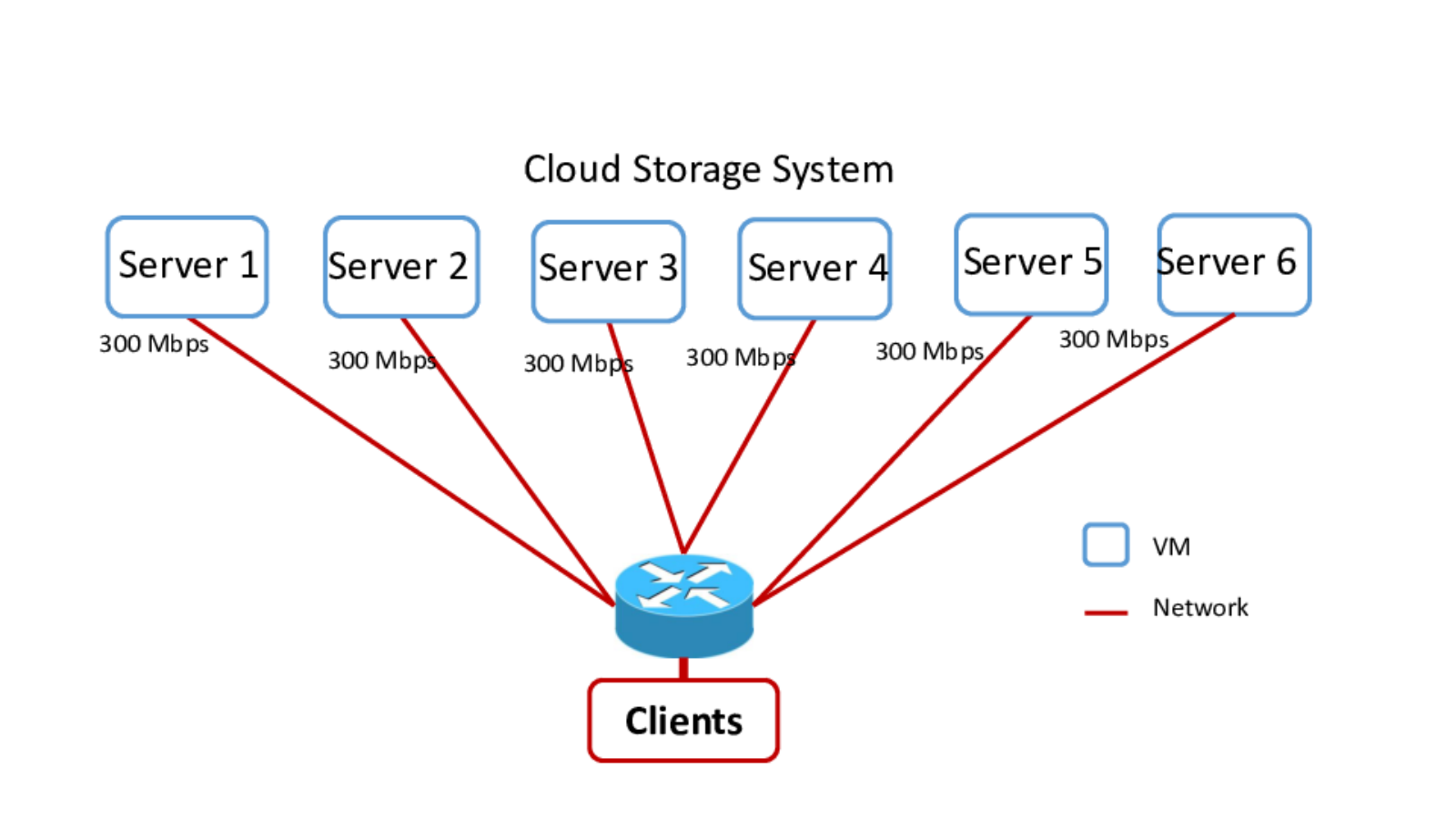
An experimental environment in a virtualized cloud environment is constructed. This virtualized cloud is managed by open source software for creating private and public cloud, Openstack. We allocated 6 virtual machines (VMs) as storage server nodes intended to store the chunks. The schematic of our testbed is illustrated in Figure 10. Table III summarizes a detailed configuration used for the experiments.
For client workload, we exploit a popular HTTP-trafic generator, Apache JMeter, with a plug-in that can generate traffic using HTTP Streaming protocol. We assume the amount of available bandwidth between origin server and each cache server is 200 Mbps, 500 Mbps between cache server 1/2 and edge router 1, and 300 Mbps between cache server 3/4/5 and edge router 2. In this experiments, to allocate bandwidth to the clients, we throttle the client (i.e., JMeter) traffic according to the plan generated by our algorithm. We consider threads (i.e., users), , and set , . We chose the code as an example for our experiment. However, any other coding setting still works given that the required resources are available. The video files are of length of seconds and the segment length is set to be s. For each segment, we used JMeter built-in reports to estimate the downloaded time of each segment and then plug these times into our model to get the needed metric.
Figure 11 shows four different policies where we compare the actual mean stall duration (MSD) for video files, analytical MSD, PSP-QTB-based MSD, PEA-QTB-based MSD and PEB-QTA-based MSD algorithms. We observe that the analytical MSD is very close to the actual measurements of the MSD obtained from our testbed, and approaches zero for reasonable large values of . Further, the proposed approach is shown to outperform the considered baselines.
VIII Conclusion
In this paper, a video streaming over cloud is considered where the content is erasure-coded on the distributed servers. We consider two quality of experience metrics to optimize: mean stall duration and average quality of the streamed video. A two-stage probabilistic scheduling is proposed for the choice of servers and the parallel streams between the server and the edge router. Using the two-stage probabilistic scheduling and probabilistic quality assignment for the videos, an upper bound on the mean stall duration is derived. An optimization problem that minimizes a convex combination of the two QoE metrics is formulated, over the choice of two-stage probabilistic scheduling, probabilistic quality assignment, bandwidth allocation, and auxiliary variables. Efficient algorithm is proposed to solve the optimization problem and the evaluation results depict the improved performance of the algorithm as compared to the considered baselines.
References
- [1] “Four reasons we choose amazon’s cloud as our computing platform,” Netflix "Tech" Blog, December, 2010.
- [2] V. Aggarwal, V. Gopalakrishnan, R. Jana, K. Ramakrishnan, and V. Vaishampayan, “Optimizing cloud resources for delivering iptv services through virtualization,” Multimedia, IEEE Transactions on, vol. 15, no. 4, pp. 789–801, June 2013.
- [3] Marketsandmarkets, “Solution, by service, by platform, by user type, by deployment type, by revenue model, by industry, and by region - global forecast to 2021,” http://www.marketsandmarkets.com/Market-Reports/video-streaming-market-181135120.html, May 2016.
- [4] D. Mowrey, “Cloud video trends to watch in 2017,” http://www.multichannel.com/blog/mcn-guest-blog/cloud-video-trends-watch-2017/409903, Jan 2017.
- [5] P. J. Denning and T. G. Lewis, “Exponential laws of computing growth,” Commun. ACM, vol. 60, no. 1, pp. 54–65, Dec. 2016. [Online]. Available: http://doi.acm.org/10.1145/2976758
- [6] H. Weatherspoon and J. Kubiatowicz, “Erasure coding vs. replication: A quantitative comparison,” in Revised Papers from the First International Workshop on Peer-to-Peer Systems, ser. IPTPS ’01. Springer-Verlag, 2002.
- [7] A. Dimakis, P. Godfrey, Y. Wu, M. Wainwright, and K. Ramchandran, “Network coding for distributed storage systems,” Information Theory, IEEE Transactions on, vol. 56, no. 9, pp. 4539–4551, Sept 2010.
- [8] M. Sathiamoorthy, M. Asteris, D. Papailiopoulos, A. G. Dimakis, R. Vadali, S. Chen, and D. Borthakur, “Xoring elephants: Novel erasure codes for big data,” in Proceedings of the 39th international conference on Very Large Data Bases., 2013.
- [9] C. Huang, H. Simitci, Y. Xu, A. Ogus, B. Calder, P. Gopalan, J. Li, and S. Yekhanin, “Erasure coding in windows azure storage,” in Proceedings of the 2012 USENIX Conference on Annual Technical Conference, ser. USENIX ATC’12. USENIX Association, 2012.
- [10] A. Fikes, “Storage architecture and challenges (talk at the google faculty summit),” http://bit.ly/nUylRW, Tech. Rep., 2010.
- [11] T.-Y. Huang, R. Johari, N. McKeown, M. Trunnell, and M. Watson, “A buffer-based approach to rate adaptation: Evidence from a large video streaming service,” ACM SIGCOMM Computer Communication Review, vol. 44, no. 4, pp. 187–198, 2015.
- [12] B. Han, F. Qian, L. Ji, and V. Gopalakrishnan, “Mp-dash: Adaptive video streaming over preference-aware multipath,” in Proceedings of the 12th International on Conference on emerging Networking EXperiments and Technologies. ACM, 2016, pp. 129–143.
- [13] N. Shah, K. Lee, and K. Ramachandran, “The mds queue: analyzing latency performance of codes and redundant requests,” arXiv:1211.5405, Nov 2012.
- [14] Y. Xiang, T. Lan, V. Aggarwal, and Y. F. R. Chen, “Joint latency and cost optimization for erasure-coded data center storage,” SIGMETRICS Perform. Eval. Rev., vol. 42, no. 2, pp. 3–14, Sep. 2014. [Online]. Available: http://doi.acm.org/10.1145/2667522.2667524
- [15] ——, “Joint latency and cost optimization for erasure-coded data center storage,” IEEE/ACM Transactions on Networking, vol. 24, no. 4, pp. 2443–2457, Aug 2016.
- [16] S. Chen, Y. Sun, U. Kozat, L. Huang, P. Sinha, G. Liang, X. Liu, and N. Shroff, “When queuing meets coding: Optimal-latency data retrieving scheme in storage clouds,” in Proceedings of IEEE Infocom, 2014.
- [17] G. Scutari, F. Facchinei, L. Lampariello, and P. Song, “Parallel and distributed methods for nonconvex optimization- part i: Theory,” IEEE Trans. Signal Process, 2014.
- [18] L. Huang, S. Pawar, H. Zhang, and K. Ramchandran, “Codes can reduce queueing delay in data centers,” in Information Theory Proceedings (ISIT), 2012 IEEE International Symposium on, July 2012, pp. 2766–2770.
- [19] G. Joshi, Y. Liu, and E. Soljanin, “On the delay-storage trade-off in content download from coded distributed storage systems,” Selected Areas in Communications, IEEE Journal on, vol. 32, no. 5, pp. 989–997, May 2014.
- [20] F. Baccelli, A. Makowski, and A. Shwartz, “The fork-join queue and related systems with synchronization constraints: stochastic ordering and computable bounds,” Advances in Applied Probability, pp. 629–660, 1989.
- [21] V. Aggarwal, J. Fan, and T. Lan, “Taming tail latency for erasure-coded, distributed storage systems,” in Proc. IEEE Infocom, Jul 2017.
- [22] V. Aggarwal, A. O. Al-Abbasi, J. Fan, and T. Lan, “Taming tail latency for erasure-coded, distributed storage systems,” CoRR, vol. abs/1703.08337, 2017. [Online]. Available: http://arxiv.org/abs/1703.08337
- [23] V. Aggarwal and T. Lan, “Tail index for a distributed storage system with pareto file size distribution,” CoRR, vol. abs/1607.06044, 2016. [Online]. Available: http://arxiv.org/abs/1607.06044
- [24] K. Lee, L. Yan, A. Parekh, and K. Ramchandran, “A vod system for massively scaled, heterogeneous environments: Design and implementation,” in 2013 IEEE 21st International Symposium on Modelling, Analysis and Simulation of Computer and Telecommunication Systems. IEEE, 2013, pp. 1–10.
- [25] Z. Huang, C. Mei, L. E. Li, and T. Woo, “Cloudstream: Delivering high-quality streaming videos through a cloud-based svc proxy,” in INFOCOM, 2011 Proceedings IEEE. IEEE, 2011, pp. 201–205.
- [26] J. He, Y. Wen, J. Huang, and D. Wu, “On the cost–qoe tradeoff for cloud-based video streaming under amazon ec2’s pricing models,” IEEE Transactions on Circuits and Systems for Video Technology, vol. 24, no. 4, pp. 669–680, 2014.
- [27] H.-Y. Chang, K.-B. Chen, and H.-C. Lu, “A novel resource allocation mechanism for live cloud-based video streaming service,” Multimedia Tools and Applications, pp. 1–18, 2016.
- [28] N. Oza and N. Gohil, “Implementation of cloud based live streaming for surveillance,” in Communication and Signal Processing (ICCSP), 2016 International Conference on. IEEE, 2016, pp. 0996–0998.
- [29] M. Chen, “Amvsc: a framework of adaptive mobile video streaming in the cloud,” in Global Communications Conference (GLOBECOM), 2012 IEEE. IEEE, 2012, pp. 2042–2047.
- [30] X. Wang, M. Chen, T. T. Kwon, L. Yang, and V. C. Leung, “Ames-cloud: a framework of adaptive mobile video streaming and efficient social video sharing in the clouds,” IEEE Transactions on Multimedia, vol. 15, no. 4, pp. 811–820, 2013.
- [31] A. O. Al-Abbasi and V. Aggarwal, “Video streaming in distributed erasure-coded storage systems: Stall duration analysis,” CoRR, vol. abs/1703.08348, 2017. [Online]. Available: http://arxiv.org/abs/1703.08348
- [32] A. Zwart and O. J. Boxma, “Sojourn time asymptotics in the m/g/1 processor sharing queue,” Queueing systems, vol. 35, no. 1-4, pp. 141–166, 2000.
- [33] M. Kuczma, An introduction to the theory of functional equations and inequalities: Cauchy’s equation and Jensen’s inequality. Springer Science & Business Media, 2009.
- [34] B. C. Arnold, Pareto distribution. Wiley Online Library, 2015.
- [35] V. Ramaswami, K. Jain, R. Jana, and V. Aggarwal, “Modeling heavy tails in traffic sources for network performance evaluation,” in Computational Intelligence, Cyber Security and Computational Models, ser. Advances in Intelligent Systems and Computing. Springer India, 2014, vol. 246, pp. 23–44.
- [36] C. Kreuzberger, D. Posch, and H. Hellwagner, “A scalable video coding dataset and toolchain for dynamic adaptive streaming over http,” in Proceedings of the 6th ACM Multimedia Systems Conference. ACM, 2015, pp. 213–218.
Appendix A Algorithm Pseudo-codes for the Sub-problems
- 1.
Initialize , ,, , such that is feasible ,
- 2.
while
- 3.
//Solve for with given
- 4.
Step 1: Compute the solution of s.t. , , , , , solved using projected gradient descent
- 5.
Step 2: .
- 6.
//update index
- 7.
Set
- 8.
end while
- 9.
output:
- 1.
Initialize , , , such that is feasible,
- 2.
while
- 3.
//Solve for with given
- 4.
- 5.
Step 2: .
- 6.
//update index
- 7.
Set
- 8.
end while
- 9.
output:
- 1.
Initialize , , , such that is feasible,
- 2.
while
- 3.
//Solve for with given
- 4.
- 5.
Step 2: .
- 6.
//update index
- 7.
Set
- 8.
end while
- 9.
output:
- 1.
Initialize , , , such that is feasible,
- 2.
while
- 3.
//Solve for with given
- 4.
- 5.
Step 2: .
- 6.
//update index
- 7.
Set
- 8.
end while
- 9.
output:
- 1.
Initialize , , , such that is feasible,
- 2.
while
- 3.
//Solve for with given
- 4.
- 5.
Step 2: .
- 6.
//update index
- 7.
Set
- 8.
end while
- 9.
output: