Stability and Error Estimates of BV Solutions
to the Abel Inverse Problem

Linan Zhang Affiliation: Department of Mathematical Sciences, Carnegie Mellon University, Pittsburgh, PA 15213. (linanz@andrew.cmu.edu, schaeffer@cmu.edu) Hayden Schaeffer Affiliation: Department of Mathematical Sciences, Carnegie Mellon University, Pittsburgh, PA 15213. (linanz@andrew.cmu.edu, schaeffer@cmu.edu)

June, 2018

Abstract

Reconstructing images from ill-posed inverse problems often utilizes total variation regularization in order to recover discontinuities in the data while also removing noise and other artifacts. Total variation regularization has been successful in recovering images for (noisy) Abel transformed data, where object boundaries and data support will lead to sharp edges in the reconstructed image. In this work, we analyze the behavior of $BV$ solutions to the Abel inverse problem, deriving a priori estimates on the recovery. In particular, we provide $L^{2}$ -stability bounds on $BV$ solutions to the Abel inverse problem. These bounds yield error estimates on images reconstructed from a proposed total variation regularized minimization problem.

1 Introduction

The Abel integral equation arises in a variety of fields, including medical imaging, astronomy, geophysics, and electron microscopy [22, 31, 8, 19]. The Abel equation is an essential tool in many aspects of science, since internal structures (such as density, composition, velocity profiles, etc.) of an object can be reconstructed from just their line-of-sight projections, with the assumption that the structures are axisymmetric or nearly-axisymmetric. The reconstruction, i.e. the inversion of the Abel integral equation, is an ill-posed problem due to a lack of smoothness in the data and solution (typically in the form of discontinuities along object or material boundaries) and the presence of random additive noise.

In practice, several analytical and numerical approaches were proposed to (essentially) deconvolve the integral equation. In [23, 38], the authors used the Abel-Fourier-Hankel cycle [8] to solve the inverse problem. This is based on the projection-slice theorem and uses a special relationship between the Abel and Fourier transforms. In [18, 28], the authors used a basis-set expansion (either on the solution or the projection) to solve the inverse problem, where the action of the Abel transform is analytically calculated on each basis functions and the coefficients are solved computationally. It is noted that the linear system for the coefficients required Tikhonov regularization to avoid ill-conditioning. Other approaches include the Cormack inversion [15, 16, 39] and the onion-peeling method [17, 32]. Without additional regularization, these methods tend to amplify noise due to the ill-conditioning of the discrete inverse problem. This is a result of the ill-posedness of the continuous problem [22, 31]. In addition, these methods are often not suitable for discontinuous data.

To handle discontinuities and noise, it is natural to consider restricting solutions to functions of bounded variation. This is done by adding a total variation penalty on the inverse problem. Total variation (TV) regularization is an essential part of many inversion methods in image processing, originating from the ROF model [33] for denoising, and now popular in many models, including, for example: compressive sensing and medical imaging [10, 9, 27], video processing [26, 25, 41, 36, 37], and cartoon-texture decomposition [29, 30, 35]. Let $\mathcal{A}$ be the Abel transform, $f$ be the line-of-sight projection of some unknown non-negative axisymmetric function $u$ , and $\Omega\subset\mathbb{R}^{2}$ be the compact support of $f$ . In [4, 5], the authors presented the following TV regularized minimization problem:

\displaystyle\min_{u\in BV(U)}\quad

\displaystyle\|u\|_{TV(U)}+\dfrac{\lambda}{2}\|\mathcal{A}u-f\|_{L^{2}(\Omega)}^{2},

(1.1)

where $U$ is the rotation of $\Omega$ about the $z$ -axis, and thus the TV semi-norm (for axisymmetric functions) is defined as follows:

\displaystyle\|u\|_{TV(U)}:=\sup\left\{\iint_{\Omega}u(r,z)\dir(r\phi(r,z))\differential{r}\differential{z}:\phi\in C_{c}^{1}(\Omega;\mathbb{R}^{2}),\,\|\phi\|_{L^{\infty}(\Omega)}\leq 1\right\},

where the divergence is calculated with respect to the variables $(r,z)$ . In [4], it was shown that if $f\in L^{2}(\Omega)$ , then Problem (1.1) has a unique global minimizer in $BV(U)$ . In addition, numerical results on discontinuous functions showed that solving Equation (1.1) yields better results versus unregularized inversion or $H^{1}$ regularized inversion. In [14], the variational model in Equation (1.1) was modified by adding the box constraint:

\begin{split}\min_{u\in BV(U)}\quad&\|u\|_{TV(U)}+\dfrac{\lambda}{2}\|\mathcal{A}u-f\|_{L^{2}(\Omega)}^{2}\\ \text{subject to}\quad&u\in[a,b]\text{ on }U,\end{split}

which was noted to have better denoising results than the model without the constraint. In [1], the authors proved existence and/or uniqueness results for various models, including the binary minimization problem:

\begin{split}\min_{u\in BV(\Omega)}\quad&\|u\|_{TV(\Omega)}+\dfrac{\lambda}{2}\|\mathcal{A}u-f\|_{L^{2}(\Omega)}^{2}\\ \text{subject to}\quad&u\in\{0,1\}\text{ a.e. on }\Omega,\end{split}

where the TV semi-norm over $\Omega$ is defined as follows:

\displaystyle\|u\|_{TV(\Omega)}:=\sup\left\{\iint_{\Omega}u(r,z)\dir\phi(r,z)\differential{r}\differential{z}:\phi\in C_{c}^{1}(\Omega;\mathbb{R}^{2}),\,\|\phi\|_{L^{\infty}(\Omega)}\leq 1\right\}.

Additionally, a higher-order TV regularization for the Abel inverse problem was proposed in [13], where the regularization term is the sum of the TV semi-norm and the $L^{1}$ norm of the Laplacian. Numerical experiments showed that the addition of the $L^{1}$ norm of the Laplacian helps to recover piecewise smooth data as opposed to piecewise constant data typically recovered by TV regularized inversion. In each of these variational models, the main regularization involves the TV semi-norm, thus resulting in $BV$ solutions. In addition, the data is fit with respect to the $L^{2}$ norm. Therefore, one would expect to control the $L^{2}$ -error between an approximation and the true image by the TV semi-norm of the solution and the $L^{2}$ norm of the given data.

1.1 Contributions of this work

Motivated by the various total variation regularized Abel inversion models, we provide analytic and numerical results on the behavior of $BV$ solutions of the Abel inverse problem. Since many of the related variational models involve the TV semi-norm and an $L^{2}$ data-fit, we derive error bounds using these terms.

In particular, we provide a priori $L^{2}(U)$ -stability bounds of $BV$ solutions, and from these estimates, we derive an $L^{2}(U)$ -error estimate when regularizing the inverse problem by $\|u\|_{TV(\Omega)}$ (the total variation of the solution in cylindrical coordinates). Amongst the choices of TV-regularizers for the Abel inverse problem, our analysis shows that $\|u\|_{TV(\Omega)}$ naturally arises as an error control term. The motivation for $L^{2}$ -error bounds comes from the fact that many recovery results are measured by the root-mean squared error. Several numerical examples verify that our variational model and error bound yields satisfactory results.

Our derivation also yields an $L^{1}(U)$ -stability bound of $BV$ solutions, which agrees (and simplifies) the $L^{1}$ -bound for 1D problems found in [22]. Note that the $L^{2}$ -bounds in [22] do not apply to $BV$ solutions, and extensions of the results in [22] can be shown to be suboptimal for the problem considered in this work. Therefore, we have derived different and new bounds which are applicable to the problem considered here. In addition, we present the first error results for $BV$ solutions that hold for 1D and 2D data (with 2D and 3D solutions respectively).

1.2 Overview

This paper is organized as follows. In Section 2, we discuss the Abel inverse problem and a TV regularized model. In Section 3, we derive stability and error bounds for $BV$ solutions in both two and three dimensions. In Section 4, some examples are shown, which verify the theoretical estimates.

2 Inverse Problem and Variational Method

In this section, we define the Abel integral operator as well as a variational model used for the inversion. Although there are several choices for the variational model, the particular one used here naturally occurs within our analysis.

Definition 2.1.

Let $u:\mathbb{R}^{2}\to\mathbb{R}$ be an axisymmetric function. The Abel transform of $u$ is defined as:

\displaystyle\mathcal{A}u(x):=2\int_{x}^{\infty}\dfrac{u(r)r}{\sqrt{r^{2}-x^{2}}}\differential{r},\quad x\in\mathbb{R}^{+}.

(2.1)

If $u:\mathbb{R}^{3}\to\mathbb{R}$ is an axisymmetric function, then the Abel transform of $u$ is defined as:

\displaystyle\mathcal{A}u(x,z):=2\int_{x}^{\infty}\dfrac{u(r,z)r}{\sqrt{r^{2}-x^{2}}}\differential{r},\quad(x,z)\in\mathbb{R}^{+}\times\mathbb{R}.

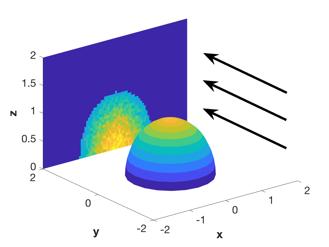
Refer to caption — Figure 2.1: Graphical description of the Abel transform. The axisymmetric object (with compact support) is integrated along lines parallel to the $y$ -axis, and a line-of-sight projection is obtained. The line of sight is illustrated by the arrows. The projection on the $(x,z)$ -plane contains noise due to measurement error. The inverse problem is to reconstruct the 3D object from the 2D projection.

Let $u$ be the unknown density of an axisymmetric object and suppose that we are given data $f$ , which is the line-of-sight projection of $u$ onto a co-dimension one domain (see Figure 2.1). In this work, we always assume that $u$ is non-negative. To reconstruct $u$ from $f$ , one can solve the following linear system:

\displaystyle f=\mathcal{A}u.

(P_A)

This is known as the Abel integral equation. We also assume that the data and solution are compactly supported within the domain of interest. The solution may have discontinuities along object boundaries or may have jumps at the support boundary, thus $BV$ solutions should be expected.

In Theorems 3.3 and 3.12, it is shown that if the function $f$ is of bounded variation, then Problem (PA) has a unique solution in $L^{1}$ . However, to ensure the solutions are in $BV$ , we consider the TV regularized problem:

\displaystyle\min_{u\in BV(\Omega)}\quad

\displaystyle\|u\|_{TV(\Omega)}+\dfrac{\lambda}{2}\|\mathcal{A}u-f\|_{L^{2}(\Omega)}^{2},

(P_TV)

where $f$ is the given data with compact support $\Omega\subset\mathbb{R}^{d}$ , $d\in\{1,2\}$ , and $\|u\|_{TV(\Omega)}$ is the total variation of $u$ in $\Omega$ and is defined by:

\displaystyle\|u\|_{TV(\Omega)}:=\sup\left\{\int_{\Omega}u(r)\dir\phi(r)\differential{r}:\phi\in C_{c}^{1}(\Omega;\mathbb{R}^{2}),\,\|\phi\|_{L^{\infty}(\Omega)}\leq 1\right\}

(2.2)

if $d=1$ , or

\displaystyle\|u\|_{TV(\Omega)}:=\sup\left\{\iint_{\Omega}u(r,z)\dir\phi(r,z)\differential{r}\differential{z}:\phi\in C_{c}^{1}(\Omega;\mathbb{R}^{2}),\,\|\phi\|_{L^{\infty}(\Omega)}\leq 1\right\}

(2.3)

if $d=2$ . Let $u^{*}$ be the minimizer to Problem (PTV). Informally, the regularization term $\|u\|_{TV(\Omega)}$ ensures that $u^{*}\in BV(\Omega)$ and allows for discontinuities in the radial profile, and the loss term $\|\mathcal{A}u-f\|_{L^{2}(\Omega)}^{2}$ enforces that $\mathcal{A}u^{*}\approx f$ in the presence of Gaussian noise.

Remark 2.2.

Problem (PTV) differs from Problem (1.1) in that the regularization term in Problem (PTV) is the total variation of $u$ with respect to the cylindrical coordinates, while the regularization term in Problem (1.1) is the total variation of $u$ with respect to the Cartesian coordinates. See Proposition C.1.

Without loss of generality, assume that the support of the data is contained in $[0,1)\subset\mathbb{R}$ , if the data is 1D, or $[0,1)\times[-1,1]\subset\mathbb{R}^{2}$ , if the data is 2D. The results developed in the subsequent sections can be generalized to any bounded domain in the same form by introducing an additional constant depending only on the size of the domain. We denote $\Omega=[0,1]\times[-1,1]\subset\mathbb{R}^{2}$ , $\Omega_{h}=[h,1]\times[-1,1]\subset\mathbb{R}^{2}$ where $h\in(0,1/2]$ , and $U=\{(x,y)\in\mathbb{R}^{2}:x^{2}+y^{2}\leq 1\}\times[-1,1]\subset\mathbb{R}^{3}$ in order to simplify the notations.

3 Stability and Error Estimates

In this section, we analyze the stability of $BV$ solutions to Problem (PA) and estimate the error of $BV$ solutions to Problem (PTV). In particular, we show that given a minimizer of Problem (PTV), we can control the $L^{2}$ norm of the solution in terms of a fixed multiple of the $L^{2}$ norm of the data. This provides a quantitative error bound that is not common for this type of model. The stability estimates derived in this work are:

\displaystyle\|u\|_{L^{2}(B(0,1))}

\displaystyle\leq C\|u\|_{TV(0,1)}^{1/2}\|f\|_{L^{2}(0,1)}^{1/2}

if the data is 1D (solutions are 2D), and

\displaystyle\|u\|_{L^{2}(U)}

\displaystyle\leq C\|u\|_{L^{\infty}(\Omega)}^{1/3}\|u\|_{TV(\Omega)}^{1/3}\|f\|_{L^{2}(\Omega)}^{1/3}

if the data is 2D (solutions are 3D). Note that the right-hand side of the inequalities are expressed in terms of norms and semi-norms over co-dimension one regions. These bounds yield an error estimate for Problem (PTV).

The motivation for deriving $L^{2}$ -bounds is to provide variance control over the $BV$ regularized least-squares solution. In practical applications, the fit of the recovered solution is measured by the root-mean squared error. Therefore, it is natural to look for a theoretical bound on the $L^{2}$ -error. In related variational models, the recovered images are assumed to be in $BV$ , and the data-fit is measured by the $L^{2}$ norm. Thus, our error bounds can be controlled by the (easily available) TV semi-norm of the solution and the $L^{2}$ norm of the given data.

We first introduce the following integral transform for functions, which is known as the Weyl fractional integral of order $1/2$ and is closely related to the Abel transform [31].

Definition 3.1.

Let $v$ be a scalar-valued function defined on $\mathbb{R}^{+}$ . The $\mathcal{J}$ -transform of $v$ is defined as:

\displaystyle\mathcal{J}v(x):=\dfrac{1}{\sqrt{\pi}}\int_{x}^{\infty}\dfrac{v(r)}{\sqrt{r-x}}\differential{r},\quad x\in\mathbb{R}^{+}.

(3.1)

If $v$ is a scalar-valued function defined on $\mathbb{R}^{+}\times\mathbb{R}$ , the $\mathcal{J}$ -transform of $v$ is defined as:

\displaystyle\mathcal{J}v(x,z):=\dfrac{1}{\sqrt{\pi}}\int_{x}^{\infty}\dfrac{v(r,z)}{\sqrt{r-x}}\differential{r},\quad(x,z)\in\mathbb{R}^{+}\times\mathbb{R}.

(3.2)

Let $v$ be an unknown function defined on $\mathbb{R}^{+}$ or $\mathbb{R}^{+}\times\mathbb{R}$ , and suppose that we are given the $\mathcal{J}$ -transform of $v$ , denoted by $g$ . An analogy to the Abel integral equation (PA) is the following:

\displaystyle g=\mathcal{J}v.

(P_J)

The connection between Problems (PA) and (PJ) is shown in Sections 3.1 and 3.2. In this work, we assume that $v$ is also non-negative.

In the following subsections, we will focus on $L^{2}$ -stability estimates of $BV$ solutions to Problems (PA) and (PJ), and for the sake of completeness, we will provide the corresponding $L^{1}$ -stability estimates in Appendix A.

3.1 $L^{2}$ -Stability Estimates for $BV$ Solutions in 2D

Before analyzing the stability of $BV$ solutions to Problem (PA), we discuss the existence and uniqueness of solutions to the inverse problem over different spaces of functions as well as the relationship between the Abel transform and the $\mathcal{J}$ -transform.

Assume that $u:\mathbb{R}^{2}\to\mathbb{R}$ is an axisymmetric function which is compactly supported within the ball $B(0,1)\subset\mathbb{R}^{2}$ , and that $v:\mathbb{R}^{+}\to\mathbb{R}$ is defined as $v(r^{2})=u(r)$ . Changing variables shows that:

\displaystyle\mathcal{A}u(x)

\displaystyle=2\int_{x}^{1}\dfrac{u(r)r}{\sqrt{r^{2}-x^{2}}}\differential{r}=\int_{x^{2}}^{1}\dfrac{u(\sqrt{r})}{\sqrt{r-x^{2}}}\differential{r}=\sqrt{\pi}\mathcal{J}v(x^{2}),\quad x\in[0,1].

(3.3)

The analysis of Problem (PJ) can thus be related back to the Abel inverse problem through a simple change of variables. The following theorem states the existence and uniqueness of solutions to Problem (PJ).

Theorem 3.2.

(restated from [22]) Problem (PJ) has a unique solution in $L^{1}(0,1)$ , which is given by:

\displaystyle v(r)=-\dfrac{1}{\sqrt{\pi}}\int_{r}^{1}\dfrac{\differential{g(x)}}{\sqrt{x-r}},

(3.4)

provided that the function $g$ is of bounded variation, $0\leq g(0)<\infty$ , and ${\rm supp}(g)\subset[0,1)$ . Here the integral is in the Lebesgue-Stieltjes sense.

The proof of Theorem 3.2 appears in Appendix C. An analogy of Theorem 3.2 for Problem (PA) can be derived immediately from Equations (3.3) and (3.4).

Theorem 3.3.

Problem (PA) has a unique solution in $L^{1}(0,1)$ , which is given by:

\displaystyle u(r)=-\dfrac{1}{\pi}\int_{r}^{1}\dfrac{\differential{f(x)}}{\sqrt{x^{2}-r^{2}}},

provided that the function $f$ is of bounded variation, $0\leq f(0)<\infty$ , and ${\rm supp}(f)\subset[0,1)$ .

Theorems 3.2 and 3.3 guarantee only that the solution exists in $L^{1}$ . If it is known a priori that the solution is in $BV$ , then it can be shown that the data is Hölder continuous.

Theorem 3.4.

(restated from [6]) The operator $\mathcal{J}$ defined by Equation (3.1) is a continuous operator from $BV(0,1)$ into $C^{0,1/2}(0,1)$ .

Here $C^{0,1/2}$ denotes the space of all functions on $[0,1]$ which satisfy the Hölder condition of order $1/2$ . This result is a direct consequence of Proposition C.5 and Poincaré’s inequality in 1D. An analogy of Theorem 3.4 can be derived immediately from Equation (3.3).

Corollary 3.5.

The operator $\mathcal{A}$ defined by Equation (2.1) is a continuous operator from $BV(0,1)$ into $C^{0,1/2}(0,1)$ .

The statement above shows that, in practice, one may need to regularize the Abel inverse problem in order to ensure that the solutions are in $BV$ .

We now focus on the stability of $BV$ solutions to Problems (PA) and (PJ). The following lemma provides two basic estimates for the “running average,” $v_{h}$ , of a function $v$ defined on the interval $[0,1]\subset\mathbb{R}$ , where $h\in(0,1/2]$ . The introduction of the auxiliary function $v_{h}$ helps us to bound $v$ in $L^{2}(h,1)$ , with a bound that is a function of $h$ . Then one can minimize the bound in $h$ over $(0,1/2]$ to obtain a bound of $v$ in $L^{2}(0,1)$ .

Lemma 3.6.

Let $v\in W^{1,1}(0,1)$ . Let $h\in(0,1/2]$ and define $v_{h}:[h,1]\to\mathbb{R}$ by:

\displaystyle v_{h}(x):=\dfrac{1}{h}\int_{x-h}^{x}v(y)\differential{y}.

(3.5)

Then the following two estimates hold:

	$\displaystyle\\|v-v_{h}\\|_{L^{2}(h,1)}$	$\displaystyle\leq 3^{-1/2}h^{1/2}\\|v^{\prime}\\|_{L^{1}(0,1)},$		(3.6)
	$\displaystyle\\|v_{h}\\|_{L^{\infty}(h,1)}$	$\displaystyle\leq\\|v\\|_{L^{\infty}(0,1)}.$		(3.7)

Proof.

We first verify that $v_{h}-v$ can be written as a convolution for $x\in[h,1]$ :

\displaystyle v_{h}(x)-v(x)

\displaystyle=\int_{0}^{1}v^{\prime}(y)\left(\dfrac{x-y}{h}-1\right)\mathds{1}_{[0,h]}(x-y)\differential{y}.

(3.8)

Since $v\in W^{1,1}(0,1)$ , it is absolutely continuous, and by the fundamental theorem of calculus, we have:

	$\displaystyle\int_{0}^{1}v^{\prime}(y)\left(\dfrac{x-y}{h}-1\right)\mathds{1}_{[0,h]}(x-y)\differential{y}$	$\displaystyle=\int_{x-h}^{x}v^{\prime}(y)\left(\dfrac{x-y}{h}\right)\differential{y}-\int_{x-h}^{x}v^{\prime}(y)\differential{y}$
		$\displaystyle=-v(x-h)+\dfrac{1}{h}\int_{x-h}^{x}v(y)\differential{y}-\left(v(x)-v(x-h)\right)$
		$\displaystyle=v_{h}(x)-v(x).$

It can be seen from Equation (3.8) that $v_{h}-v=K*g$ on $[h,1]$ , where

\displaystyle K(x):=\left(\dfrac{x}{h}-1\right)\mathds{1}_{[0,h]}(x),\quad g(x):=v^{\prime}(x)\mathds{1}_{[0,1]}(x),

and we have extended the functions to $\mathbb{R}$ . Applying Young’s inequality for convolutions, we obtain:

\displaystyle\|v-v_{h}\|_{L^{2}(h,1)}=\|K*g\|_{L^{2}(h,1)}\leq\|K*g\|_{L^{2}(\mathbb{R})}\leq\|K\|_{L^{2}(\mathbb{R})}\|g\|_{L^{1}(\mathbb{R})}=3^{-1/2}h^{1/2}\|v^{\prime}\|_{L^{1}(0,1)},

where the last equality can be calculated directly. This shows Equation (3.6).

By Equation (3.5), for $x\in[h,1]$ ,

\displaystyle|v_{h}(x)|\leq\dfrac{1}{h}\int_{x-h}^{x}|v(y)|\differential{y}\leq\|v\|_{L^{\infty}(0,1)},

which shows Equation (3.7). ∎

Remark 3.7.

One could obtain an alternative bound for $\|v-v_{h}\|_{L^{2}(h,1)}$ by using the $L^{p}$ embedding theorem and Poincaré’s inequality in 1D:

	$\displaystyle\\|v-v_{h}\\|_{L^{2}(h,1)}$	$\displaystyle\leq\\|v\\|_{L^{2}(h,1)}+\\|v_{h}\\|_{L^{2}(h,1)}\leq(1-h)^{1/2}\left(\\|v\\|_{L^{\infty}(h,1)}+\\|v_{h}\\|_{L^{\infty}(h,1)}\right)$
		$\displaystyle\leq 2(1-h)^{1/2}\\|v\\|_{L^{\infty}(0,1)}\leq 2(1-h)^{1/2}\\|v^{\prime}\\|_{L^{1}(0,1)}.$		(3.9)

Note that $3^{-1/2}h^{1/2}<2(1-h)^{1/2}$ for $h\in(0,1/2]$ , so that the estimate in Equation (3.9) is not as tight as the estimate in Equation (3.6). In addition, Equation (3.9) could lead to complications in later arguments.

The following theorem shows a stability estimate for $W^{1,1}$ solutions to Problem (PJ) in terms of the data itself.

Theorem 3.8.

If $v\in W^{1,1}(0,1)$ with ${\rm supp}(v)\subset[0,1)$ and $\mathcal{J}v=g$ , we have:

\displaystyle\|v\|_{L^{2}(0,1)}\leq C\|v^{\prime}\|_{L^{1}(0,1)}^{1/2}\|g\|_{L^{2}(0,1)}^{1/2},

(3.10)

where $C$ is a constant independent of $v$ .

Proof.

We first note that for each $x\in[0,1]$ , Fubini’s theorem implies that

	$\displaystyle\mathcal{J}^{2}v(x)$	$\displaystyle=\dfrac{1}{\sqrt{\pi}}\int_{x}^{1}\dfrac{\mathcal{J}v(s)}{\sqrt{s-x}}\differential{s}=\dfrac{1}{\pi}\int_{x}^{1}\dfrac{1}{\sqrt{s-x}}\int_{s}^{1}\dfrac{v(y)}{\sqrt{y-s}}\differential{y}\differential{s}$
		$\displaystyle=\dfrac{1}{\pi}\int_{x}^{1}v(y)\int_{x}^{y}\dfrac{1}{\sqrt{s-x}\sqrt{y-s}}\differential{s}\differential{y}=\int_{x}^{1}v(y)\differential{y},$		(3.11)

where the last step follows from Equation (C.1). This is the key to the argument, specifically, that two applications of $\mathcal{J}$ is the same as integration. Then from Equations (3.5) and (3.11), we have, for $x\in[h,1]$ ,

$\displaystyle\sqrt{\pi}hv_{h}(x)$	$\displaystyle=\sqrt{\pi}\left(\int_{x-h}^{1}v(y)\differential{y}-\int_{x}^{1}v(y)\differential{y}\right)=\sqrt{\pi}\left(\mathcal{J}g(x-h)-\mathcal{J}g(x)\right)$
	$\displaystyle=\int_{x-h}^{1}\dfrac{g(y)}{\sqrt{y-(x-h)}}\differential{y}-\int_{x}^{1}\dfrac{g(y)}{\sqrt{y-x}}\differential{y}$
	$\displaystyle=\int_{x-h}^{x}\dfrac{g(y)}{\sqrt{y-(x-h)}}\differential{y}+\int_{x}^{1}g(y)\left[\dfrac{1}{\sqrt{y-(x-h)}}-\dfrac{1}{\sqrt{y-x}}\right]\differential{y}$
	$\displaystyle=\int_{0}^{1}g(y)K_{1}(x,y)\differential{y}+\int_{0}^{1}g(y)K_{2}(x,y)\differential{y}$
	$\displaystyle=:F_{1}(x)+F_{2}(x),$	(3.12)

where we extend the kernels to the entire domain and define them by:

\displaystyle K_{1}(x,y):=\dfrac{\mathds{1}_{[0,h]}(x-y)}{\sqrt{h-(x-y)}},\quad K_{2}(x,y):=\dfrac{\mathds{1}_{[0,h]}(y-x)}{\sqrt{y-(x-h)}}-\dfrac{\mathds{1}_{[0,h]}(y-x)}{\sqrt{y-x}}.

Note that the support set $[0,h]$ in $K_{2}$ is a by-product of the assumption $x\in[h,1]$ . Since the kernels are in $L^{1}$ :

	$\displaystyle\int_{0}^{1}\|K_{1}(x,y)\|\differential{y}$	$\displaystyle=\int_{0}^{1}\|K_{1}(x,y)\|\differential{x}=2h^{1/2},$
	$\displaystyle\&\quad\int_{0}^{1}\|K_{2}(x,y)\|\differential{y}$	$\displaystyle=\int_{0}^{1}\|K_{2}(x,y)\|\differential{x}=2\left(2-\sqrt{2}\right)h^{1/2},$

and by, for example, Theorem 6.18 in [21], we have $L^{2}$ control over each term in Equation (3.12):

\displaystyle\|F_{1}\|_{L^{2}(h,1)}\leq 2h^{1/2}\|g\|_{L^{2}(0,1)},\quad\|F_{2}\|_{L^{2}(h,1)}\leq 2\left(2-\sqrt{2}\right)h^{1/2}\|g\|_{L^{2}(0,1)}.

(3.13)

Combining Equations (3.12)-(3.13), we obtain:

\displaystyle\|v_{h}\|_{L^{2}(h,1)}\leq 2\left(3-\sqrt{2}\right)\pi^{-1/2}h^{-1/2}\|g\|_{L^{2}(0,1)}.

(3.14)

On the other hand, using the $L^{p}$ interpolation theorem and Poincaré’s inequality in 1D, we obtain:

\displaystyle\|v\|_{L^{2}(0,h)}

\displaystyle\leq h^{1/2}\|v\|_{L^{\infty}(0,h)}\leq h^{1/2}\|v\|_{L^{\infty}(0,1)}\leq h^{1/2}\|v^{\prime}\|_{L^{1}(0,1)}.

(3.15)

Thus, by the triangle inequality and Equations (3.6) and (3.14)-(3.15), we have:

$\displaystyle\\|v\\|_{L^{2}(0,1)}$	$\displaystyle\leq\\|v\\|_{L^{2}(0,h)}+\\|v-v_{h}\\|_{L^{2}(h,1)}+\\|v_{h}\\|_{L^{2}(h,1)}$
	$\displaystyle\leq\left(1+1/\sqrt{3}\right)h^{1/2}\\|v^{\prime}\\|_{L^{1}(0,1)}+2\left(3-\sqrt{2}\right)\pi^{-1/2}h^{-1/2}\\|g\\|_{L^{2}(0,1)}$
	$\displaystyle\leq 2\left(1+1/\sqrt{3}\right)h^{1/2}\\|v^{\prime}\\|_{L^{1}(0,1)}+2\left(3-\sqrt{2}\right)\pi^{-1/2}h^{-1/2}\\|g\\|_{L^{2}(0,1)},$	(3.16)

where the last step follows from slightly extending the upper bound, since we will optimize Equation (3.16) with the constraint $h\in(0,1/2]$ . By direct calculation, the value $h^{*}$ that minimizes the right-hand side of Equation (3.16) is given by:

\displaystyle h^{*}=\dfrac{\left(3-\sqrt{2}\right)\|g\|_{L^{2}(0,1)}}{\sqrt{\pi}\left(1+1/\sqrt{3}\right)\|v^{\prime}\|_{L^{1}(0,1)}}.

(3.17)

We can verify that the minimizer, which depends on the factor $\|g\|_{L^{2}(0,1)}\|v^{\prime}\|_{L^{1}(0,1)}^{-1}$ , satisfies the constraint $h^{*}\in(0,1/2]$ as follows. By Equation (3.1) and integrating by parts, we have, for $x\in[0,1]$ ,

\displaystyle g(x)=\dfrac{1}{\sqrt{\pi}}\int_{x}^{1}\dfrac{v(y)}{\sqrt{y-x}}\differential{y}

\displaystyle=-\dfrac{2}{\sqrt{\pi}}\int_{x}^{1}v^{\prime}(y)\sqrt{|x-y|}\differential{y},

(3.18)

since the assumption is that ${\rm supp}(v)\subset[0,1)$ . To bound $g$ in $L^{2}(0,1)$ by $\|v^{\prime}\|_{L^{1}(0,1)}$ , we apply Young’s inequality for convolutions with

\displaystyle K(x):=-\dfrac{2}{\sqrt{\pi}}\sqrt{|x|}\mathds{1}_{[0,1]}(-x),\quad f(x):=v^{\prime}(x)\mathds{1}_{[0,1]}(x).

(3.19)

Thus $g=K*f$ on $[0,1]$ and, with $K$ and $f$ extended to $\mathbb{R}$ ,

\displaystyle\|g\|_{L^{2}(0,1)}=\|K*f\|_{L^{2}(0,1)}\leq\|K*f\|_{L^{2}(\mathbb{R})}\leq\|K\|_{L^{2}(\mathbb{R})}\|f\|_{L^{1}(\mathbb{R})}=\sqrt{2/\pi}\|v^{\prime}\|_{L^{1}(0,1)},

(3.20)

where the last step can be calculated directly. Therefore, combining Equations (3.17) and (3.20) yields:

\displaystyle h^{*}=\dfrac{\left(3-\sqrt{2}\right)\|g\|_{L^{2}(0,1)}}{\sqrt{\pi}\left(1+1/\sqrt{3}\right)\|v^{\prime}\|_{L^{1}(0,1)}}\leq\dfrac{3\sqrt{2}-2}{\pi\left(1+1/\sqrt{3}\right)}\leq\dfrac{1}{2}.

Therefore, by optimizing Equation (3.16) over $h$ , we obtain:

\displaystyle\|v\|_{L^{2}(0,1)}\leq 2\pi^{-1/4}\left(1+1/\sqrt{3}\right)^{1/2}\left(3-\sqrt{2}\right)^{1/2}\|v^{\prime}\|_{L^{1}(0,1)}^{1/2}\|g\|_{L^{2}(0,1)}^{1/2},

which gives Equation (3.10). ∎

The utility of the stability bound in Equation (3.10) is that the right-hand side of the inequality is of the form of a product-bound depending on the data, which can be calculated in practice. As an example, consider the function $v_{k}(r)=\chi(kr)$ , $k\geq 1$ , where $\chi$ is the indicator function of the interval $[0,1]$ :

\displaystyle\chi(x)=\begin{cases}1,\quad\text{if }x\in[0,1],\\ 0,\quad\text{otherwise}.\end{cases}

This is a prototypical example related to image recovery. Define $g_{k}:=\mathcal{J}v_{k}$ . It can be shown, by Equation (3.1), that:

\displaystyle g_{k}(x)=2\pi^{-1/2}(1/k-x)^{1/2}\chi(kx).

For $k\geq 1$ , it is easy to show that $\|v^{\prime}_{k}\|_{L^{1}(0,1)}=1$ , and

	$\displaystyle\\|v_{k}\\|_{L^{1}(0,1)}$	$\displaystyle=k^{-1},\quad\\|g_{k}\\|_{L^{1}(0,1)}=\dfrac{4}{3\sqrt{\pi}}k^{-3/2},$
	$\displaystyle\\|v_{k}\\|_{L^{2}(0,1)}$	$\displaystyle=k^{-1/2},\quad\\|g_{k}\\|_{L^{2}(0,1)}=\dfrac{\sqrt{2}}{\sqrt{\pi}}k^{-1}.$

If the bound on $\|v\|_{L^{2}(0,1)}$ is in the sum-form:

\displaystyle\|v\|_{L^{2}(0,1)}

\displaystyle\leq C_{1}\|v^{\prime}\|_{L^{1}(0,1)}+C_{2}\|g\|_{L^{2}(0,1)}

(3.21)

with constants $C_{1}$ and $C_{2}$ , then:

\displaystyle\lim_{k\to\infty}\|v_{k}\|_{L^{2}(0,1)}\leq C_{1}\lim_{k\to\infty}\|v^{\prime}_{k}\|_{L^{1}(0,1)}+C_{2}\lim_{k\to\infty}\|g_{k}\|_{L^{2}(0,1)}=C_{1},

which is suboptimal since $\lim_{k\to\infty}\|v_{k}\|_{L^{2}(0,1)}=0$ . On the other hand, Equation (3.10) yields $\|v_{k}\|_{L^{2}(0,1)}\leq Ck^{-1/2}$ , which obtains the correct decay rate for this example. Therefore, in terms of applicability, a sum-bound in the form of Equation (3.21) is not as desired as our product-bounds like Equation (3.10), since the right-hand side of Equation (3.21) is not necessarily made arbitrarily small when $\|g\|_{L^{2}(0,1)}$ is made arbitrarily small.

In [22], the authors proved that if $v\in W^{1,1}$ or if $v\in W^{1,2}$ , then

	$\displaystyle\\|v\\|_{L^{1}(0,1)}$	$\displaystyle\leq C_{1}\\|v^{\prime}\\|_{L^{1}(0,1)}^{1/3}\\|g\\|_{L^{1}(0,1)}^{2/3}+C_{2}\\|g\\|_{L^{1}(0,1)},$		(3.22)
	$\displaystyle\\|v\\|_{L^{2}(0,1)}$	$\displaystyle\leq C_{1}\\|v^{\prime}\\|_{L^{2}(0,1)}^{1/3}\\|g\\|_{L^{2}(0,1)}^{2/3}+C_{2}\\|g\\|_{L^{2}(0,1)},$		(3.23)

respectively. In the $L^{2}$ case, Theorem 3.8 improves the results of Theorem 8.3.1 in [22]; since we provide $L^{2}$ control for $v\in W^{1,1}$ rather than requiring $v\in W^{1,2}$ , Equation (3.10) is more applicable to Problem (PJ). One could argue that an alternative $L^{2}$ - bound could be obtained from Equation (3.23) using the $L^{p}$ interpolation theorem:

	$\displaystyle\\|v\\|_{L^{2}(0,1)}\leq\\|v\\|_{L^{1}(0,1)}^{1/2}\\|v\\|_{L^{\infty}(0,1)}^{1/2}$	$\displaystyle\leq\left(C_{1}\\|v^{\prime}\\|_{L^{1}(0,1)}^{1/3}\\|g\\|_{L^{1}(0,1)}^{2/3}+C_{1}\\|g\\|_{L^{1}(0,1)}\right)^{1/2}\\|v\\|_{L^{\infty}(0,1)}^{1/2}$
		$\displaystyle\leq\left(C_{1}\\|v^{\prime}\\|_{L^{1}(0,1)}^{1/3}\\|g\\|_{L^{2}(0,1)}^{2/3}+C_{2}\\|g\\|_{L^{2}(0,1)}\right)^{1/2}\\|v\\|_{L^{\infty}(0,1)}^{1/2}.$		(3.24)

Comparing the various bounds yields (with frequent redefinition of the constants $C$ , $C_{1}$ , and $C_{2}$ ):

(i)

an $L^{1}$ -bound derived via our approach (see Appendix A, Equation (A.2)):

\displaystyle\|v_{k}\|_{L^{1}(0,1)}

\displaystyle\leq C\|v_{k}^{\prime}\|_{L^{1}(0,1)}^{1/3}\|g_{k}\|_{L^{1}(0,1)}^{2/3}\leq Ck^{-1},

which achieves the correct decay rate for this example, i.e. $\|v_{k}\|_{L^{1}(0,1)}=k^{-1}$ ;

(ii)

the $L^{1}$ -bound in [22] (Equation (3.22)):

\displaystyle\|v_{k}\|_{L^{1}(0,1)}

\displaystyle\leq C_{1}\|v_{k}^{\prime}\|_{L^{1}(0,1)}^{1/3}\|g_{k}\|_{L^{1}(0,1)}^{2/3}+C_{2}\|g_{k}\|_{L^{1}(0,1)}\leq C(k^{-1}+k^{-3/2}),

which achieves the correct decay rate for this example only when the transient term $k^{-3/2}$ decays;

(iii)

our $L^{2}$ -bound (Equation (3.10)):

\displaystyle\|v_{k}\|^{2}_{L^{2}(0,1)}

\displaystyle\leq C\|v_{k}^{\prime}\|_{L^{1}(0,1)}\|g_{k}\|_{L^{2}(0,1)}\leq Ck^{-1},

which achieves the correct decay rate for this example, i.e. $\|v_{k}\|_{L^{2}(0,1)}=k^{-1/2}$ ;

(iv)

an $L^{2}$ -bound from [22] using the interpolation theorem (Equation (3.24)):

\displaystyle\|v_{k}\|_{L^{2}(0,1)}^{2}

\displaystyle\leq\left(C_{1}\|v_{k}^{\prime}\|_{L^{1}(0,1)}^{1/3}\|g_{k}\|_{L^{2}(0,1)}^{2/3}+C_{2}\|g_{k}\|_{L^{2}(0,1)}\right)\|v_{k}\|_{L^{\infty}(0,1)}\leq C(k^{-2/3}+k^{-1}),

which does not achieves the correct decay rate for this example.

We see that our $L^{1}$ and $L^{2}$ bounds achieve the correct decay rate for this example, and thus are tight in some sense. The error bounds in [22] are suboptimal in $L^{2}$ and contains transient terms in $L^{1}$ .

We now extend the result in Theorem 3.8 to obtain an $L^{2}$ -stability estimate for $BV$ solutions to Problem (PJ) via a density argument.

Theorem 3.9.

If $v\in BV(0,1)$ with ${\rm supp}(v)\subset[0,1)$ and $\mathcal{J}v=g$ , we have:

\displaystyle\|v\|_{L^{2}(0,1)}\leq C\|v\|_{TV(0,1)}^{1/2}\|g\|_{L^{2}(0,1)}^{1/2},

(3.25)

where $C$ is a constant independent of $v$ .

Proof.

By the smooth approximation theorem for $BV$ functions, there exists a sequence of functions $\{v_{k}\}_{k=1}^{\infty}\subset W^{1,1}(0,1)\cap C^{\infty}(0,1)=BV(0,1)\cap C^{\infty}(0,1)$ such that:


	$\displaystyle\\|v_{k}-v\\|_{L^{1}(0,1)}\to 0\quad{\rm as}\,\,k\to\infty,$	(3.26a)
	$\displaystyle v_{k}\to v\quad{\rm a.e.\,\,as}\,\,k\to\infty,$	(3.26b)
$\displaystyle{\rm and}\quad$	$\displaystyle\\|v_{k}\\|_{TV(0,1)}\to\\|v\\|_{TV(0,1)}\quad{\rm as}\,\,k\to\infty.$	(3.26c)

Define $g_{k}:=\mathcal{J}v_{k}$ . By Theorem 3.8,

\displaystyle\|v_{k}\|_{L^{2}(0,1)}\leq C\|v_{k}^{\prime}\|_{L^{1}(0,1)}^{1/2}\|g_{k}\|_{L^{2}(0,1)}^{1/2},

(3.27)

where $C$ is a constant independent of the choice of the approximating sequence. Since $\{v_{k}\}_{k=1}^{\infty}\subset C^{1}(0,1)$ , condition (3.26c) implies that:

\displaystyle\|v_{k}^{\prime}\|_{L^{1}(0,1)}\to\|v\|_{TV(0,1)}\quad{\rm as}\,\,k\to\infty.

(3.28)

We now show that

\displaystyle\|g_{k}\|_{L^{2}(0,1)}\to\|g\|_{L^{2}(0,1)}\quad{\rm as}\,\,k\to\infty

(3.29)

by proving $\|g_{k}-g\|_{L^{2}(0,1)}\to 0$ as $k\to\infty$ . Choosing $p=2$ and $\epsilon=1/2$ in Theorem C.3 so that $s=2$ , and applying the $L^{p}$ interpolation theorem, we have:

	$\displaystyle\\|g_{k}-g\\|_{L^{2}(0,1)}$	$\displaystyle=\\|\mathcal{J}(v_{k}-v)\\|_{L^{2}(0,1)}\leq\dfrac{2}{\sqrt{\pi}}\\|v_{k}-v\\|_{L^{2}(0,1)}$
		$\displaystyle\leq\dfrac{2}{\sqrt{\pi}}\\|v_{k}-v\\|_{L^{1}(0,1)}^{1/2}\\|v_{k}-v\\|_{L^{\infty}(0,1)}^{1/2}.$		(3.30)

By Poincaré’s inequality in 1D:

	$\displaystyle\\|v_{k}-v\\|_{L^{\infty}(0,1)}$	$\displaystyle\leq\\|v_{k}\\|_{L^{\infty}(0,1)}+\\|v\\|_{L^{\infty}(0,1)}\leq 2\max\{\\|v_{k}\\|_{L^{\infty}(0,1)},\\|v\\|_{L^{\infty}(0,1)}\}$
		$\displaystyle\leq 2\max\{\\|v_{k}\\|_{TV(0,1)},\\|v\\|_{TV(0,1)}\}\leq 4\\|v\\|_{TV(0,1)},$		(3.31)

where the last inequality holds by condition (3.26c) for all $k$ sufficiently large. Thus, Equations (3.30)-(3.31) together with condition (3.26a) imply that:

\displaystyle\|g_{k}-g\|_{L^{2}(0,1)}\leq\dfrac{4}{\sqrt{\pi}}\|v\|_{TV(0,1)}^{1/2}\|v_{k}-v\|_{L^{1}(0,1)}^{1/2}\to 0

as $k\to\infty$ , which yields Equation (3.29). Therefore, by Equations (3.27)-(3.29):

\displaystyle\|v\|_{L^{2}(0,1)}\leq\liminf_{k\to\infty}\|v_{k}\|_{L^{2}(0,1)}\leq C\lim_{k\to\infty}\|v_{k}^{\prime}\|_{L^{1}(0,1)}^{1/2}\|g_{k}\|_{L^{2}(0,1)}^{1/2}=C\|v\|_{TV(0,1)}^{1/2}\|g\|_{L^{2}(0,1)}^{1/2},

where the first step follows from condition (3.26b) and Fatou’s Lemma. ∎

Using the same density argument, one arrives at the following theorem from Equations (3.25) and (C.4), which provides an $L^{2}$ -stability estimate for $BV$ solutions to Problem (PA).

Theorem 3.10.

Let $u:B(0,1)\subset\mathbb{R}^{2}\to\mathbb{R}$ be an axisymmetric function such that, as a function of $r$ , $u\in BV(0,1)$ and ${\rm supp}(u)\subset[0,1)$ . If $\mathcal{A}u=f$ , we have:

\displaystyle\|u\|_{L^{2}(B(0,1))}\leq C\|u\|_{TV(0,1)}^{1/2}\|f\|_{L^{2}(0,1)}^{1/2},

where $C$ is a constant independent of $u$ ,

\displaystyle\|u\|_{L^{2}(B(0,1))}

\displaystyle:=\left(\iint_{B(0,1)}|u(x,y)|^{2}\differential{x}\differential{y}\right)^{1/2},

and $\|u\|_{TV(0,1)}$ is defined by Equation (2.2).

This inequality controls the solution in the entire domain by information on its line-of-sight projections.

3.2 $L^{2}$ -Stability Estimates for $BV$ Solutions in 3D

In this subsection, the symbol $D$ refers to the weak derivative of a multi-variable function, and $D_{1}$ is the weak partial with respect to the first component.

We follow the same organization as in the previous subsection. Assume that $u:\mathbb{R}^{3}\to\mathbb{R}$ is an axisymmetric function which is compactly supported in the cylinder $U\subset\mathbb{R}^{3}$ , and that $v:\mathbb{R}^{+}\times\mathbb{R}\to\mathbb{R}$ is the function such that $v(r^{2},z)=u(r,z)$ . Analogous to Equation (3.3), the following equation holds:

\displaystyle\mathcal{A}u(x,z)

\displaystyle=\sqrt{\pi}\mathcal{J}v(x^{2},z),\quad(x,z)\in\Omega.

The following two theorems state the existence and uniqueness of a solution to problems (PJ) and (PA), respectively, which extend Theorems 3.2 and 3.3 to the case where one solves for 3D axisymmetric solutions given 2D line-of-sight projections.

Theorem 3.11.

Problem (PJ) has a unique solution in $L^{1}(\Omega)$ provided that the function $g$ is of bounded variation, $0\leq g(0,z)<\infty$ for $z\in[-1,1]$ , and ${\rm supp}(g)\subset[0,1)\times[-1,1]$ . For each $r\in[0,1]$ and almost every $z\in[-1,1]$ , the solution $v$ is given by:

\displaystyle v(r,z)=-\dfrac{1}{\sqrt{\pi}}\int_{r}^{1}\dfrac{\differential{g^x}}{\sqrt{x-r}},

(3.32)

where $g^{x}$ is a Radon measure such that:

\displaystyle\int_{0}^{1}\phi(x)\differential{g^x}=-\int_{0}^{1}\phi^{\prime}(x)g(x,z)\differential{x}

for all $\phi\in C^{1}(0,1)$ .

Proof.

Let $g$ be as assumed. Since $g$ is of bounded variation, by, for example, Theorem 2 on page 220 in [20], $g(\cdot,z)$ is of bounded variation for almost every $z\in[-1,1]$ . Fix $z\in[-1,1]$ such that $g(\cdot,z)$ is of bounded variation. Then by Theorem 3.2, the solution $v(\cdot,z)$ to the problem $\mathcal{J}v(\cdot,z)=g(\cdot,z)$ is in $L^{1}(0,1)$ and is uniquely given by Equation (3.32). In particular, Equation (C.2) in the proof of Theorem 3.2 implies that $v\in L^{1}(\Omega)$ . ∎

Theorem 3.12.

Problem (PA) has a unique solution in $L^{1}(\Omega)$ provided that the function $f$ is of bounded variation, $0\leq f(0,z)<\infty$ for $z\in[-1,1]$ , and ${\rm supp}(f)\subset[0,1)\times[-1,1]$ . For each $r\in[0,1]$ and almost every $z\in[-1,1]$ , the solution $u$ is given by:

\displaystyle u(r,z)=-\dfrac{1}{\pi}\int_{r}^{1}\dfrac{\differential{f^x}}{\sqrt{x^{2}-r^{2}}},

where $f^{x}$ is a Radon measure such that:

\displaystyle\int_{0}^{1}\phi(x)\differential{f^x}=-\int_{0}^{1}\phi^{\prime}(x)f(x,z)\differential{x}

for all $\phi\in C^{1}(0,1)$ .

Remark 3.13.

Theorem 3.4 and Corollary 3.5 can be extended to 3D axisymmetric solutions given 2D data, but one can only provide $1/2$ -Hölder continuity along almost every line of integration. Unfortunately, global conditions are not guaranteed; a counterexample can be constructed as follows. Let $v$ be a scalar-valued function defined on $\Omega$ such that:

\displaystyle v(r,z)=\begin{cases}1,\quad\text{if }z\in S,\\ 0,\quad\text{if }z\notin S,\end{cases}

where $S\subset[0,1]$ is a non-measurable set. Then $v(\cdot,z)\in BV(0,1)$ for each fixed $z$ , but $v$ is not in $BV(\Omega)$ . This motivates the use of global total variation penalty, $\|v\|_{TV}$ , rather than a penalty along each line, $\int_{-1}^{1}\|v(\cdot,z)\|_{TV(0,1)}\differential{z}$ .

The following lemma provides two basic estimates for the running average of a function defined on $\Omega$ along lines parallel to an axis. The auxiliary function $v_{h}$ defined below plays a similar role to the one defined in Equation (3.5).

Lemma 3.14.

Let $v\in W^{1,1}(\Omega)\cap L^{\infty}(\Omega)$ . Let $h\in(0,1/2]$ and define $v_{h}:\Omega_{h}\to\mathbb{R}$ by:

\displaystyle v_{h}(x,z):=\dfrac{1}{h}\int_{x-h}^{x}v(y,z)\differential{y}.

(3.33)

Then the following two estimates hold:

	$\displaystyle\\|v-v_{h}\\|_{L^{2}(\Omega_{h})}$	$\displaystyle\leq\left(4/3\right)^{1/4}h^{1/4}\\|v\\|_{L^{\infty}(\Omega)}^{1/2}\\|Dv\\|_{L^{1}(\Omega)}^{1/2},$		(3.34)
	$\displaystyle\\|v_{h}\\|_{L^{\infty}(\Omega_{h})}$	$\displaystyle\leq\\|v\\|_{L^{\infty}(\Omega)}.$		(3.35)

Proof.

By, for example, Theorem 10.35 in [24], for almost every $z\in[-1,1]$ , $v(\cdot,z)$ is absolutely continuous, so that $v_{h}$ is well-defined. Replacing $v(\cdot)$ by $v(\cdot,z)$ in the proof of Lemma 3.6, one can obtain Equation (3.35) from Equation (3.7) and the following estimate from Equation (3.6):

\displaystyle\|v(\cdot,z)-v_{h}(\cdot,z)\|_{L^{2}(h,1)}\leq 3^{-1/2}h^{1/2}\|D_{1}v(\cdot,z)\|_{L^{1}(0,1)},\quad\text{a.e.}\ z\in[-1,1].

(3.36)

To obtain Equation (3.34) from Equation (3.36), we first apply the $L^{p}$ embedding theorem:

	$\displaystyle\\|v-v_{h}\\|_{L^{1}(\Omega_{h})}$	$\displaystyle=\int_{-1}^{1}\\|v(\cdot,z)-v_{h}(\cdot,z)\\|_{L^{1}(h,1)}\differential{z}\leq\int_{-1}^{1}\\|v(\cdot,z)-v_{h}(\cdot,z)\\|_{L^{2}(h,1)}\differential{z}$
		$\displaystyle\leq 3^{-1/2}h^{1/2}\int_{-1}^{1}\\|D_{1}v(\cdot,z)\\|_{L^{1}(0,1)}\differential{z}=3^{-1/2}h^{1/2}\\|D_{1}v\\|_{L^{1}(\Omega)},$		(3.37)

which gives a bound that is a function of $h$ . Then we apply the $L^{p}$ interpolation theorem:

$\displaystyle\\|v-v_{h}\\|_{L^{2}(\Omega_{h})}^{2}$	$\displaystyle\leq\\|v-v_{h}\\|_{L^{\infty}(\Omega_{h})}\\|v-v_{h}\\|_{L^{1}(\Omega_{h})}$
	$\displaystyle\leq(\\|v\\|_{L^{\infty}(\Omega_{h})}+\\|v_{h}\\|_{L^{\infty}(\Omega_{h})})\\|v-v_{h}\\|_{L^{1}(\Omega_{h})}$
	$\displaystyle\leq 2\\|v\\|_{L^{\infty}(\Omega)}\\|v-v_{h}\\|_{L^{1}(\Omega_{h})}$	(by Eq. (3.35))
	$\displaystyle\leq\frac{2}{\sqrt{3}}h^{1/2}\\|v\\|_{L^{\infty}(\Omega)}\\|D_{1}v\\|_{L^{1}(\Omega)}$	(by Eq. (3.37))
	$\displaystyle\leq\frac{2}{\sqrt{3}}h^{1/2}\\|v\\|_{L^{\infty}(\Omega)}\\|Dv\\|_{L^{1}(\Omega)},$

where the last step follows from Lemma C.6. ∎

Remark 3.15.

One may be able to avoid the introduction of $\|v\|_{L^{\infty}(\Omega)}$ into the error bound for $\|v-v_{h}\|_{L^{2}(\Omega_{h})}$ via an argument similar to the one in Remark 3.7. However, similar issue may arise since there might not be an interior minimizer in $h$ when estimating $\|v\|_{L^{2}(\Omega)}$ .

The following theorem shows a stability estimate for $W^{1,1}\cap L^{\infty}$ solutions to Problem (PJ). The additional $L^{\infty}$ condition is reasonable given that we are recovering images.

Theorem 3.16.

If $v\in W^{1,1}(\Omega)\cap L^{\infty}(\Omega)$ with ${\rm supp}(v)\subset[0,1)\times[-1,1]$ and $\mathcal{J}v=g$ , we have:

\displaystyle\|v\|_{L^{2}(\Omega)}

\displaystyle\leq C\|v\|_{L^{\infty}(\Omega)}^{1/3}\|Dv\|_{L^{1}(\Omega)}^{1/3}\|g\|_{L^{2}(\Omega)}^{1/3},

(3.38)

where $C$ is a constant independent of $v$ .

Proof.

Replacing $v(\cdot)$ by $v(\cdot,z)$ in the proof of Theorem 3.8, one can show from Equations (3.14) and (3.15) that for almost every $z\in[-1,1]$ :

	$\displaystyle\\|v_{h}(\cdot,z)\\|_{L^{2}(h,1)}$	$\displaystyle\leq 2\left(3-\sqrt{2}\right)\pi^{-1/2}h^{-1/2}\\|g(\cdot,z)\\|_{L^{2}(0,1)},$		(3.39)
	$\displaystyle\\|v(\cdot,z)\\|_{L^{2}(0,h)}$	$\displaystyle\leq h^{1/2}\\|D_{1}v(\cdot,z)\\|_{L^{1}(0,1)}.$		(3.40)

The consequence of Equation (3.39) is immediate:

\displaystyle\|v_{h}\|_{L^{2}(\Omega_{h})}

\displaystyle\leq 2\left(3-\sqrt{2}\right)\pi^{-1/2}h^{-1/2}\|g\|_{L^{2}(\Omega)}.

(3.41)

To obtain an analogy of Equation (3.15) from Equation (3.40), we apply the $L^{p}$ interpolation theorem and embedding theorem, as well as Poincaré’s inequality in 2D:

	$\displaystyle\\|v\\|_{L^{2}(\Omega\backslash\Omega_{h})}$	$\displaystyle\leq\\|v\\|_{L^{1}(\Omega\backslash\Omega_{h})}^{1/2}\\|v\\|_{L^{\infty}(\Omega\backslash\Omega_{h})}^{1/2}\leq(2h)^{1/4}\\|v\\|_{L^{2}(\Omega\backslash\Omega_{h})}^{1/2}\\|v\\|_{L^{\infty}(\Omega\backslash\Omega_{h})}^{1/2}$
		$\displaystyle\leq(2h)^{1/4}\\|Dv\\|_{L^{1}(\Omega\backslash\Omega_{h})}^{1/2}\\|v\\|_{L^{\infty}(\Omega\backslash\Omega_{h})}^{1/2}\leq(2h)^{1/4}\\|Dv\\|_{L^{1}(\Omega)}^{1/2}\\|v\\|_{L^{\infty}(\Omega)}^{1/2},$		(3.42)

where the $2h$ factor comes from the measure of the set $\Omega\backslash\Omega_{h}$ .

By the triangle inequality and Equations (3.34) and (3.41)-(3.42), we have

$\displaystyle\\|v\\|_{L^{2}(\Omega)}$	$\displaystyle\leq\\|v\\|_{L^{2}(\Omega\backslash\Omega_{h})}+\\|v-v_{h}\\|_{L^{2}(\Omega_{h})}+\\|v_{h}\\|_{L^{2}(\Omega_{h})}$
	$\displaystyle\leq\left((4/3)^{1/4}+2^{1/4}\right)h^{1/4}\\|v\\|_{L^{\infty}(\Omega)}^{1/2}\\|Dv\\|_{L^{1}(\Omega)}^{1/2}+2\left(3\sqrt{2}-2\right)\pi^{-1/2}h^{-1/2}\\|g\\|_{L^{2}(\Omega)}$
	$\displaystyle\leq 4\left((4/3)^{1/4}+2^{1/4}\right)h^{1/4}\\|v\\|_{L^{\infty}(\Omega)}^{1/2}\\|Dv\\|_{L^{1}(\Omega)}^{1/2}+2\left(3\sqrt{2}-2\right)\pi^{-1/2}h^{-1/2}\\|g\\|_{L^{2}(\Omega)},$	(3.43)

where we have slightly extended the bound in the last step so that Equation (3.43) can be optimized over $h\in(0,1/2]$ . The value $h^{*}$ that minimizes the right-hand side of Equation (3.43) is given by

\displaystyle h^{*}

\displaystyle=\left(\dfrac{\pi^{-1/2}\left(3\sqrt{2}-2\right)\|g\|_{L^{2}(\Omega)}}{\left((4/3)^{1/4}+2^{1/4}\right)\|v\|_{L^{\infty}(\Omega)}^{1/2}\|Dv\|_{L^{1}(\Omega)}^{1/2}}\right)^{4/3}.

(3.44)

We now verify that $h^{*}\in(0,1/2]$ , which depends on the factor $\|g\|_{L^{2}(\Omega)}\|v\|_{L^{\infty}(\Omega)}^{-1/2}\|Dv\|_{L^{1}(\Omega)}^{-1/2}$ . Using the same derivation as in Equation (3.18), we have, for $(x,z)\in\Omega$ ,

\displaystyle g(x,z)=-\dfrac{2}{\sqrt{\pi}}\int_{x}^{1}D_{1}v(y,z)\sqrt{|x-y|}\differential{y}.

We first bound $\|g\|_{L^{\infty}(\Omega)}$ by $\|Dv\|_{L^{\infty}(\Omega)}$ . Equation (3.2) implies that for $(x,z)\in\Omega$ ,

\displaystyle|g(x,z)|\leq\dfrac{1}{\sqrt{\pi}}\int_{x}^{1}\dfrac{|v(r,z)|}{\sqrt{r-x}}\differential{r}\leq\left(\dfrac{1}{\sqrt{\pi}}\int_{x}^{1}\dfrac{1}{\sqrt{r-x}}\differential{r}\right)\|v\|_{L^{\infty}(\Omega)}=\dfrac{2\sqrt{1-x}}{\sqrt{\pi}}\|v\|_{L^{\infty}(\Omega)},

and thus:

\displaystyle\|g\|_{L^{\infty}(\Omega)}\leq\dfrac{2}{\sqrt{\pi}}\|v\|_{L^{\infty}(\Omega)}.

We then bound $\|g\|_{L^{1}(\Omega)}$ by $\|Dv\|_{L^{1}(\Omega)}$ by applying Young’s inequality for convolutions with:

\displaystyle K(x,z)=-\dfrac{2}{\sqrt{\pi}}\sqrt{|x|}\mathds{1}_{[0,1]}(-x),\quad f(x,z)=D_{1}v(x,z)\mathds{1}_{[0,1]}(x).

Thus, $g(x,z)=\int K(x-y,z)f(y,z)\differential{y}$ for $(x,z)\in\Omega$ , and with $K$ and $f$ extended to $\mathbb{R}\times[-1,1]$ :

\displaystyle\|g(\cdot,z)\|_{L^{1}(0,1)}=\|K*f(\cdot,z)\|_{L^{1}(0,1)}\leq\|K(\cdot,z)\|_{L^{1}(\mathbb{R})}\|f(\cdot,z)\|_{L^{1}(\mathbb{R})}=\dfrac{4}{3\sqrt{\pi}}\|D_{1}v(\cdot,z)\|_{L^{1}(0,1)}.

Therefore,

\displaystyle\|g\|_{L^{1}(\Omega)}\leq\dfrac{4}{3\sqrt{\pi}}\|D_{1}v\|_{L^{1}(\Omega)}\leq\dfrac{4}{3\sqrt{\pi}}\|Dv\|_{L^{1}(\Omega)}.

Applying the $L^{p}$ interpolation theorem, we obtain:

\displaystyle\|g\|_{L^{2}(\Omega)}^{2}

\displaystyle\leq\|g\|_{L^{\infty}(\Omega)}\|g\|_{L^{1}(\Omega)}\leq\dfrac{8}{3\pi}\|v\|_{L^{\infty}(\Omega)}\|Dv\|_{L^{1}(\Omega)}.

(3.45)

Combining Equations (3.44) and (3.45) yields:

\displaystyle h^{*}

\displaystyle=\left(\dfrac{\pi^{-1/2}\left(3\sqrt{2}-2\right)\|g\|_{L^{2}(\Omega)}}{\left((4/3)^{1/4}+2^{1/4}\right)\|v\|_{L^{\infty}(\Omega)}^{1/2}\|Dv\|_{L^{1}(\Omega)}^{1/2}}\right)^{4/3}\leq\left(\dfrac{12-4\sqrt{2}}{\sqrt{3}\left((4/3)^{1/4}+2^{1/4}\right)\pi}\right)^{4/3}\leq\dfrac{1}{2}.

Therefore, optimizing Equation (3.43) over $h$ yields:

\displaystyle\|v\|_{L^{2}(\Omega)}

\displaystyle\leq\left(\dfrac{\pi^{-1/2}\left(3\sqrt{2}-2\right)}{\left((4/3)^{1/4}+2^{1/4}\right)}\right)^{4/3}\|v\|_{L^{\infty}(\Omega)}^{1/3}\|Dv\|_{L^{1}(\Omega)}^{1/3}\|g\|_{L^{2}(\Omega)}^{1/3},

(3.46)

which gives Equation (3.38). ∎

We now extend the result in Theorem 3.16 to obtain an $L^{2}$ -stability estimate for $BV$ solutions to Problem (PJ) via a density argument with Lipschitz continuous functions.

Theorem 3.17.

If $v\in BV(\Omega)\cap L^{\infty}(\Omega)$ with ${\rm supp}(v)\subset[0,1)\times[-1,1]$ and $\mathcal{J}v=g$ , we have:

\displaystyle\|v\|_{L^{2}(\Omega)}

\displaystyle\leq C\|v\|_{L^{\infty}(\Omega)}^{1/3}\|v\|_{TV(\Omega)}^{1/3}\|g\|_{L^{2}(\Omega)}^{1/3},

(3.47)

where $C$ is a constant independent of $v$ .

Proof.

Note that the assumption $v\in L^{\infty}(\Omega)$ implies that $v\in L^{2}(\Omega)$ . By Theorem C.7, there exists a sequence of functions $\{v_{k}\}_{k=1}^{\infty}\subset\mathrm{Lip}(\Omega)$ such that


	$\displaystyle\\|v_{k}-v\\|_{L^{2}(\Omega)}\to 0\quad{\rm as}\,\,k\to\infty,$	(3.48a)
	$\displaystyle\\|v_{k}\\|_{TV(\Omega)}\to\\|v\\|_{TV(\Omega)}\quad{\rm as}\,\,k\to\infty,$	(3.48b)
$\displaystyle{\rm and}\quad$	$\displaystyle\\|v_{k}\\|_{L^{\infty}(\Omega)}\leq\\|v\\|_{L^{\infty}(\Omega)}\quad{\rm for\,\,all}\,\,k.$	(3.48c)

Define $g_{k}:=\mathcal{J}v_{k}$ . By Theorem 3.16,

\displaystyle\|v_{k}\|_{L^{2}(\Omega)}

\displaystyle\leq C\|v_{k}\|_{L^{\infty}(\Omega)}^{1/3}\|Dv_{k}\|_{L^{1}(\Omega)}^{1/3}\|g_{k}\|_{L^{2}(\Omega)}^{1/3},

(3.49)

where $C$ is a constant independent of the choice of the approximating sequence. For each $k\geq 1$ , since $v_{k}\in\mathrm{Lip}(\Omega)$ , $Dv_{k}$ exists almost everywhere, and thus condition (3.48b) implies:

\displaystyle\|Dv_{k}\|_{L^{1}(\Omega)}\to\|v\|_{TV(\Omega)}\quad{\rm as}\,\,k\to\infty.

(3.50)

On the other hand, applying Corollary C.4 with $p=2$ and condition (3.48a), we have:

\displaystyle\|g_{k}-g\|_{L^{2}(\Omega)}=\|\mathcal{J}(v_{k}-v)\|_{L^{2}(\Omega)}\leq\dfrac{2}{\sqrt{\pi}}\|v_{k}-v\|_{L^{2}(\Omega)}\to 0

(3.51)

as $k\to\infty$ . Therefore, by Equations (3.48)-(3.51),

	$\displaystyle\\|v\\|_{L^{2}(\Omega)}$	$\displaystyle=\lim_{k\to\infty}\\|v_{k}\\|_{L^{2}(\Omega)}$
		$\displaystyle=\lim_{k\to\infty}C\\|v_{k}\\|_{L^{\infty}(\Omega)}^{1/3}\\|Dv_{k}\\|_{L^{1}(\Omega)}^{1/3}\\|g_{k}\\|_{L^{2}(\Omega)}^{1/3}$
		$\displaystyle\leq C\\|v\\|_{L^{\infty}(\Omega)}^{1/3}\\|v\\|_{TV(\Omega)}^{1/3}\\|g\\|_{L^{2}(\Omega)}^{1/3},$

which gives Equation (3.47). ∎

Using the same density argument, one can prove the following theorem from Equations (3.47) and (C.5), thus extending the $L^{2}$ -stability estimate to Problem (PA).

Theorem 3.18.

Let $u:U\subset\mathbb{R}^{3}\to\mathbb{R}$ be an axisymmetric function such that, as a function of $(r,z)$ , $u\in BV(\Omega)\cap L^{\infty}(\Omega)$ and ${\rm supp}(u)\subset[0,1)\times[-1,1]$ . If $\mathcal{A}u=f$ , we have:

\displaystyle\|u\|_{L^{2}(U)}

\displaystyle\leq C\|u\|_{L^{\infty}(\Omega)}^{1/3}\|u\|_{TV(\Omega)}^{1/3}\|f\|_{L^{2}(\Omega)}^{1/3},

(3.52)

where $C$ is a constant independent of $u$ ,

\displaystyle\|u\|_{L^{2}(U)}

\displaystyle:=\left(\int_{-1}^{1}\iint_{B(0,1)}|u(x,y,z)|^{2}\differential{x}\differential{y}\differential{z}\right)^{1/2},

and $\|u\|_{TV(\Omega)}$ is defined by Equation (2.3).

3.3 Error Estimate for a TV Regularized Model

Theorems 3.10 and 3.18 provide an $L^{2}$ -stability estimate for $BV$ solutions to Problem (PA) with control given by the $L^{2}$ norm of the data. Let $f_{0}$ be the unknown noise-free data (we can assume that $f_{0}\in BV$ ), and $f$ be the noisy data, where $f=f_{0}+\eta$ , $\eta\sim\mathrm{Normal}(0,\sigma^{2})$ . Let $u_{0}$ be a bounded $BV$ solution to Problem (PA), i.e. $f_{0}=\mathcal{A}u_{0}$ , and $u^{*}$ be the unique bounded solution of Problem (PTV); the uniqueness is guaranteed by Theorem 3.1 in [2]. Define the Abel transform of $u^{*}$ as $f^{*}:=\mathcal{A}u^{*}$ . We have that $f^{*}\in L^{2}$ by, for example, Equation (3.45). Define the sets $\mathcal{S}_{1}$ and $\mathcal{S}_{2}$ as follows:

	$\displaystyle\mathcal{S}_{1}(c)$	$\displaystyle:=\{u\in BV(0,1):\\|u\\|_{TV(0,1)}\leq c\text{ and }\\|\mathcal{A}u\\|_{L^{2}(0,1)}<\infty\},$
	$\displaystyle\mathcal{S}_{2}(c,M)$	$\displaystyle:=\{u\in BV(\Omega):\\|u\\|_{TV(\Omega)}\leq c,\ \ \\|u\\|_{L^{\infty}(\Omega)}\leq M,\text{ and }\\|\mathcal{A}u\\|_{L^{2}(\Omega)}<\infty\}.$

Then the following corollaries are consequences of Theorems 3.10 and 3.18, respectively, which provide an error estimate over the sets above.

Corollary 3.19.

Assume that the data $f_{0}$ and $f$ are defined on $[0,1]\subset\mathbb{R}$ , the conditions for $u^{*}$ and $u_{0}$ are as previously stated, and $u,u_{0}\in\mathcal{S}_{1}(c)$ for some constant $c$ . Then

\displaystyle\|u^{*}-u_{0}\|_{L^{2}(B(0,1))}\leq C\left(\|f^{*}-f\|_{L^{2}(0,1)}+\sigma\right)^{1/2},

where $C$ is a constant depending on $\sqrt{c}$ .

Proof.

By assumption:

\displaystyle\|u^{*}\|_{TV(0,1)},\|u_{0}\|_{TV(0,1)}\leq c.

Then by Theorem 3.10,

	$\displaystyle\\|u^{*}-u_{0}\\|_{L^{2}(B(0,1))}$	$\displaystyle\leq C\\|u^{}-u_{0}\\|_{TV(0,1)}^{1/2}\\|\mathcal{A}(u^{}-u_{0})\\|_{L^{2}(0,1)}^{1/2}$
		$\displaystyle\leq C\sqrt{2c}\\|f^{*}-f_{0}\\|_{L^{2}(0,1)}^{1/2}$
		$\displaystyle\leq C\sqrt{2c}\left(\\|f^{*}-f\\|_{L^{2}(0,1)}+\\|f-f_{0}\\|_{L^{2}(0,1)}\right)^{1/2}$
		$\displaystyle=C\sqrt{2c}\left(\\|f^{*}-f\\|_{L^{2}(0,1)}+\sigma\right)^{1/2}.$

∎

Corollary 3.20.

Assume that the data $f_{0}$ and $f$ are defined on $\Omega\subset\mathbb{R}^{2}$ , the conditions for $u^{*}$ and $u_{0}$ are as previously stated, and $u,u_{0}\in\mathcal{S}_{2}(c,M)$ for some constants $c$ and $M$ . Then

\displaystyle\|u^{*}-u_{0}\|_{L^{2}(U)}\leq C\left(\|f^{*}-f\|_{L^{2}(\Omega)}+\sqrt{2}\sigma\right)^{1/3},

where $C$ is a constant depending on $(cM)^{1/3}$ .

Proof.

Note that since the size of the domain $\Omega$ is equal to 2, we have $\|f-f_{0}\|_{L^{2}(\Omega)}^{2}=2\sigma^{2}$ . By assumption:

\displaystyle\|u^{*}\|_{TV(\Omega)},\|u_{0}\|_{TV(\Omega)}\leq c,\quad\text{and}\quad\|u^{*}\|_{L^{\infty}(\Omega)},\|u_{0}\|_{L^{\infty}(\Omega)}\leq M.

Then by Theorem 3.18,

$\displaystyle\\|u^{*}-u_{0}\\|_{L^{2}(U)}$	$\displaystyle\leq C\\|u^{}-u_{0}\\|_{L^{\infty}(\Omega)}^{1/3}\\|u^{}-u_{0}\\|_{TV(\Omega)}^{1/3}\\|\mathcal{A}(u^{*}-u_{0})\\|_{L^{2}(\Omega)}^{1/3}$
	$\displaystyle\leq C(4cM)^{1/3}\\|f^{*}-f_{0}\\|_{L^{2}(\Omega)}^{1/3}$
	$\displaystyle\leq C(4cM)^{1/3}\left(\\|f^{*}-f\\|_{L^{2}(\Omega)}+\\|f-f_{0}\\|_{L^{2}(\Omega)}\right)^{1/3}$
	$\displaystyle=C(4cM)^{1/3}\left(\\|f^{*}-f\\|_{L^{2}(\Omega)}+\sqrt{2}\sigma\right)^{1/3}.$	(3.53)

∎

Remark 3.21.

Theorem 5.1 in [2] provides a convergence result for the solutions to a sequence of perturbed linear inverse problems. In particular, for 2D axisymmetric solutions, assume that the data $f_{0}$ is defined on $[0,1]\subset\mathbb{R}$ . Let $\{f_{k}\}_{k=1}^{\infty}$ be a sequence of perturbed data, where $f_{k}=f_{0}+\eta_{k}$ , $\eta_{k}\sim\mathrm{Normal}(0,\sigma_{k}^{2})$ . Let $\{u_{k}\}_{k=1}^{\infty}$ be the solutions obtained by minimizing:

\displaystyle\|u\|_{TV(0,1)}+\dfrac{\lambda_{k}}{2}\|\mathcal{A}u-f_{k}\|_{L^{2}(0,1)}^{2}

over $u\in BV(0,1)$ . Suppose $\|f_{k}-f\|_{L^{2}(0,1)}\to 0$ , and $\lambda_{k}\to\infty$ at a rate such that $\lambda_{k}\|\mathcal{A}u_{0}-f_{k}\|_{L^{2}(0,1)}^{2}$ remains bounded. Then $u_{k}\to u_{0}$ strongly in $L^{2}$ . And for 3D axisymmetric solutions, assume that the data $f_{0}$ is defined on $\Omega\subset\mathbb{R}^{2}$ . Let $\{f_{k}\}_{k=1}^{\infty}$ be defined as before. Let $\{u_{k}\}_{k=1}^{\infty}$ be the solutions obtained by minimizing:

\displaystyle\|u\|_{TV(\Omega)}+\dfrac{\lambda_{k}}{2}\|\mathcal{A}u-f_{k}\|_{L^{2}(\Omega)}^{2}

over $u\in BV(\Omega)$ . Suppose $\|f_{k}-f\|_{L^{2}(\Omega)}\to 0$ , and $\lambda_{k}\to\infty$ at a rate such that $\lambda_{k}\|\mathcal{A}u_{0}-f_{k}\|_{L^{2}(\Omega)}^{2}$ remains bounded. Then $u_{k}\rightharpoonup u_{0}$ weakly in $L^{2}$ .

4 Examples

In this section, two numerical examples are detailed and used to verify the theory from Section 3. In each case, an approximation is obtain be solving Problem (PTV) in the presence of additive Gaussian noise and the error bounds are verified numerically.

We consider two synthetic axisymmetric density functions which are compactly supported in the cylindrical domain $U$ . Let $U_{h}$ and $V_{h}$ be discretization of $[-1,1]\times[-1,1]\times[0,1]\subset\mathbb{R}^{3}$ and $\Omega$ , respectively, with grid-spacing $h$ equal to $1/128$ . To solve Problem (PTV) numerically, consider the following discrete minimization problem:

\displaystyle\min_{u\in V_{h}}\quad

\displaystyle\|\nabla_{h}u\|_{\ell^{1}(V_{h}\times V_{h})}+\dfrac{\lambda}{2}\|Au-f\|_{\ell^{2}(V_{h})}^{2},

(P_TV,h)

which can be solved via the primal-dual algorithm [12]. Further details about the discretization and the numerical method can be found in Appendix B.

In both cases, we consider piecewise constant densities $u_{0}$ . Figure 4.1a shows the level sets of the density along with a planar slice. Each of the level sets have a rough-boundary; however, the function is still in $BV$ . The “observed” data $f$ is given in Figure 4.1b, where $f=f_{0}+\eta$ , $f_{0}=\mathcal{A}u_{0}$ , $\eta\sim\mathrm{Normal}(0,\sigma^{2})$ , and $\sigma^{2}=0.05\%\times\|f_{0}\|_{L^{\infty}(U)}$ . Figure 4.1c displays the approximate solution $u^{*}$ which is the discrete minimizer of Problem (PTV,h) given measured data $f$ as shown in Figure 4.1b. It can be seen that the boundaries between constant density regions are well-recovered, except near the origin. This is due to high-variations near the origin which are penalized (strongly) by the TV semi-norm. In Figure 4.1d, we display the approximate solution $u^{*}$ corresponding to a lower noise level, i.e. $\sigma^{2}=0.01\%\times\|f_{0}\|_{L^{\infty}(U)}$ . As the noise decreases, the level sets become better-resolved.

For the second example, we consider a piecewise constant density with four disjoint topological components. Figure 4.2a shows the level sets of the original density $u_{0}$ . The noisy “observed” data $f$ is given in Figure 4.2b, where $f=f_{0}+\eta$ , $f_{0}=\mathcal{A}u_{0}$ , $\eta\sim\mathrm{Normal}(0,\sigma^{2})$ , and $\sigma^{2}=0.05\%\times\|f_{0}\|_{L^{\infty}(U)}$ . Figure 4.2c and 4.2d display the approximate solution $u^{*}$ which is the discrete minimizer of Problem (PTV,h) given noise level $\sigma^{2}=0.05\%\times\|f_{0}\|_{L^{\infty}(U)}$ and $\sigma^{2}=0.002\%\times\|f_{0}\|_{L^{\infty}(U)}$ , respectively. As the noise level decreases, the high-curvature regions (the lower tip of the yellow and blue components) are better-resolved.

For each of the examples, we solve Problem (PTV,h) with difference $\sigma$ values. The parameters used in the computational experiments are listed in Table 4.1.

Table 4.1: Parameters corresponding to Examples 1 and 2, Figures 4.1 and 4.2, respectively.

Parameters of the data	Parameters of the algorithm
$\sigma^{2}$	$\lambda$	$\tau$	$\gamma$	Total iterations
$0.25\%\times\\|f_{0}\\|_{L^{\infty}(U)}$	50	0.2	0.2	5000
$0.05\%\times\\|f_{0}\\|_{L^{\infty}(U)}$	80	0.2	0.2	5000
$0.01\%\times\\|f_{0}\\|_{L^{\infty}(U)}$	120	0.2	0.2	5000
$0.002\%\times\\|f_{0}\\|_{L^{\infty}(U)}$	170	0.2	0.2	5000

(a) Example 1

Parameters of the data	Parameters of the algorithm
$\sigma^{2}$	$\lambda$	$\tau$	$\gamma$	Total iterations
$0.25\%\times\\|f_{0}\\|_{L^{\infty}(U)}$	60	0.4	0.4	5000
$0.05\%\times\\|f_{0}\\|_{L^{\infty}(U)}$	90	0.4	0.4	5000
$0.01\%\times\\|f_{0}\\|_{L^{\infty}(U)}$	150	0.2	0.2	5000
$0.002\%\times\\|f_{0}\\|_{L^{\infty}(U)}$	180	0.2	0.2	5000

(b) Example 2

To verify the error bound from Section 3, define the following discrete quantities:

	$\displaystyle c$	$\displaystyle:=\max\left\{\\|\nabla_{h}u^{*}\\|_{\ell^{1}(V_{h}\times V_{h})},\\|\nabla_{h}u_{0}\\|_{\ell^{1}(V_{h}\times V_{h})}\right\},$
	$\displaystyle M$	$\displaystyle:=\max\left\{\\|u^{*}\\|_{\ell^{\infty}(V_{h})},\\|u_{0}\\|_{\ell^{\infty}(V_{h})}\right\},$
	$\displaystyle M_{1}$	$\displaystyle:=\left(\\|f^{*}-f\\|_{\ell^{2}(V_{h})}+\\|f-f_{0}\\|_{\ell^{2}(V_{h})}\right)^{1/3},$
	$\displaystyle C^{*}$	$\displaystyle:=\dfrac{\\|u^{*}-u_{0}\\|_{\ell^{2}(U_{h})}}{M_{1}\,(4cM)^{1/3}}.$

Note that, in practice, an upper bound of $\|f-f_{0}\|_{\ell^{2}(V_{h})}$ could be estimated from the data without knowledge of $f_{0}$ . The values used for error estimate of each experiment are listed in Table 4.2. From Equations (3.46), (3.52), (3.53), and (C.5), it is expected that $C^{*}\leq 1.07$ . This is in fact the case numerically, thereby providing additional support for Corollary 3.20. Moreover, from Tables 4.1 and 4.2, it can be seen that by choosing the parameter $\lambda$ , the quantity $\|u^{*}-u_{0}\|_{\ell^{2}(U_{h})}$ can be made decreasing as $\sigma$ decreases. This provides numerical support for Remark 3.21. Lastly, it is worth noting that the numerical experiments suggest better control of the error than what was shown theoretically.

Table 4.2: Discrete quantities used to verify the error bound on Examples 1 and 2, Figures 4.1 and 4.2, respectively.

$\sigma^{2}$	$\\|u^{*}-u_{0}\\|_{\ell^{2}(U_{h})}$	$\\|f^{*}-f\\|_{\ell^{2}(V_{h})}$	$M_{1}$	$c$	$M$	$C^{*}$
$0.25\%\times\\|f_{0}\\|_{L^{\infty}(U)}$	0.0914	0.0606	0.4961	0.0285	1	0.3796
$0.05\%\times\\|f_{0}\\|_{L^{\infty}(U)}$	0.0596	0.0271	0.3782	0.0285	1	0.3249
$0.01\%\times\\|f_{0}\\|_{L^{\infty}(U)}$	0.0378	0.0126	0.2917	0.0285	1	0.2669
$0.002\%\times\\|f_{0}\\|_{L^{\infty}(U)}$	0.0317	0.0064	0.2278	0.0285	1	0.2867

(a) Example 1

$\sigma^{2}$	$\\|u^{*}-u_{0}\\|_{\ell^{2}(U_{h})}$	$\\|f^{*}-f\\|_{L^{2}(\Omega)}$	$M_{1}$	$c$	$M$	$C^{*}$
$0.25\%\times\\|f_{0}\\|_{L^{\infty}(U)}$	0.0518	0.0389	0.4268	0.0194	1	0.2845
$0.05\%\times\\|f_{0}\\|_{L^{\infty}(U)}$	0.0363	0.0177	0.3269	0.0194	1	0.2601
$0.01\%\times\\|f_{0}\\|_{L^{\infty}(U)}$	0.0270	0.0086	0.2537	0.0194	1	0.2490
$0.002\%\times\\|f_{0}\\|_{L^{\infty}(U)}$	0.0201	0.0044	0.1989	0.0194	1	0.2368

(b) Example 2

5 Discussion

In this work, the problem of recovering a $BV$ function from its Abel projection is analyzed. The difficulty in this problem is related to the the ill-conditioning of the Abel inverse problem (PA) and the influence of noise, which is handled through a TV regularized model (PTV). We provide $L^{2}$ -stability estimates for $BV$ solutions to Problem (PA) and error bounds from minimizers of Problem (PTV). Additionally, numerical examples in three dimensions verify the theoretical results. These results provide theoretical guarantees on the recovery of data from (noisy) line-of-sight projections.

In the future, we would like to generalize the theoretical results and derive optimal bounds. The theory provided in Section 3 could be modified to provide estimates for other integral equations related to line-of-sight projections. The stability bounds found in Section 3 are sub-linear, and based on numerical observations, may not be optimal. We are interested in improving, for example, the $1/3$ exponent in Equation (3.38). In addition, it would be worth investigating approximations of Problem (PA) with other variational models with linear-growth conditions on the gradient. Recovery guarantees of variational methods over $BV$ functions should follow from the analysis presented in this work.

Appendix A $L^{1}$ -Stability Estimates for $BV$ Solutions

In this section, we provide $L^{1}$ -stability estimates for $BV$ solutions to Problems (PA) and (PJ).

Lemma A.1.

Let $v\in W^{1,1}(0,1)$ . Let $h\in(0,1/2]$ and define $v_{h}$ by Equation (3.5). Then the following estimate holds:

\displaystyle\|v-v_{h}\|_{L^{1}(h,1)}\leq 2^{-1}h\|v^{\prime}\|_{L^{1}(0,1)}

(A.1)

Proof.

We have shown in the proof of Lemma 3.6 that $v_{h}-v=K*g$ on $[h,1]$ , where

\displaystyle K(x):=\left(\dfrac{x}{h}-1\right)\mathds{1}_{[0,h]}(x),\quad g(x):=v^{\prime}(x)\mathds{1}_{[0,1]}(x).

Extending the functions to $\mathbb{R}$ and applying Young’s inequality for convolutions, we obtain:

\displaystyle\|v-v_{h}\|_{L^{1}(h,1)}=\|K*g\|_{L^{1}(h,1)}\leq\|K*g\|_{L^{1}(\mathbb{R})}\leq\|K\|_{L^{1}(\mathbb{R})}\|g\|_{L^{1}(\mathbb{R})}=2^{-1}h\|v^{\prime}\|_{L^{1}(0,1)},

where the last equality can be calculated directly. This shows Equation (A.1). ∎

Theorem A.2.

If $v\in W^{1,1}(0,1)$ with ${\rm supp}(v)\subset[0,1)$ and $\mathcal{J}v=g$ , we have:

\displaystyle\|v\|_{L^{1}(0,1)}\leq C\|v^{\prime}\|_{L^{1}(0,1)}^{1/3}\|g\|_{L^{1}(0,1)}^{2/3},

(A.2)

where $C$ is a constant independent of $v$ .

Proof.

We have shown in the proof of Theorem 3.8 that

	$\displaystyle\sqrt{\pi}hv_{h}(x)$	$\displaystyle=\int_{x-h}^{x}\dfrac{g(y)}{\sqrt{y-(x-h)}}\differential{y}+\int_{x}^{1}g(y)\left[\dfrac{1}{\sqrt{y-(x-h)}}-\dfrac{1}{\sqrt{y-x}}\right]\differential{y}$
		$\displaystyle=:F_{1}(x)+F_{2}(x).$		(A.3)

It can be seen from Equation (A.3) that $F_{1}=K_{1}*g$ and $F_{2}=K_{2}*g$ on $[h,1]$ , where

\displaystyle K_{1}(x):=\dfrac{\mathds{1}_{[0,h]}(x)}{\sqrt{h-x}},\quad K_{2}(x):=\dfrac{\mathds{1}_{[0,h]}(-x)}{\sqrt{h-x}}-\dfrac{\mathds{1}_{[0,h]}(-x)}{\sqrt{|x|}},

and we have extended the functions to $\mathbb{R}$ . By Young’s inequality for convolutions, we have $L^{1}(h,1)$ control over each term in Equation (A.3):


$\displaystyle\\|F_{1}\\|_{L^{1}(h,1)}$	$\displaystyle=\\|K_{1}*g\\|_{L^{1}(h,1)}\leq\\|K_{1}\\|_{L^{1}(\mathbb{R})}\\|g\\|_{L^{1}(\mathbb{R})}=2h^{1/2}\\|v^{\prime}\\|_{L^{1}(0,1)},$	(A.4a)
$\displaystyle\\|F_{2}\\|_{L^{1}(h,1)}$	$\displaystyle=\\|K_{2}*g\\|_{L^{1}(h,1)}\leq\\|K_{2}\\|_{L^{1}(\mathbb{R})}\\|g\\|_{L^{1}(\mathbb{R})}=2\left(2-\sqrt{2}\right)h^{1/2}\\|g\\|_{L^{1}(0,1)},$	(A.4b)

where the last equalities can be calculated directly. By combining Equations (A.3) and (A.4), we obtain the following:

\displaystyle\|v_{h}\|_{L^{1}(h,1)}\leq 2\left(3-\sqrt{2}\right)\pi^{-1/2}h^{-1/2}\|g\|_{L^{1}(0,1)}.

(A.5)

By applying the $L^{p}$ interpolation theorem and Poincaré’s inequality in 1D, we obtain:

\displaystyle\|v\|_{L^{1}(0,h)}

\displaystyle\leq h\|v\|_{L^{\infty}(0,h)}\leq h\|v\|_{L^{\infty}(0,1)}\leq h\|v^{\prime}\|_{L^{1}(0,1)}.

(A.6)

To obtain an estimate in the ${L^{1}(0,1)}$ norm, we apply the triangle inequality and the results from Equations (A.1) and (A.5)-(A.6):

$\displaystyle\\|v\\|_{L^{1}(0,1)}$	$\displaystyle\leq\\|v\\|_{L^{1}(0,h)}+\\|v-v_{h}\\|_{L^{1}(h,1)}+\\|v_{h}\\|_{L^{1}(h,1)}$
	$\displaystyle\leq\dfrac{3}{2}h\\|v^{\prime}\\|_{L^{1}(0,1)}+2\left(3-\sqrt{2}\right)\pi^{-1/2}h^{-1/2}\\|g\\|_{L^{1}(0,1)}$
	$\displaystyle\leq 3h\\|v^{\prime}\\|_{L^{1}(0,1)}+2\left(3-\sqrt{2}\right)\pi^{-1/2}h^{-1/2}\\|g\\|_{L^{1}(0,1)}.$	(A.7)

Minimizing the right-hand side of Equation (A.7) with the constraint $h\in(0,1/2]$ yields:

\displaystyle h^{*}=\left(\dfrac{\left(3-\sqrt{2}\right)\|g\|_{L^{1}(0,1)}}{3\sqrt{\pi}\|v^{\prime}\|_{L^{1}(0,1)}}\right)^{2/3}.

(A.8)

To check that the minimizer satisfies the constraint, we apply Young’s inequality for convolutions to obtain:

\displaystyle\|g\|_{L^{1}(0,1)}=\|K*f\|_{L^{1}(0,1)}\leq\|K\|_{L^{1}(\mathbb{R})}\|f\|_{L^{1}(\mathbb{R})}=\dfrac{4}{3\sqrt{\pi}}\|v^{\prime}\|_{L^{1}(0,1)},

(A.9)

where the functions $K$ and $f$ are defined by Equation (3.19). Combining Equations (A.8) and (A.9) yields:

\displaystyle h^{*}=\left(\dfrac{\left(3-\sqrt{2}\right)\|g\|_{L^{1}(0,1)}}{3\sqrt{\pi}\|v^{\prime}\|_{L^{1}(0,1)}}\right)^{2/3}\leq\left(\dfrac{4\left(3-\sqrt{2}\right)}{9\pi}\right)^{2/3}\leq\dfrac{1}{2}.

By optimizing the right-hand side of Equation (A.7) with respect to $h$ , we obtain the following stability estimate:

\displaystyle\|v\|_{L^{1}(0,1)}\leq 3^{4/3}\pi^{-1/3}\left(3-\sqrt{2}\right)^{2/3}\|v^{\prime}\|_{L^{1}(0,1)}^{1/3}\|g\|_{L^{1}(0,1)}^{2/3}.

∎

Theorem A.3.

If $v\in BV(0,1)$ with ${\rm supp}(v)\subset[0,1)$ and $\mathcal{J}v=g$ , we have:

\displaystyle\|v\|_{L^{1}(0,1)}\leq C\|v\|_{TV(0,1)}^{1/3}\|g\|_{L^{1}(0,1)}^{2/3},

(A.10)

where $C$ is a constant independent of $v$ .

Proof.

The proof is similar to the proof of Theorem 3.9. Using the smooth approximation theorem for $BV$ functions, there exists a sequence of functions $\{v_{k}\}_{k=1}^{\infty}\subset W^{1,1}(0,1)\cap C^{\infty}(0,1)=BV(0,1)\cap C^{\infty}(0,1)$ with the following properties:


	$\displaystyle\\|v_{k}-v\\|_{L^{1}(0,1)}\to 0\quad{\rm as}\,\,k\to\infty,$	(A.11a)
	$\displaystyle v_{k}\to v\quad{\rm a.e.\,\,as}\,\,k\to\infty,$	(A.11b)
$\displaystyle{\rm and}\quad$	$\displaystyle\\|v_{k}\\|_{TV(0,1)}\to\\|v\\|_{TV(0,1)}\quad{\rm as}\,\,k\to\infty.$	(A.11c)

Let $g_{k}=\mathcal{J}v_{k}$ . Then by Theorem A.2,

\displaystyle\|v_{k}\|_{L^{1}(0,1)}\leq C\|v_{k}^{\prime}\|_{L^{1}(0,1)}^{1/3}\|g_{k}\|_{L^{1}(0,1)}^{2/3},

(A.12)

where constant $C$ , independent of the choice of the approximating sequence. The functions $v_{k}$ are $C^{1}(0,1)$ . Therefore, condition (A.11c) implies that:

\displaystyle\|v_{k}^{\prime}\|_{L^{1}(0,1)}\to\|v\|_{TV(0,1)}\quad{\rm as}\,\,k\to\infty.

(A.13)

On the other hand, choosing $p=1$ and $\epsilon=1/2$ in Theorem C.3 so that $s=1$ , and applying condition (A.11a), we have:

\displaystyle\|g_{k}-g\|_{L^{1}(0,1)}

\displaystyle=\|\mathcal{J}(v_{k}-v)\|_{L^{1}(0,1)}\leq\dfrac{2}{\sqrt{\pi}}\|v_{k}-v\|_{L^{1}(0,1)}\to 0

(A.14)

as $k\to\infty$ . Therefore, by Equations (A.12)-(A.14):

\displaystyle\|v\|_{L^{1}(0,1)}\leq\liminf_{k\to\infty}\|v_{k}\|_{L^{1}(0,1)}\leq C\lim_{k\to\infty}\|v_{k}^{\prime}\|_{L^{1}(0,1)}^{1/3}\|g_{k}\|_{L^{1}(0,1)}^{2/3}=C\|v\|_{TV(0,1)}^{1/3}\|g\|_{L^{1}(0,1)}^{2/3},

where the first step follows from condition (A.11b) and Fatou’s Lemma. ∎

By a density argument, one can obtain the following theorem from Equations (A.10) and (C.4).

Theorem A.4.

Let $u:B(0,1)\subset\mathbb{R}^{2}\to\mathbb{R}$ be an axisymmetric function such that, as a function of $r$ , $u\in BV(0,1)$ and ${\rm supp}(u)\subset[0,1)$ . If $\mathcal{A}u=f$ , we have:

\displaystyle\|u\|_{L^{1}(B(0,1))}\leq C\|u\|_{TV(0,1)}^{1/3}\|f\|_{L^{1}(0,1)}^{2/3},

where $C$ is a constant independent of $u$ ,

\displaystyle\|u\|_{L^{1}(B(0,1))}

\displaystyle:=\iint_{B(0,1)}|u(x,y)|\differential{x}\differential{y},

and $\|u\|_{TV(0,1)}$ is defined by Equation (2.2).

We now extend the preceding results to $L^{1}$ -stability estimates for $BV$ solutions in 3D.

Lemma A.5.

Let $v\in W^{1,1}(\Omega)$ . Let $h\in(0,1/2]$ and define $v_{h}$ by Equation (3.33). Then the following estimate holds:

\displaystyle\|v-v_{h}\|_{L^{1}(\Omega_{h})}

\displaystyle\leq 2^{-1}h\|Dv\|_{L^{1}(\Omega)}.

(A.15)

Proof.

Replacing $v(\cdot)$ by $v(\cdot,z)$ in the proof of Lemma A.1, one can obtain the following estimate from Equation (A.1):

\displaystyle\|v(\cdot,z)-v_{h}(\cdot,z)\|_{L^{1}(h,1)}\leq 2^{-1}h\|D_{1}v(\cdot,z)\|_{L^{1}(0,1)},\quad\text{a.e.}\ z\in[-1,1].

(A.16)

Integrating Equation (A.16) in $z$ from $[-1,1]$ yields:

\displaystyle\|v-v_{h}\|_{L^{1}(\Omega_{h})}

\displaystyle\leq 2^{-1}h\|D_{1}v\|_{L^{1}(\Omega)}\leq 2^{-1}h\|Dv\|_{L^{1}(\Omega)},

which shows Equation (A.15). ∎

Theorem A.6.

If $v\in W^{1,1}(\Omega)$ with ${\rm supp}(v)\subset[0,1)\times[-1,1]$ and $\mathcal{J}v=g$ , we have:

\displaystyle\|v\|_{L^{1}(\Omega)}

\displaystyle\leq C\|Dv\|_{L^{1}(\Omega)}^{1/3}\|g\|_{L^{1}(\Omega)}^{2/3},

(A.17)

where $C$ is a constant independent of $v$ .

Proof.

Replacing $v(\cdot)$ by $v(\cdot,z)$ in the proof of Lemma A.5 yields the following estimate from Equation (A.2):

\displaystyle\|v(\cdot,z)\|_{L^{1}(0,1)}

\displaystyle\leq C\|D_{1}v(\cdot,z)\|_{L^{1}(0,1)}^{1/3}\|g(\cdot,z)\|_{L^{1}(0,1)}^{2/3},\quad\text{a.e.}\ z\in[-1,1].

(A.18)

Integrating Equation (A.18) in $z$ from $[-1,1]$ yields:

\displaystyle\|v\|_{L^{1}(\Omega)}

\displaystyle\leq C\|D_{1}v\|_{L^{1}(\Omega)}^{1/3}\|g\|_{L^{2}(\Omega)}^{2/3}\leq C\|Dv\|_{L^{1}(\Omega)}^{1/3}\|g\|_{L^{2}(\Omega)}^{2/3},

which shows Equation (A.17). ∎

Theorem A.7.

If $v\in BV(\Omega)$ with ${\rm supp}(v)\subset[0,1)\times[-1,1]$ and $\mathcal{J}v=g$ , we have:

\displaystyle\|v\|_{L^{1}(\Omega)}

\displaystyle\leq C\|v\|_{TV(\Omega)}^{1/3}\|g\|_{L^{1}(\Omega)}^{2/3},

(A.19)

where $C$ is a constant independent of $v$ .

Proof.

Equation (A.19) can be derived using the same density argument as in the proof of Theorem A.3. ∎

The following theorem is a consequence of Equations (A.19) and (C.5), which extends the $L^{1}$ -stability estimate to Problem (PA).

Theorem A.8.

Let $u:U\subset\mathbb{R}^{3}\to\mathbb{R}$ be an axisymmetric function such that, as a function of $(r,z)$ , $u\in BV(\Omega)$ and ${\rm supp}(u)\subset[0,1)\times[-1,1]$ . If $\mathcal{A}u=f$ , we have:

\displaystyle\|u\|_{L^{1}(U)}

\displaystyle\leq C\|u\|_{TV(\Omega)}^{1/3}\|f\|_{L^{1}(\Omega)}^{2/3},

where $C$ is a constant independent of $u$ ,

\displaystyle\|u\|_{L^{1}(U)}

\displaystyle:=\int_{-1}^{1}\iint_{B(0,1)}|u(x,y,z)|\differential{x}\differential{y}\differential{z},

and $\|u\|_{TV(\Omega)}$ is defined by Equation (2.3).

Appendix B Numerical Method

Suppose the data $f$ is 2D and is measured as a set of discrete points $\{f(x_{i},z_{j}):i=1,\cdots,N,\,\,j=1,\cdots,M\}$ (when $M=1$ , it reduces to the case where $f$ is 1D). To solve Problem (PTV) numerically, we introduce the following discrete operators.

Definition B.1.

Assume that $X=\{(x_{i},z_{j}):i=1,\cdots,N,\,\,j=1,\cdots,M\}$ is an $N\times M$ grid with grid-spacing equal to $h$ .

(i)

If $u\in X$ , then the discrete gradient $\nabla_{h}u$ of $u$ is a vector in $X\times X$ given by:

\displaystyle(\nabla_{h}u)_{i,j}=\left((\nabla_{h}u)_{i,j}^{1},(\nabla_{h}u)_{i,j}^{2}\right)

for $i=1,\cdots,N$ , $j=1,\cdots,M$ , where

	$\displaystyle(\nabla_{h}u)_{i,j}^{1}=\begin{cases}(u_{i+1,j}-u_{i,j})/h&\quad\text{if }i<N,\\ 0&\quad\text{if }i=N,\end{cases}$
	$\displaystyle(\nabla_{h}u)_{i,j}^{2}=\begin{cases}(u_{i,j+1}-u_{i,j})/h&\quad\text{if }j<M,\\ 0&\quad\text{if }j=M;\end{cases}$

see, for example, [11].

(ii)

If $p=(p^{1},p^{2})\in X\times X$ , then the discrete divergence $\dir_{h}p$ of $p$ is a vector in $X$ given by:

\displaystyle(\dir_{h}p)_{i,j}=(\dir_{h}p)_{i,j}^{1}+(\dir_{h}p)_{i,j}^{2}

for $i=1,\cdots,N$ , $j=1,\cdots,M$ , where

	$\displaystyle(\dir_{h}p)_{i,j}^{1}=\begin{cases}(p_{i,j}^{1}-p_{i-1,j}^{1})/h&\quad\text{if }1<i<N,\\ p_{i,j}^{1}/h&\quad\text{if }i=1,\\ -p_{i-1,j}^{1}/h&\quad\text{if }i=N,\end{cases}$
	$\displaystyle(\dir_{h}p)_{i,j}^{2}=\begin{cases}(p_{i,j}^{2}-p_{i,j-1}^{2})/h&\quad\text{if }1<j<M,\\ p_{i,j}^{2}/h&\quad\text{if }j=1,\\ -p_{i,j-1}^{2}/h&\quad\text{if }j=M;\end{cases}$

see, for example, [11].

(iii)

The discrete Abel transform $A:X\to X$ is a matrix of size $N\times N$ , where

\displaystyle A_{ij}

\displaystyle=\begin{cases}2\left(\sqrt{x_{j}^{2}-x_{i}^{2}}-\sqrt{x_{j-1}^{2}-x_{i}^{2}}\right)&\quad\text{if }i<j,\\ 0&\quad\text{otherwise}\end{cases}

for $i,j=1,\cdots,N$ . Derivation of $A$ is based on the onion-peeling method, see [17, 32].

Remark B.2.

One can verify using summation by parts that $(\nabla_{h})^{*}=-\dir_{h}$ .

Consider an axisymmetric function $u$ which is compactly supported in the cylindrical domain $U$ . The Abel transform $f$ of $u$ is then compactly supported in $\Omega$ . Let $U_{h}$ and $V_{h}$ be discretizations of $[-1,1]\times[-1,1]\times[0,1]\subset\mathbb{R}^{3}$ and $\Omega$ , respectively:

	$\displaystyle U_{h}$	$\displaystyle=\left\{(x_{i},y_{j},z_{k}):-N\leq i,j\leq N,\,\,0\leq k\leq N\right\},$
	$\displaystyle V_{h}$	$\displaystyle=\left\{(x_{i},z_{k}):0\leq i,k\leq N\right\},$

where $\{x_{i}\}_{i=-N}^{N}$ and $\{y_{j}\}_{j=-N}^{N}$ are the equi-spaced partition of $[-1,1]$ with grid-spacing $h$ equal to $1/N$ , and $\{z_{k}\}_{k=0}^{N}$ is the equi-spaced partition of $[0,1]$ with the same grid-spacing. One can verify that if the data $f=f(x,z)$ is measured discretely on the grid $V_{h}$ , then the information of $u=u(r,z)$ on the same grid can be obtained, and vise versa. Therefore, there is no distinction between partitioning the positive $x$ -axis and partitioning the $r$ -axis in the discrete setting for the Abel inverse problem.

To analyze the numerical solution, we define various discrete norms that relate to the analytical results derived in Section 3.

Definition B.3.

Let $U_{h}$ and $V_{h}$ be defined as above. Let $u$ be an axisymmetric function which is evaluated discretely on the grid $U_{h}$ as a function of $(x,y,z)$ , and on the grid $V_{h}$ as a function of $(r,z)$ .

(i)

The discrete $\ell^{2}$ norm of $u$ with respect to the Cartesian coordinates is defined by:

$\displaystyle\|u\|_{\ell^{2}(U_{h})}:=h^{3/2}\sum_{i,j=-N}^{N}\sum_{k=1}^{N}u_{i,j,k}^{2},$

where $u_{i,j,k}=u(x_{i},y_{j},z_{k})$ .
(ii)

The discrete $\ell^{2}$ norm of $u$ with respect to the cylindrical coordinates is defined by:

$\displaystyle\|u\|_{\ell^{2}(V_{h})}:=h\sum_{i=-N}^{N}\sum_{k=1}^{N}u_{i,k}^{2},$

where $u_{i,k}=u(r_{i},z_{k})$ .

(iii)

The discrete $BV$ semi-norm of $u$ with respect to the cylindrical coordinates is defined by:

\displaystyle\|\nabla_{h}u\|_{\ell^{1}(V_{h}\times V_{h})}:=h^{2}\sum_{i,j=1}^{N}\left|(\nabla_{h}u)_{i,j}\right|=h^{2}\sum_{i,j=1}^{N}\sqrt{\left((\nabla_{h}u)_{i,j}^{1}\right)^{2}+\left((\nabla_{h}u)_{i,j}^{2}\right)^{2}}.

(iv)

The discrete $\ell^{\infty}$ norm of $u$ is defined by:

$\displaystyle\|u\|_{\ell^{\infty}(V_{h})}:=\max_{i,k=1,\cdots,N}|u_{i,k}|,$

where $u_{i,k}=u(r_{i},z_{k})$ . This quantity is independent of the choice of coordinate system.

The primal-dual algorithm [12] applied to Problem (PTV,h) is summarized in Algorithm B.1. The output $u^{*}$ of Algorithm B.1 is a discrete approximation to the solution $u=u(r,z)$ of Problem (PTV). The following theorem shows that the convergence of the primal-dual algorithm applied to Problem (PTV,h) is $\mathcal{O}(1/n)$ , where $n$ is the number of iterations.

Algorithm B.1 The primal-dual algorithm applied to Problem (PTV,h)

1: Choose

\tau,\gamma>0

. Initialize

u^{0}\in V_{h}

and

v^{0}\in V_{h}\times V_{h}

. Set

w^{0}=u^{0}

and

n=0

. Let MaxIter be the maximum number of iterations allowed.

2: while

n\leq\texttt{MaxIter}

p^{n}=v^{n}+\gamma\nabla_{h}w^{n}

v^{n+1}=p^{n}/\max(1,|p^{n}|)

, where the operation is preformed component-wise

q^{n}=u^{n}+\tau\dir_{h}v^{n+1}

u^{n+1}=\left(I+\tau\lambda A^{T}A\right)^{-1}\left(q^{n}+\tau\lambda A^{T}f\right)

w^{n+1}=2u^{n+1}-u^{n}

8: end while

9: return

u^{*}=u^{n+1}

Theorem B.4.

(restated from [12]) Consider the sequence $(u^{n},v^{n})$ defined by Algorithm B.1 and let $(u^{*},v^{*})$ be the unique solution of the corresponding saddle-point form of Problem (PTV,h):

\displaystyle\min_{u\in V_{h}}\max_{v\in V_{h}\times V_{h}}\quad

\displaystyle\langle\nabla_{h}u,v\rangle_{V_{h}\times V_{h}}+\|Au-f\|_{\ell^{2}(V_{h})}^{2}-\chi_{B}(v),

where $\chi_{B}$ is the characteristic function of the unit ball $B$ in $\ell^{\infty}(V_{h}\times V_{h})$ :

\displaystyle\chi_{B}(v)=\begin{cases}0\quad&\text{if }\|v\|_{\ell^{\infty}(V_{h}\times V_{h})}\leq 1,\\ +\infty\quad&\text{otherwise}.\end{cases}

Then $||u^{n}-u^{*}||_{\ell^{2}(V_{h})}=\mathcal{O}(1/n)$ .

Appendix C Auxiliary Results

To be self-contained, we include some results that we used in the main text.

Proof of Theorem 3.2.

The arguments below are adapted from the proof of Theorem 1.A.1 in [22], where we have modified some calculations to fit our context. We will first show the existence of a solution and then the uniqueness.

Let $v$ be a function defined by Equation (3.4) and by Fubini’s theorem:

	$\displaystyle\mathcal{J}v(x)=\dfrac{1}{\sqrt{\pi}}\int_{x}^{1}\dfrac{v(r)}{\sqrt{r-x}}\differential{r}$	$\displaystyle=-\dfrac{1}{\pi}\int_{x}^{1}\dfrac{1}{\sqrt{r-x}}\int_{r}^{1}\dfrac{\differential{g(y)}}{\sqrt{y-r}}\differential{r}$
		$\displaystyle=-\dfrac{1}{\pi}\int_{x}^{1}\int_{x}^{y}\dfrac{1}{\sqrt{r-x}\sqrt{y-r}}\differential{r}\differential{g(y)}$
		$\displaystyle=-\int_{x}^{1}\differential{g(y)}=g(x),$

where we have used the identity [19, 40]:

\displaystyle\int_{x}^{y}(r-x)^{-1/2}(y-r)^{-1/2}\differential{r}=\pi

(C.1)

and the assumption that ${\rm supp}(g)\subset[0,1)$ . Therefore, $v$ is a solution to Problem (PJ).

We now show that $v\in L^{1}(0,1)$ . Decompose $g$ to be $g_{1}-g_{2}$ , where $g_{1}$ and $g_{2}$ are two bounded decreasing functions such that $g_{i}(0)\geq 0$ and ${\rm supp}(g_{i})\subset[0,1)$ , $i=1,2$ . Such a decomposition is guaranteed by, for example, Theorem 3.27 in [21]. Therefore, $\differential{g}=\differential{g_1}-\differential{g_2}$ , and

\displaystyle v(r)=-\dfrac{1}{\sqrt{\pi}}\int_{r}^{1}\dfrac{\differential{g_1(x)}}{\sqrt{x-r}}+\dfrac{1}{\sqrt{\pi}}\int_{r}^{1}\dfrac{\differential{g_2(x)}}{\sqrt{x-r}}.

By triangle inequality,

\displaystyle\int_{0}^{1}|v(r)|\differential{r}\leq-\dfrac{1}{\sqrt{\pi}}\int_{0}^{1}\int_{r}^{1}\dfrac{\differential{g_1(x)}}{\sqrt{x-r}}\differential{r}-\dfrac{1}{\sqrt{\pi}}\int_{0}^{1}\int_{r}^{1}\dfrac{\differential{g_2(x)}}{\sqrt{x-r}},

where the two minus signs on the right-hand side come from the fact that $g_{1}$ and $g_{2}$ are decreasing functions. For $i=1,2$ , we have

\displaystyle-\int_{0}^{1}\int_{r}^{1}\dfrac{\differential{g_i(x)}}{\sqrt{x-r}}\differential{r}=-2\int_{0}^{1}\sqrt{x}\differential{g_i(x)}\leq-2\int_{0}^{1}\differential{g_i(x)}=2g_{i}(0)<\infty.

(C.2)

Therefore, $v\in L^{1}(0,1)$ .

We now prove the uniqueness of solutions. Let $v\in L^{1}(0,1)$ be in the null space of $\mathcal{J}$ , i.e.

\displaystyle\dfrac{1}{\sqrt{\pi}}\int_{x}^{1}\dfrac{v(r)}{\sqrt{r-x}}\differential{r}=0,\quad x\in[0,1].

(C.3)

Choosing a $y\in[0,1]$ and using Fubini’s theorem with Equations (C.1) and (C.3), we have:

	$\displaystyle 0$	$\displaystyle=\int_{y}^{1}\left(\dfrac{1}{\sqrt{\pi}}\int_{x}^{1}\dfrac{v(r)}{\sqrt{r-x}}\differential{r}\right)\,\dfrac{1}{\sqrt{\pi}\sqrt{x-y}}\differential{x},$
		$\displaystyle=\int_{y}^{1}\left(\dfrac{v(r)}{\pi}\int_{y}^{r}\dfrac{1}{\sqrt{r-x}\sqrt{x-y}}\,\differential{x}\right)\differential{r}=\int_{y}^{1}v(r)\differential{r}.$

Since $\int_{y}^{1}v(r)\differential{r}=0$ for all $y\in[0,1]$ , by Lebesgue differentiation theorem, we have $v=0$ almost everywhere on $[0,1]$ . This shows that Problem (PJ) has a unique solution. ∎

To relate various semi-norms and norms in Cartesian and cylindrical coordinates, we have the following two propositions.

Proposition C.1.

If $u:B(0,1)\subset\mathbb{R}^{2}\to\mathbb{R}$ is an axisymmetric function and is of bounded variation in $B(0,1)$ , then

\displaystyle\|u\|_{TV(B(0,1))}=2\pi\|u\|_{TV(0,1),r},

where

	$\displaystyle\\|u\\|_{TV(B(0,1))}$	$\displaystyle:=\sup\left\{\iint_{B(0,1)}u(x,y)\dir\phi(x,y)\differential{x}\differential{y}:\phi\in C_{c}^{1}(B(0,1);\mathbb{R}^{2}),\,\\|\phi\\|_{L^{\infty}(B(0,1))}\leq 1\right\},$
	$\displaystyle\\|u\\|_{TV(0,1),r}$	$\displaystyle:=\sup\left\{\int_{0}^{1}u(r)\dir(r\phi(r))\differential{r}:\phi\in C_{c}^{1}((0,1);\mathbb{R}^{2}),\,\\|\phi\\|_{L^{\infty}(0,1)}\leq 1\right\}.$

Proof.

Let $u$ be a $C^{1}$ axisymmetric function with $u(r,\theta)=u(r)$ . One can show that

\displaystyle\dfrac{\partial u}{\partial x}=\dfrac{\partial u}{\partial r}\cos\theta,\quad\dfrac{\partial u}{\partial y}=\dfrac{\partial u}{\partial r}\sin\theta,

which implies that $u_{x}^{2}+u_{y}^{2}=u_{r}^{2}$ . Therefore,

	$\displaystyle\iint_{B(0,1)}\|\nabla u(x,y)\|\differential{x}\differential{y}$	$\displaystyle=\iint_{B(0,1)}\left\|\left(u_{x}(x,y),u_{y}(x,y)\right)\right\|\differential{x}\differential{y}$
		$\displaystyle=\int_{0}^{2\pi}\int_{0}^{1}\|u_{r}(r,\theta)\|r\differential{r}\differential{\theta}=2\pi\int_{0}^{1}\|u^{\prime}(r)\|r\differential{r}.$

The extension to $BV$ functions can be concluded from a density argument. ∎

The following three results provide information about the continuity of the $\mathcal{J}$ -transform.

Proposition C.2.

Assume that $u:\mathbb{R}^{2}\to\mathbb{R}$ is an axisymmetric function which is compactly supported within the ball $B(0,1)\subset\mathbb{R}^{2}$ , and that $v:\mathbb{R}^{+}\to\mathbb{R}$ is the function such that $v(r^{2})=u(r)$ . Let $f:=\mathcal{A}u$ and $g:=\mathcal{J}v$ . If $u$ and $v$ are smooth, then


$\displaystyle\\|v\\|_{L^{2}(0,1)}^{2}$	$\displaystyle=\dfrac{1}{\pi}\\|u\\|_{L^{2}(B(0,1))}^{2},$	(C.4a)
$\displaystyle\\|v^{\prime}\\|_{L^{1}(0,1)}$	$\displaystyle=\\|u^{\prime}\\|_{L^{1}(0,1)},$	(C.4b)
$\displaystyle\\|g\\|_{L^{2}(0,1)}^{2}$	$\displaystyle\leq 2\\|f\\|_{L^{2}(0,1)}^{2}.$	(C.4c)

Similarly, assume that $u:\mathbb{R}^{3}\to\mathbb{R}$ is an axisymmetric function which is compactly supported in the cylinder $U\subset\mathbb{R}^{3}$ , and that $v:\mathbb{R}^{+}\times\mathbb{R}\to\mathbb{R}$ is the function such that $v(r^{2},z)=u(r,z)$ . Let $f=\mathcal{A}u$ and $g=\mathcal{J}v$ . If $u$ and $v$ are smooth, then


$\displaystyle\\|v\\|_{L^{2}(\Omega)}^{2}$	$\displaystyle=\dfrac{1}{\pi}\\|u\\|_{L^{2}(U)}^{2},$	(C.5a)
$\displaystyle\\|Dv\\|_{L^{1}(\Omega)}$	$\displaystyle\leq 2\\|Du\\|_{L^{1}(\Omega)},$	(C.5b)
$\displaystyle\\|g\\|_{L^{2}(\Omega)}^{2}$	$\displaystyle\leq 2\\|f\\|_{L^{2}(\Omega)}^{2}.$	(C.5c)

Proof.

Equation (C.4) is a consequence of a change-of-variable and the chain rule:

	$\displaystyle\\|v\\|_{L^{2}(0,1)}^{2}$	$\displaystyle=\int_{0}^{1}\left\|u(\sqrt{r})\right\|^{2}\differential{r}=\int_{0}^{1}2r\|u(r)\|^{2}\differential{r}$
		$\displaystyle=\dfrac{1}{\pi}\iint_{B(0,1)}\|u(x,y)\|^{2}\differential{x}\differential{y}=\dfrac{1}{\pi}\\|u\\|_{L^{2}(B(0,1))}^{2},$
	$\displaystyle\\|v^{\prime}\\|_{L^{1}(0,1)}$	$\displaystyle=\int_{0}^{1}\left\|\dfrac{\differential{u(\sqrt{r})}}{\differential{r}}\right\|\differential{r}=\int_{0}^{1}\left\|\dfrac{\differential{u(\sqrt{r})}}{\differential{\sqrt{r}}}\times\dfrac{\differential{\sqrt{r}}}{\differential{r}}\right\|\differential{r}$
		$\displaystyle=\int_{0}^{1}\left\|\dfrac{u^{\prime}(s)}{2s}\right\|\differential{s^2}=\int_{0}^{1}\|u^{\prime}(r)\|\differential{r}=\\|u^{\prime}\\|_{L^{1}(0,1)},$
	$\displaystyle\\|g\\|_{L^{2}(0,1)}^{2}$	$\displaystyle=\int_{0}^{1}\left(\dfrac{1}{\sqrt{\pi}}\int_{x}^{1}\dfrac{u(\sqrt{r})}{\sqrt{r-x}}\differential{r}\right)^{2}\differential{x}=\int_{0}^{1}\left(\dfrac{2}{\sqrt{\pi}}\int_{\sqrt{x}}^{1}\dfrac{u(r)r}{\sqrt{r^{2}-x}}\differential{r}\right)^{2}\differential{x}$
		$\displaystyle=\int_{0}^{1}2x\left(\dfrac{2}{\sqrt{\pi}}\int_{x}^{1}\dfrac{u(r)r}{\sqrt{r^{2}-x^{2}}}\differential{r}\right)^{2}\differential{x}=\int_{0}^{1}2x\left\|f(x)\right\|^{2}\differential{x}\leq 2\\|f\\|_{L^{2}(0,1)}^{2}.$

Equation (C.5) can be obtained from Equation (C.4) using the same calculation as above:

	$\displaystyle\\|v\\|_{L^{2}(\Omega)}^{2}$	$\displaystyle=\int_{\Omega}\left\|u(\sqrt{r},z)\right\|^{2}\differential{r}\differential{z}=\dfrac{1}{\pi}\\|u\\|_{L^{2}(U)}^{2},$
	$\displaystyle\\|Dv\\|_{L^{1}(\Omega)}$	$\displaystyle=\int_{-1}^{1}\int_{0}^{1}\sqrt{v_{r}(r,z)^{2}+v_{z}(r,z)^{2}}\differential{r}\differential{z}$
		$\displaystyle=\int_{-1}^{1}\int_{0}^{1}\sqrt{u_{r}(r,z)^{2}+4r^{2}u_{z}(r,z)^{2}}\differential{r}\differential{z}$
		$\displaystyle\leq 2\int_{-1}^{1}\int_{0}^{1}\sqrt{u_{r}(r,z)^{2}+u_{z}(r,z)^{2}}\differential{r}\differential{z}=2\\|Du\\|_{L^{1}(\Omega)},$
	$\displaystyle\\|g\\|_{L^{2}(\Omega)}^{2}$	$\displaystyle=\int_{-1}^{1}\int_{0}^{1}2x\left\|f(x,z)\right\|^{2}\differential{x}\differential{z}\leq 2\\|f\\|_{L^{1}(\Omega)}^{2}.$

∎

Theorem C.3.

(a special case of Theorem 4.1.1 in [22]) If $v\in L^{p}(0,1)$ , $1\leq p\leq 2$ , and $s=p(1-p(1/2-\epsilon))^{-1}$ with $\epsilon>0$ , then

\displaystyle\|\mathcal{J}v\|_{L^{s}(0,1)}\leq\dfrac{1}{\sqrt{\pi}}\left(1+\dfrac{1}{2\epsilon}\right)^{1/2+\epsilon}\|v\|_{L^{p}(0,1)}.

Proof.

For the sake of completeness, we provide a proof which is skipped in [22].

We have:

	$\displaystyle\\|\mathcal{J}v\\|_{L^{s}(0,1)}$	$\displaystyle=\left(\int_{0}^{1}\left(\mathcal{J}v(x)\right)^{s}\,{\rm d}x\right)^{1/s}=\dfrac{1}{\sqrt{\pi}}\left(\int_{0}^{1}\left(\int_{x}^{1}\dfrac{v(r)}{\sqrt{r-x}}\,{\rm d}r\right)^{s}\,{\rm d}x\right)^{1/s}$
		$\displaystyle=\dfrac{1}{\sqrt{\pi}}\left(\int_{0}^{1}\left(Kf(x)\right)^{s}\,{\rm d}x\right)^{1/s}=\dfrac{1}{\sqrt{\pi}}\\|Kf\\|_{L^{s}(0,1)},$

where

\displaystyle K(x)=\dfrac{1}{\sqrt{|x|}}\mathds{1}_{[0,1]}(-x),\quad f(x)=v(x)\mathds{1}_{[0,1]}(x).

Therefore, as a consequence of Young’s inequality for convolutions, with $K$ and $f$ extended to $\mathbb{R}$ ,

\displaystyle\|\mathcal{J}v\|_{L^{s}(0,1)}=\dfrac{1}{\sqrt{\pi}}\|K*f\|_{L^{s}(0,1)}\leq\dfrac{1}{\sqrt{\pi}}\|K*f\|_{L^{s}(\mathbb{R})}\leq\dfrac{1}{\sqrt{\pi}}\|K\|_{L^{q}(\mathbb{R})}\|f\|_{L^{p}(\mathbb{R})},

where $q$ solves $s^{-1}=p^{-1}+q^{-1}-1$ , i.e. $q=(1/2+\epsilon)^{-1}$ . The $L^{q}$ norm of $K$ is equal to $\left(1+1/(2\epsilon)\right)^{1/2+\epsilon}$ . The $L^{p}$ norm of $f$ is equal to $\|v\|_{L^{p}(0,1)}$ . Thus,

\displaystyle\|\mathcal{J}v\|_{L^{s}(0,1)}\leq\dfrac{1}{\sqrt{\pi}}\left(1+\dfrac{1}{2\epsilon}\right)^{1/2+\epsilon}\|v\|_{L^{p}(0,1)}.

∎

Corollary C.4.

If $v\in L^{p}(\Omega)$ , $1\leq p\leq 2$ , then

\displaystyle\|\mathcal{J}v\|_{L^{p}(\Omega)}\leq\dfrac{2}{\sqrt{\pi}}\|v\|_{L^{p}(\Omega)}.

Proposition C.5.

(adapted from [34]) The operator $\mathcal{J}$ defined in Equation (3.1) is a continuous operator from $L^{\infty}(0,1)$ into $C^{0,1/2}(0,1)$ .

Proof.

The arguments below are adapted from the proof of Corollary 2 on page 56 in [34], where we have modified some calculations to fit our context.

Let $v\in L^{\infty}(0,1)$ . Fix $x$ and $h$ such that $0\leq x<x+h\leq 1$ . By triangle inequality,

	$\displaystyle\sqrt{\pi}\|\mathcal{J}v(x+h)-\mathcal{J}v(x)\|$	$\displaystyle=\left\|\int_{x+h}^{1}\dfrac{v(r)}{\sqrt{r-x-h}}\,{\rm d}r-\int_{x}^{1}\dfrac{v(r)}{\sqrt{r-x}}\,{\rm d}r\right\|$
		$\displaystyle=\left\|\int_{x+h}^{1}\dfrac{v(r)}{\sqrt{r-x-h}}-\dfrac{v(r)}{\sqrt{r-x}}\,{\rm d}r-\int_{x}^{x+h}\dfrac{v(r)}{\sqrt{r-x}}\,{\rm d}r\right\|$
		$\displaystyle\leq\left(\int_{x+h}^{1}\dfrac{1}{\sqrt{r-x-h}}-\dfrac{1}{\sqrt{r-x}}\,{\rm d}r+\int_{x}^{x+h}\dfrac{1}{\sqrt{r-x}}\,{\rm d}r\right)\\|v\\|_{L^{\infty}(0,1)}$
		$\displaystyle=\left(4\sqrt{h}+2\sqrt{1-x-h}-2\sqrt{1-x}\right)\\|v\\|_{L^{\infty}(0,1)}$
		$\displaystyle\leq 4\sqrt{h}\\|v\\|_{L^{\infty}(0,1)},$

whence $|\mathcal{J}v|_{C^{0,1/2}(0,1)}\leq 4\pi^{-1/2}\|v\|_{L^{\infty}(0,1)}$ . On the other hand,

\displaystyle\sqrt{\pi}|\mathcal{J}v(x)|\leq\left(\int_{x}^{1}\dfrac{1}{\sqrt{r-x}}\,{\rm d}r\right)\|v\|_{L^{\infty}(0,1)}=2\sqrt{1-x}\|v\|_{L^{\infty}(0,1)}\leq 2\|v\|_{L^{\infty}(0,1)},

and thus $\|\mathcal{J}v\|_{L^{\infty}(0,1)}\leq 2\pi^{-1/2}\|v\|_{L^{\infty}(0,1)}$ . Therefore,

\displaystyle\|\mathcal{J}v\|_{C^{0,1/2}(0,1)}=|\mathcal{J}v|_{C^{0,1/2}(0,1)}+\|\mathcal{J}v\|_{L^{\infty}(0,1)}\leq 6\pi^{-1/2}\|v\|_{L^{\infty}(0,1)}.

This completes the proof. ∎

The remaining results provide some $BV$ estimates used in Section 3.

Lemma C.6.

(restated from [20, 3, 7]) Let $v\in BV(\Omega)$ . For almost every $z\in[-1,1]$ , the marginal function $v^{z}:r\to v(r,z)$ is of bounded variation on $[0,1]$ . Moreover,

\displaystyle\int_{-1}^{1}\|v(\cdot,z)\|_{TV(0,1)}\differential{z}\leq\|v\|_{TV(\Omega)}.

Theorem C.7.

(adapted from [20]) Assume $f\in BV(U)\cap L^{\infty}(U)$ , where $U$ is a bounded open subset of $\mathbb{R}^{n}$ . Given $p\in[1,\infty)$ , there exists a sequence $\{f_{k}\}_{k=1}^{\infty}\subset Lip(U)$ such that

(i)

$f_{k}\to f$ in $L^{p}(U)$ as $k\to\infty$ ,
(ii)

$\|f_{k}\|_{TV(U)}\to\|f\|_{TV(U)}$ as $k\to\infty$ , and
(iii)

$\|f_{k}\|_{L^{\infty}(U)}\leq\|f\|_{L^{\infty}(U)}$ for all $k$ .

Here $Lip(U)$ denotes the space of all functions on $U$ which are Lipschitz continuous on $U$ .

Proof.

The arguments below are adapted from the proof of Theorem 2 on page 172 in [20]. In particular, we want to construct an approximating sequence which is uniformly bounded in $L^{\infty}$ by $\|f\|_{L^{\infty}}$ .

We start with the same construction as in [20]. Fix $\epsilon>0$ , and define the open sets:

\displaystyle U_{0}:=\emptyset,\quad U_{k}:=\left\{x\in U:{\rm dist}(x,\partial U)>\dfrac{1}{m+k}\text{ and }{\rm dist}(x,0)\leq\dfrac{1}{m+k}\right\},\quad k\geq 1,

where $m$ is a positive integer chosen sufficiently large such that:

\displaystyle\|f\|_{TV(U\backslash U_{1})}<\epsilon.

(C.6)

Let $\{\zeta_{k}\}_{k=1}^{\infty}$ be a sequence of functions such that $\zeta_{k}\in C_{c}^{\infty}(V_{k})$ , $0\leq\zeta_{k}\leq 1$ , $k\geq 1$ , and

\displaystyle\sum_{k=1}^{\infty}\zeta_{k}=1\quad{\rm on}\,\,U,

(C.7)

where

\displaystyle V_{k}:=U_{k+1}\backslash\overline{U}_{k-1},\quad k\geq 1.

(C.8)

Let $\eta$ be the standard mollifier. For each $k$ , choose an $\epsilon_{k}>0$ sufficiently small such that:


		$\displaystyle{\rm supp}(\eta_{\epsilon_{k}}*(f\zeta_{k}))\subset V_{k},$		(C.9a)
		$\displaystyle\\|\eta_{\epsilon_{k}}*(f\zeta_{k}))-f\zeta_{k}\\|_{L^{p}(U)}<\epsilon 2^{-k},$		(C.9b)
		$\displaystyle\\|\eta_{\epsilon_{k}}*(fD\zeta_{k}))-fD\zeta_{k}\\|_{L^{p}(U)}<\epsilon 2^{-k},$		(C.9c)

The existence of such $\epsilon_{k}$ is guaranteed by the density of $\mathrm{Lip}(U)$ in $L^{p}(U)$ . Define

\displaystyle f_{\epsilon}:=\sum_{k=1}^{\infty}\eta_{\epsilon_{k}}*(f\zeta_{k}),\quad\tilde{f}_{\epsilon}:=\max\{f_{\epsilon},\|f\|_{L^{\infty}(U)}\}.

(C.10)

By Equation (C.9a), the sum $\sum_{k=1}^{\infty}\eta_{\epsilon_{k}}*(f\zeta_{k})$ has finitely many nonzero terms when evaluated at each $x\in U$ . Thus, $f_{\epsilon}\in C^{\infty}(U)$ and $\tilde{f}_{\epsilon}\in\mathrm{Lip}(U)$ . It can be seen immediately from Equation (C.10) that $\|\tilde{f}_{\epsilon}\|_{L^{\infty}(U)}\leq\|f\|_{L^{\infty}(U)}$ for all $\epsilon>0$ , so that any subsequence $\{\tilde{f}_{\epsilon_{k}}\}_{k=1}^{\infty}$ of the family $\{\tilde{f}_{\epsilon}\}_{\epsilon>0}$ will satisfy condition (iii). We now show that the sequence $\{\tilde{f}_{\epsilon_{k}}\}_{k=1}^{\infty}$ can be chosen to satisfy conditions (i) and (ii).

By partition of unity, it follows from Equations (C.9b) and (C.10) that:

\displaystyle\|\tilde{f}_{\epsilon}-f\|_{L^{p}(U)}\leq\|f_{\epsilon}-f\|_{L^{p}(U)}\leq\sum_{k=1}^{\infty}\|\eta_{\epsilon_{k}}*(f\zeta_{k}))-f\zeta_{k}\|_{L^{p}(U)}<\epsilon.

Thus, $\tilde{f}_{\epsilon}\to f$ in $L^{p}(U)$ as $\epsilon\to 0$ , which proves condition (i).

By the $L^{p}$ embedding theorem:

\displaystyle\|\tilde{f}_{\epsilon}-f\|_{L^{1}(U)}\leq C\|\tilde{f}_{\epsilon}-f\|_{L^{p}(U)}<C\epsilon,

where $C$ is a constant depending only on $U$ and $p$ . Thus, $\tilde{f}_{\epsilon}\to f$ in $L^{1}(U)$ as $\epsilon\to 0$ , and by the lower semicontinuity property of total variation:

\displaystyle\|f\|_{TV(U)}\leq\liminf_{\epsilon\to 0}\|\tilde{f}_{\epsilon}\|_{TV(U)}.

Following [20], we now show that:

\displaystyle\limsup_{\epsilon\to 0}\|\tilde{f}_{\epsilon}\|_{TV(U)}\leq\|f\|_{TV(U)}

(C.11)

to complete the proof for condition (ii). Let $\phi\in C_{c}^{1}(U;\mathbb{R}^{n})$ with $\|\phi\|_{L^{\infty}(U)}\leq 1$ . Let $\tilde{U}\subset U$ be the set such that $\tilde{f}_{\epsilon}=f_{\epsilon}$ on $\tilde{U}$ and $\tilde{f}_{\epsilon}=\|f\|_{L^{\infty}(U)}$ on $U\backslash\tilde{U}$ . Since $\tilde{f}$ is constant outside $\tilde{U}$ , we have

\displaystyle\int_{U}\tilde{f}_{\epsilon}\dir(\phi)\,{\rm d}x=\int_{\tilde{U}}f_{\epsilon}\dir(\phi)\,{\rm d}x.

(C.12)

For $k\geq 1$ , by Fubini’s theorem, we have:

$\displaystyle\int_{\tilde{U}}\eta_{\epsilon_{k}}*(f\zeta_{k})\dir(\phi)\,{\rm d}x$	$\displaystyle=\int_{\tilde{U}}\int_{\tilde{U}}\eta_{\epsilon_{k}}(x-y)f(y)\zeta_{k}(y)\dir(\phi(x))\,{\rm d}y\,{\rm d}x$
	$\displaystyle=\int_{\tilde{U}}\int_{\tilde{U}}\eta_{\epsilon_{k}}(y-x)f(y)\zeta_{k}(y)\dir(\phi(x))\,{\rm d}x\,{\rm d}y$
	$\displaystyle=\int_{\tilde{U}}(f\zeta_{k})\eta_{\epsilon_{k}}*\dir(\phi)\,{\rm d}x,$	(C.13)

where the second step follows from the symmetry of $\eta_{\epsilon_{k}}$ . Then applying the convolution-derivative theorem and the product rule, one can obtain:

	$\displaystyle\int_{\tilde{U}}(f\zeta_{k})\eta_{\epsilon_{k}}*\dir(\phi)\,{\rm d}x$	$\displaystyle=\int_{\tilde{U}}(f\zeta_{k})\dir(\eta_{\epsilon_{k}}*\phi)\,{\rm d}x$
		$\displaystyle=\int_{\tilde{U}}f\dir(\zeta_{k}(\eta_{\epsilon_{k}}\phi))\,{\rm d}x-\int_{\tilde{U}}fD\zeta_{k}\cdot(\eta_{\epsilon_{k}}\phi)\,{\rm d}x.$		(C.14)

Using the same calculation as in Equation (C.13), one can show that:

\displaystyle\int_{\tilde{U}}fD\zeta_{k}\cdot(\eta_{\epsilon_{k}}*\phi)\,{\rm d}x=\int_{\tilde{U}}\phi\cdot\left(\eta_{\epsilon_{k}}*(fD\zeta_{k})\right)\,{\rm d}x.

(C.15)

Therefore, combining Equations (C.10)-(C.15) yields:

\displaystyle\int_{U}f_{\epsilon}\dir(\phi)\,{\rm d}x

\displaystyle=\sum_{k=1}^{\infty}\int_{\tilde{U}}f\dir(\zeta_{k}(\eta_{\epsilon_{k}}*\phi))\,{\rm d}x-\sum_{k=1}^{\infty}\int_{\tilde{U}}\phi\cdot\left(\eta_{\epsilon_{k}}*(fD\zeta_{k})\right)\,{\rm d}x=:I_{1,\epsilon}+I_{2,\epsilon}.

For $k\geq 1$ , $|\zeta_{k}(\eta_{\epsilon_{k}}*\phi)|\leq 1$ on $U$ , and by Equation (C.8), each point in $U$ belongs to at most three of the sets $\{V_{k}\}_{k=1}^{\infty}$ . Thus,

	$\displaystyle\|I_{1,\epsilon}\|$	$\displaystyle=\left\|\int_{\tilde{U}}f\dir(\zeta_{1}(\eta_{\epsilon_{1}}\phi))\,{\rm d}x+\sum_{k=2}^{\infty}\int_{\tilde{U}}f\dir(\zeta_{k}(\eta_{\epsilon_{k}}\phi))\,{\rm d}x\right\|$
		$\displaystyle\leq\\|f\\|_{TV(\tilde{U})}+\sum_{k=2}^{\infty}\\|f\\|_{TV(V_{k})}\leq\\|f\\|_{TV(U)}+3\\|f\\|_{TV(U\backslash U_{1})}<\\|f\\|_{TV(U)}+3\epsilon,$

where the last step follows from Equation (C.6). Equation (C.7) implies that $\sum_{k=1}^{\infty}D\zeta_{k}=0$ on $U$ . Thus,

\displaystyle I_{2,\epsilon}=-\sum_{k=1}^{\infty}\int_{\tilde{U}}\phi\cdot\left(\eta_{\epsilon_{k}}*(fD\zeta_{k})-fD\zeta_{k}\right)\,{\rm d}x,

and by Equation (C.9c), $|I_{2,\epsilon}|<\epsilon$ . Therefore,

\displaystyle\int_{U}\tilde{f}_{\epsilon}\dir(\phi)\,{\rm d}x<\|f\|_{TV(U)}+4\epsilon,

and

\displaystyle\|\tilde{f}_{\epsilon}\|_{TV(U)}\leq\|f\|_{TV(U)}+4\epsilon,

which implies Equation (C.11). The proof is then complete. ∎

Remark C.8.

In Theorem 2 on page 172 of [20], a $C^{\infty}$ approximating sequence is constructed for $BV$ functions. For our arguments, a Lipschitz approximating sequence is sufficient in order to have the additional $L^{\infty}$ control.

Acknowledgements

L.Z. and H.S. acknowledge the support of AFOSR, FA9550-17-1-0125.

References

[1] Romain Abraham, Maïtine Bergounioux, and Emmanuel Trélat. A penalization approach for tomographic reconstruction of binary axially symmetric objects. Applied Mathematics and Optimization, 58:345–371, 2008.
[2] R. Acar and C. R. Vogel. Analysis of bounded variation penalty methods for ill-posed problems. Inverse Problems, 10:1217–1229, 1994.
[3] Luigi Ambrosio, Nicola Fusco, and Diego Pallara. Functions of bounded variation and free discontinuity problems. Clarendon Press, 2000.
[4] T. J. Asaki, R. Chartrand, K. R. Vixie, and B. Wohlberg. Abel inversion using total-variation regularization. Inverse Problems, 21:1895–1903, 2005.
[5] Thomas J. Asaki, Patrick R. Campbell, Rick Chartrand, Collin E. Powell, Kevin R. Vixie, and Brendt E. Wohlberg. Abel inversion using total variation regularization: applications. Inverse Problems in Science and Engineering, 14:873–885, 2006.
[6] Maïtine Bergounioux, Antonio Leaci, Giacomo Nardi, and Franco Tomarelli. Fractional Sobolev spaces and functions of bounded variation. ArXiv e-prints, March 2016.
[7] Maïtine Bergounioux and Emmanuel Trélat. A variational method using fractional order Hilbert spaces for tomographic reconstruction of blurred and noised binary images. Journal of Functional Analysis, 259:2296–2332, 2010.
[8] Ronald N. Bracewell. Fourier Analysis and Imaging. Springer, 2003.
[9] Emmanuel J Candès, Justin Romberg, and Terence Tao. Robust uncertainty principles: exact signal reconstruction from highly incomplete frequency information. IEEE Transactions on information theory, 52(2):489–509, 2006.
[10] Emmanuel J Candès and Justin K Romberg. Signal recovery from random projections. Computational Imaging, 3:76–86, 2005.
[11] Antonin Chambolle. An algorithm for total variation minimization and application. Journal of Mathematical Imaging and Vision, 20:89–97, 2004.
[12] Antonin Chambolle and Thomas Pock. A first-order primal-dual algorithm for convex problems with applications to imaging. Journal of Mathematical Imaging and Vision, 40:120–145, 2011.
[13] Raymond H. Chan, Haixia Liang, Suhua Wei, Mila Nikolova, and Xue-Cheng Tai. High-order total variation regularization approach for axially symmetric object tomography from a single radiograph. Inverse Problems and Imaging, 9:55–77, 2015.
[14] Rick Chartrand and Brendt Wohlberg. Total-variation regularization with bound constraints. In 2010 IEEE International Conference on Acoustics Speech and Signal Processing, 2010.
[15] A. M. Cormack. Representation of a function by its line integrals, with some radiological applications. Journal of Applied Physics, 34:2722–2727, 1963.
[16] A. M. Cormack. Representation of a function by its line integrals, with some radiological applications II. Journal of Applied Physics, 35:2908–2913, 1964.
[17] Cameron J. Dasch. One-dimensional tomography: a comparison of Abel, onion-peeling, and filtered backprojection methods. Applied Optics, 31:1146–1152, 1992.
[18] Vladimir Dribinski, Alexei Ossadtchi, Vladimir A. Mandelshtam, and Hanna Reisler. Reconstruction of Abel-transformable images: the Gaussian basis-set expansion Abel transform method. Review of Scientific Instruments, 73:2634–2642, 2002.
[19] Charles L. Epstein. Introduction to the Mathematics of Medical Imaging. SIAM, 2nd edition, 2008.
[20] Lawrence C. Evans and Ronald F. Gariepy. Measure Theory and Fine Properties of Functions. CRC Press, 1992.
[21] Gerald Folland. Real Analysis: Modern Techniques and Their Applications. Wiley, 2nd edition, 1999.
[22] Rudolf Gorenflo and Sergio Vessella. Abel Integral Equations: Analysis and Applications. Springer, 1991.
[23] Milan Kalal and Keith Nugent. Abel inversion using fast Fourier transforms. Applied Optics, 27:1956–1959, 1988.
[24] Giovanni Leoni. A First Course in Sobolev Spaces. American Mathematical Society, 2009.
[25] Chengbo Li, Wotao Yin, Hong Jiang, and Yin Zhang. An efficient augmented Lagrangian method with applications to total variation minimization. Computational Optimization and Applications, 56(3):507–530, 2013.
[26] Chengbo Li, Wotao Yin, and Yin Zhang. User’s guide for TVAL3: TV minimization by augmented Lagrangian and alternating direction algorithms. CAAM report, 20:46–47, 2009.
[27] Michael Lustig, David Donoho, and John M Pauly. Sparse MRI: The application of compressed sensing for rapid MR imaging. Magnetic Resonance in Medicine, 58(6):1182–1195, 2007.
[28] Shuiliang Ma, Hongming Gao, Guangjun Zhang, and Lin Wu. Abel inversion using Legendre wavelets expansion. Journal of Quantitative Spectroscopy and Radiative Transfer, 107:61–71, 2007.
[29] Yves Meyer. Oscillating Patterns in Image Processing and Nonlinear Evolution Equations: The Fifteenth Dean Jacqueline B. Lewis Memorial Lectures, volume 22. American Mathematical Society, 2001.
[30] Stanley Osher, Andrés Solé, and Luminita Vese. Image decomposition and restoration using total variation minimization and the $H^{-1}$ norm. Multiscale Modeling and Simulation, 1(3):349–370, 2003.
[31] Alexander D. Poularikas. The Transforms and Applications Handbook. CRC Press, 2nd edition, 2000.
[32] G. Pretzier, H. Jäger, T. Neger, H. Philipp, and J. Woisetschläger. Comparison of different methods of Abel inversion using computer simulated and experimental side-on data. Zeitschrift für Naturforschung A, 47:955–970, 1992.
[33] Leonid I. Rudin, Stanley Osher, and Emad Fatemi. Nonlinear total variation based noise removal algorithms. Physica D: Nonlinear Phenomena, 60:259–268, 1992.
[34] S. G. Samko, A. A. Kilbas, and O. I. Marichev. Fractional Integrals and Derivatives: Theory and Applications. Gordon and Breach Science Publishers, 1993.
[35] Hayden Schaeffer and Stanley Osher. A low patch-rank interpretation of texture. SIAM Journal on Imaging Sciences, 6(1):226–262, 2013.
[36] Hayden Schaeffer, Yi Yang, and Stanley Osher. Space-time regularization for video decompression. SIAM Journal on Imaging Sciences, 8(1):373–402, 2015.
[37] Hayden Schaeffer, Yi Yang, Hongkai Zhao, and Stanley Osher. Real-time adaptive video compression. SIAM Journal on Scientific Computing, 37(6):B980–B1001, 2015.
[38] L. Montgomery Smith, Dennis R. Keefer, and S. I. Sudharsanan. Abel inversion using transform techniques. Journal of Quantitative Spectroscopy and Radiative Transfer, 39:367–373, 1988.
[39] Stanley C. Solomon, P. B. Hays, and Vincent J. Abreu. Tomographic inversion of satellite photometry. Applied Optics, 23:3409–3414, 1984.
[40] E. T. Whittaker and G. N. Watson. A Course of Modern Analysis: An Introduction to the General Theory of Infinite Processes and of Analytic Functions; with an Account of the Principal Transcendental Functions. Cambridge University press, 4th edition, 1927.
[41] Yi Yang, Hayden Schaeffer, Wotao Yin, and Stanley Osher. Mixing space-time derivatives for video compressive sensing. In Signals, Systems and Computers, 2013 Asilomar Conference on, pages 158–162. IEEE, 2013.

	$\displaystyle\\|v-v_{h}\\|_{L^{2}(h,1)}$	$\displaystyle\leq 3^{-1/2}h^{1/2}\\|v^{\prime}\\|_{L^{1}(0,1)},$		(3.6)
	$\displaystyle\\|v_{h}\\|_{L^{\infty}(h,1)}$	$\displaystyle\leq\\|v\\|_{L^{\infty}(0,1)}.$		(3.7)

	$\displaystyle\\|v-v_{h}\\|_{L^{2}(h,1)}$	$\displaystyle\leq\\|v\\|_{L^{2}(h,1)}+\\|v_{h}\\|_{L^{2}(h,1)}\leq(1-h)^{1/2}\left(\\|v\\|_{L^{\infty}(h,1)}+\\|v_{h}\\|_{L^{\infty}(h,1)}\right)$
		$\displaystyle\leq 2(1-h)^{1/2}\\|v\\|_{L^{\infty}(0,1)}\leq 2(1-h)^{1/2}\\|v^{\prime}\\|_{L^{1}(0,1)}.$		(3.9)

	$\displaystyle\int_{0}^{1}\|K_{1}(x,y)\|\differential{y}$	$\displaystyle=\int_{0}^{1}\|K_{1}(x,y)\|\differential{x}=2h^{1/2},$
	$\displaystyle\&\quad\int_{0}^{1}\|K_{2}(x,y)\|\differential{y}$	$\displaystyle=\int_{0}^{1}\|K_{2}(x,y)\|\differential{x}=2\left(2-\sqrt{2}\right)h^{1/2},$

$\displaystyle\\|v\\|_{L^{2}(0,1)}$	$\displaystyle\leq\\|v\\|_{L^{2}(0,h)}+\\|v-v_{h}\\|_{L^{2}(h,1)}+\\|v_{h}\\|_{L^{2}(h,1)}$
	$\displaystyle\leq\left(1+1/\sqrt{3}\right)h^{1/2}\\|v^{\prime}\\|_{L^{1}(0,1)}+2\left(3-\sqrt{2}\right)\pi^{-1/2}h^{-1/2}\\|g\\|_{L^{2}(0,1)}$
	$\displaystyle\leq 2\left(1+1/\sqrt{3}\right)h^{1/2}\\|v^{\prime}\\|_{L^{1}(0,1)}+2\left(3-\sqrt{2}\right)\pi^{-1/2}h^{-1/2}\\|g\\|_{L^{2}(0,1)},$	(3.16)

	$\displaystyle\\|v_{k}\\|_{L^{1}(0,1)}$	$\displaystyle=k^{-1},\quad\\|g_{k}\\|_{L^{1}(0,1)}=\dfrac{4}{3\sqrt{\pi}}k^{-3/2},$
	$\displaystyle\\|v_{k}\\|_{L^{2}(0,1)}$	$\displaystyle=k^{-1/2},\quad\\|g_{k}\\|_{L^{2}(0,1)}=\dfrac{\sqrt{2}}{\sqrt{\pi}}k^{-1}.$

Stability and Error Estimates of BV Solutions to the Abel Inverse Problem

Abstract

1 Introduction

1.1 Contributions of this work

1.2 Overview

2 Inverse Problem and Variational Method

Definition 2.1.

Remark 2.2.

3 Stability and Error Estimates

Definition 3.1.

3.1 L2L^{2}-Stability Estimates for B​VBV Solutions in 2D

Theorem 3.2.

Theorem 3.3.

Theorem 3.4.

Corollary 3.5.

Lemma 3.6.

Proof.

Remark 3.7.

Theorem 3.8.

Proof.

Theorem 3.9.

Proof.

Theorem 3.10.

3.2 L2L^{2}-Stability Estimates for B​VBV Solutions in 3D

Theorem 3.11.

Proof.

Theorem 3.12.

Remark 3.13.

Lemma 3.14.

Proof.

Remark 3.15.

Theorem 3.16.

Proof.

Theorem 3.17.

Proof.

Theorem 3.18.

3.3 Error Estimate for a TV Regularized Model

Corollary 3.19.

Proof.

Corollary 3.20.

Proof.

Remark 3.21.

4 Examples

5 Discussion

Appendix A L1L^{1}-Stability Estimates for B​VBV Solutions

Lemma A.1.

Proof.

Theorem A.2.

Proof.

Theorem A.3.

Proof.

Theorem A.4.

Lemma A.5.

Proof.

Theorem A.6.

Proof.

Theorem A.7.

Proof.

Theorem A.8.

Appendix B Numerical Method

Definition B.1.

Remark B.2.

Definition B.3.

Theorem B.4.

Appendix C Auxiliary Results

Proof of Theorem 3.2.

Proposition C.1.

Proof.

Proposition C.2.

Proof.

Theorem C.3.

Proof.

Corollary C.4.

Proposition C.5.

Proof.

Lemma C.6.

Theorem C.7.

Proof.

Remark C.8.

Acknowledgements

Stability and Error Estimates of BV Solutions
to the Abel Inverse Problem

3.1 $L^{2}$ -Stability Estimates for $BV$ Solutions in 2D

3.2 $L^{2}$ -Stability Estimates for $BV$ Solutions in 3D

Appendix A $L^{1}$ -Stability Estimates for $BV$ Solutions