Color Constancy by Reweighting Image Feature Maps
Abstract
In this study, a novel illuminant color estimation framework is proposed for computational color constancy, which incorporates the high representational capacity of deep-learning-based models and the great interpretability of assumption-based models. The well-designed building block, feature map reweight unit (ReWU), helps to achieve comparative accuracy on benchmark datasets with respect to prior state-of-the-art deep learning based models while requiring more compact model size and cheaper computational cost. In addition to local color estimation, a confidence estimation branch is also included such that the model is able to simultaneously produce point estimate and its uncertainty estimate, which provides useful clues for local estimates aggregation and multiple illumination estimation. The source code and the dataset have been made available11 1 https://github.com/QiuJueqin/Reweight-CC.
Index Terms:
Color constancy, illuminant estimation, convolutional neural network, computer visionI Introduction
Color constancy of the human visual system is an essential prerequisite for many vision tasks, which compensates for the effect of the illumination on objects’ color perception. Many computer vision applications are designed to extract comprehensive information from the intrinsic colors of the objects, thereby requiring the input images to be color-unbiased. Unfortunately, the photosensors in modern digital cameras do not possess the ability of automatically compensating for the illuminant colors. To address this issue, a variety of computational color constancy algorithms have been proposed to mimic the dynamical adjustments of the cones in the human visual system [1, 2, 3].
Computational color constancy generally works by first estimating the illuminant color, and then compensating it by multiplying the reciprocal of the illuminant color to the color-biased image. Existing computational color constancy algorithms can be classified into a priori assumption-based ones and learning-based ones, according to whether a training process is needed. Typical assumption-based algorithms include Gray-World [4], White-Patch [1], variants of Gray-Edge [5, 6], and some that utilize statistical information of the images [7]. Although assumption-based methods are lightweight and comprehensible, their performances are likely to decrease dramatically if these restrictive assumptions are not satisfied. Learning-based algorithms can be further grouped into low-level ones and high-level ones. Typical low-level methods include Color-by-Correlation [8], Gamut Mapping [9], Bayesian color constancy [10], etc. Since the spatial and textural information has been lost when generating low-level color descriptors, these methods are prone to produce ambiguous estimates if they have not “seen” the colorimetric patterns of the test images in the training phase. In recent years, following the massive success of deep learning in computer vision community, high-level color constancy algorithms based on the convolutional neural network (CNN) have achieved state-of-the-art performances on the benchmark datasets [11, 12, 13]. However, we notice that many existing CNN-based models adopt the architectures from image classification domain, e.g., AlexNet [14] in [15], SqueezeNet [16] in [13], which are overcomplicated and inefficient when dealing with color-relevant applications.
Compared to visual recognition or understanding tasks, color constancy has its own unique properties:
High priority - It is generally suggested that the ganglion cells within the retina are the basis of color processing mechanisms of human color constancy, which respond to the activations of cone photoreceptors at the very first stage of the human visual system [3, 17]. Therefore, it makes more sense to perform the computational color constancy before the explorations of further semantic information.
Condensation and superficiality - The useful cues for color constancy are highly condensed: if there exists neutral or specular regions in the image, computational color constancy can be done by pooling these regions in the spatial domain [18, 19, 20]; if there exists shading regions, it can be done by extracting these regions in the gradient domain [21]. Instead of learning very deep features as many visual recognition tasks try to do, color constancy is such a task that can be solved in a more superficial level.
Based on these observations, in this study an efficacious building block, dubbed feature map reweight unit (ReWU), is proposed to extract informative cues from image feature maps. With ReWUs, the illuminant colors can be accurately estimated with only 1–3 convolutional layers, which makes our model more compact and efficient compared to prior CNN-based models.
II Preliminaries
Assuming Lambertian reflection and uniform illumination, the raw intensity vector at pixel recorded by a typical tri-chromatic photosensor is given by [22]
| (1) |
where is the point in the space corresponding to , is the spectral reflectance at , is the spectral irradiance by an arbitrary incident illumination, denotes the spectral sensitivities of the photosensors, and is a geometry-dependent factor.
Recovering from the integration is an ill-posed problem. A common approximation is to reformulate (1) with a Hadamard product as per von Kries model [1]:
| (2) |
where is the vector of the “intrinsic” color of the object when it is observed under a canonical illuminant, and is the color vector of the arbitrary light source: .
In this way, computational color constancy is equivalent to illuminant color estimation problem and consequently can be achieved by compensating for the color of the arbitrary light source:
| (3) |
where is the element-wise reciprocal calculation.
III Model
In this section we first introduce the feature map reweight unit (ReWU), a lightweight build block specifically designed for color-relevant vision tasks. ReWUs work cooperatively with hierarchical feature maps extracted by the convolution blocks. Taking one feature map as input, a ReWU extracts informative cues for illuminant color estimation by assigning varying weights to the pixels in the feature map. Pixels with higher weights will dominate the decision of color estimation in the downstream of the network, and those with lower weights will be suppressed or even completely ignored. Since generating feature maps can be regarded as weighting the input image with different kernels, we denominate the proposed technique pixel reweighting.
In subsection B, the network architecture for illuminant color estimation is proposed, which can be interpreted as connecting up a set of ReWUs to hierarchical convolution blocks in a sequential convolutional neural network. To yield final illuminant color estimate, the global average poolings [23] are applied to each reweighted feature map such that only the pixels with highest activations are kept and fed into final fully-connected layers for color regression. The proposed model takes color-biased image patches as inputs, thus it works for both local and global estimation tasks.
In addition to the accuracy metric, it is also suggested that the uncertainty information of illuminant estimation is of great importance for practical uses [24]. To circumvent the absence of uncertainties prediction in the naive model, in subsection C, we add a confidence estimation branch to the network such that the point estimates (illuminant colors) as well as the uncertainty estimates can be produced simultaneously.
III-A Feature map reweight unit (ReWU)
Based on the observation that some pixels matter more than others in inferring illuminant color [19], many algorithms were designed to detect and analyze the pixels that satisfy some constraints [25, 26]. In the very simplest case, in order to extract all near-achromatic pixels that might belong to the neutral objects, the selective Gray Point algorithm [27] loops through all pixels ’s in an input image and finds those located within a specified region centering at the neutral point:
| (4) |
where is the dimension-reduced chromaticity coordinate of pixel , is the coordinate of the neutral point, which is predifined given a particular camera and the reference illuminant, and is an adjustable distance threshold.
Equation (4) can be rewritten in a more computational friendly form such that it can be easily handled by the tensor manipulations in the deep-learning frameworks:
| (5) |
where
| (6) |
and
| (7) |
In Eq. (6) operator returns the minimum element in the input vector, and is the rectified linear units [28] that clamps all the negative values at zero. Figure 1 demonstrates how the function works in this example to extract two near-achromatic pixels from a quad.

Inspired by this selective extraction mechanism, we propose the feature map reweight unit (ReWU) that is able to highlight informative pixels and suppress less useful ones by supervisely learning how to impose “constraints” and “thresholds” on the feature maps. Instead of using the simple yes-or-no scheme in Eq. (4) to select pixels, ReWUs assign varying weights to pixels in the input feature maps.
Formally, the reweight unit produces the reweighted output feature map by pixelwise multiplying the input feature map with a reweighting map :
| (8) |
where is the dimension-expanded version of that contains copies of along channel axis, and is calculated by first convolving the input feature map with kernels and activating those pixels that satisfy the constraints implicitly embbed in the kernels and thresholds :
| (9) |
Here is a kernel tensor, where is the number of channels in the input feature map, and is the number of kernels, which can also be interpreted as the number of constraints imposed on the feature map. is a thresholds vector that determines the tolerance for the pixels being away from the “hotspot” in the -dimensional space. Symbol denotes the spatial convolution, herein is the minimization operation along the channel axis, and is a trainable scaling factor that allows to adjust the intensity of the reweighting map. The schematic structure of ReWU is illustrated in Fig. 2.
Apparently, the example of near-achromatic pixels extraction in Fig. 1 is a particular instance of ReWU where 4 constraints are imposed upon the 2-dimensional chromaticity plane, produceing a binarized reweighting map.
The ReWUs are highly parameter-economic. In our experiments, by setting the number of kernels to be equal to the number of channels in the input feature maps (), a ReWU has only space complexity, which reduces the numbers of parameters by 1–2 order of magnitude compared to a conventional convolution blocks.
It should be noted that although the convolution has been used in other network structures like Inception [29], ShuffleNet [30] and LiteFlowNet [31], the idea behind the ReWU is quite different. Furthermore, it is also possible to modify kernels in ReWUs to others with larger receptive fields, if the structural information among neighboring pixels are expected to be utilized.
III-B Network architecture
The proposed illuminant color estimation network is a CNN-based regression model that takes the color-biased image patches as inputs. The network is built up by connecting up a set of ReWUs to the hierarchical feature maps (including the color-biased input image itself) in a sequential convolutional neural network. For each ReWU, the global average pooling [23] is applied to its output feature map such that only pixels with highest activations in respective channels are kept and collected into an activation vector. Activation vectors from different ReWUs are concatenated into a long vector, which is fed into the fully-connected illuminant color estimation branch to produce final RGB triplet regressors . Figure 3 illustrates the abstract architecture of the proposed regression network. The network can be trained end-to-end by using the mean squared errors between the estimated and the ground truth illuminant colors (both -normalized) as the loss function22 2 We tried to optimize the network towards minimizing both MSE and cosine error but found no noticeable difference in performance. However, minimizing MSE accelerated the convergence approximately 20% over the cosine error.. To produce the -normalized estimates, we add an extra softmax layer after the final fully-connected layer.
The number of hierarchical levels of the network can be flexibly chosen. We found that stacking only 1–3 convolution blocks is adequate to achieve the practical accuracy for illuminant color estimation. More ablation experiments about the depths of the models will be given in section IV.
Cooperating the global average poolings with ReWUs makes our model interpretable. Applying global average poolings to the output feature maps of the ReWUs is equivalent to applying weighted poolings to the convolutional feature maps or the input image. For example, assuming that a ReWU highlights the human face regions in the input image, the global average pooling acts like the method in [32] as it assigns high weights to the pixels with skin colors. Looked at from another point, the ReWUs and global average poolings act somewhat like the Squeeze-and-Excitation blocks [13] or attention modules [33], but in a more extreme way that only the most important cues could participate in the decision-making of the illuminant color estimation.
It is also worth noting that the global average pooling makes our network available to be adapted to arbitrary input sizes, as the length of the concatenated vector depends only on the sum of channel amounts from all reweighted feature maps, which can be determined in advance. Furthermore, both ReWU and global average pooling are shift invariant, which is reasonably required for the illuminant color estimation task.
III-C Confidence estimation branch
In making decisions, it is often necessary to be able to tell whether a model is certain about its outputs. To this end, we add an extra confidence estimation branch to the naive network dicussed above, such that the predictive uncertainties can be produced simultaneously along with the point estimates [34].
The proposed confidence estimation branch is motivated by the out-of-distribution detecting algorithm in [35]. We adapt it to make it fit for regression tasks. The branch will mainly focus on the aleatoric uncertainties that come from the out-of-distribution data or foreign situations, but neglect the epistemic uncertainty that comes from the intrinsic nature of the model.
The confidence estimation branch is added to the naive network in parallel with the fully-connected illuminant color estimation branch, as depicted in Fig. 3, such that both braches receive the same input (the concatenated vector). The confidence estimation branch outputs a single scalar parametrized by the sigmoid function, which represents the network’s confidence that the illuminant color can be correctly estimated given a color-biased input image. Ideally, if the network is confident about its illuminant color estimate, should be close to 1. Conversely, if the network is not confident that it can produce an accurate estimate, should be close to 0.
We use the adjusted mean squared error as the task loss in this new network:
| (10) |
where is the ground truth color vector of the light source (also normalized), and is the adjusted estimated color vector produced by interpolating between the original estimate and the ground truth, where the degree of interpolation is indicated by the confidence:
| (11) |
Given an input image for which the illuminant color estimation branch might produce large estimation error, assigning it with a lower confidence will give the network more “hints” to reduce the task loss. To prevent the network from minimizing the task loss by always choosing and receiving the entire ground truth, we add the regularization loss as the penalty:
| (12) |
The final loss function is the weighted sum of the task loss and the regularization loss:
| (13) |
where is a hyperparameter to balance the magnitudes of the two terms.
Giving a smaller than 1 will push the orginal vector closer to the target one, resulting in a reduction in the task loss at the cost of an increase in the regularization loss. Optimizing the overall network is like running a competition game, wherein the network can reduce its final loss only if it can successfully predict which inputs it is likely to be accurately estimated, and assigns hight confidence scores to them.
Under the uniform illumination assumption, ’s from different input image patches can be treated as weights to aggregate local illuminant color estimates into a global estimate. When multiple illuminants exist in the image, the uncertainty estimates help to ameliorate the perturbation of color estimates across different local patches. In addition, quantifying predictive uncertainty in the networks also allows for better informed decisions. For example, given a corner case, if the confidences from all local estimates are lower than a threshold, it is considerable to run some fallback algorithms to get more conservative result.
IV Experiments
IV-A Incarnate networks and hyperparameters
Based on the basic architecture proposed in section III-B, three incarnate networks were built up and tested, with 1, 2, and 3 hierarchical levels respectively. Given a specified number of levels, two variants, one with and another without the confidence estimation branch, were also compared.
For the conventional convolution blocks in the networks, we adopted the designs in Inception v3 model [36] and set the numbers of kernels to 32, 32, and 64 for the convolutional layers in 3 hierarchical levels respectively. For each ReWU, we fixed the number of kernels to be equal to the number of channels in its input feature maps, i.e., . One exception was the first ReWU directly connected to the color-biased input image, which had 16 kernels. Table I lists the detailed architectures for three naive networks without the confidence estimation branches.
| 1-Hierarchy | 2-Hierarchy | 3-Hierarchy | |||||||
| layer name | output size | Conv / FC | ReWU | output size | Conv / FC | ReWU | output size | Conv / FC | ReWU |
| input (hrchy_0) | – | , 16 | – | , 16 | – | , 16 | |||
| hrchy_1 | , 32 stride 2 | , 32 | , 32 stride 2 | , 32 | , 32 stride 2 | , 32 | |||
| hrchy_2 | – | – | – | , 32 | , 32 | , 32 | , 32 | ||
| hrchy_3 | – | – | – | , 64 | , 64 | ||||
| concat | – | – | – | ||||||
| fc_1 | 1, 64 | – | 1, 128 | – | 1, 256 | – | |||
| fc_2 | 1, 32 | 1, 64 | 1, 128 | ||||||
| fc_3 | 1, 16 | 1, 32 | 1, 64 | ||||||
| estimate | 1, 3 | 1, 3 | 1, 3 | ||||||
IV-B Initialization
For an incarnate network, the kernels in the conventional convolution blocks were initialized with the parameters from the corresponding layers in Inception v3 model pre-trained on ImageNet classification task [36]. For the fully-connected layers in both branches, the random normal initializers were used.
The initialization for the kernels in ReWUs is a bit more tricky. Let us first consider such an example that the pixel values in the input feature map have uniform distribution between 0 and 1 and that the values of different channels in a certain pixel are independent and identically distributed. If the kernels in the tensor are randomly initialized from a standard gaussian and the thresholds vector is zero-initialized, we have
| (14) |
| (15) | ||||
where , , and represent the random variables of values in , , and respectively, is the number of channels in , and and denote the expectation and variance calculations. Consequently, the random variable in is also normally distributed with and , which will lead to a zeros-tensor output after ReLU, because minimizing along the channel axis will always yield negative values.
We address this issue by appropriately initializing with a constant (i.e., where is a tensor with specified size filled with 1’s) so as to ensure approximate 50% of elements in the initial reweighting map are non-zero, given input feature maps with arbitrary dimensionalities and distributions.
First we apply a normalization function , dubbed channel normalization, to such that the random variable in has zero mean and unit standard deviation along the channel axis. Channel normalization performs computation to values in the intermediate map :
| (16) |
where is the 2D spatial index, is the channel index, and is a small constant to avoid instability. and are the mean and standard deviation individually calculated for each pixel over its all channels:
| (17) |
Figure 4 compares the channel normalization with other existing feature normalization methods.
To ensure half of elements in are non-zero, the intermediate 1-channel map should have an expectation of zero because its elements have approximately symmetrical distribution:
| (18) | ||||
Therefore,
| (19) | ||||
where and are the cumulative distribution and probability density functions of the standard normal distribution. The proof of (19) is presented in the Appendix.
IV-C Benchmark datasets and images pre-processing
We performed intra- and inter-camera experiments to evaluate the performances of the proposed method. For intra-camera evaluation, ColorChecker RECommended dataset [41] and NUS-8 Camera dataset [20] were used for benchmarking, in which 10 camera models in total were individually tested by three-fold cross validation. ColorChecker RECommended dataset is an updated version of the original Gehler-Shi dataset [42], in which a new “recommended” ground-truth set was re-generated. These updated ground-truths were used in our experiments as the labels to evaluate the illuminant estimation accuracy for Canon 1D and Canon 5D camera models. Following previous works [12, 13, 43], in intra-camera evaluations, we used the device-dependent raw images as the inputs for both training and validation, after black levels subtracted.
For inter-camera accuracy evaluation, in addition to the 10 camera models from the aforementioned two standard datasets, we also included Cube dataset [44] for benchmarking, which contains 1365 exclusively outdoor images taken by a Canon 550D camera. We named this merged dataset as MultiCam dataset. The validation of the generalization abilities of our models was carried out using the leave-one-out cross validation on the MultiCam dataset. Specifically speaking, in each training-validation experiment, we used the images from 10 out of 11 camera models as the training data and computed statistics on the images from the rest one. By repeating this procedure 11 times and calculating the arithmetic mean, final inter-camera illuminant estimation accuracy was obtained.
Since different photosensors record quite distinct responses given the same incident stimulus, it is necessary to pre-process the raw images from different camera models such that all the training images are in a common “calibrated” color space. We accomplished this by converting raw images (black levels subtracted) from device-dependent color spaces into the standard linear sRGB color space using color correction matrices [45]. Since the channel sensitivity scaling coefficients have already been implicitly included in the color correction matrices, the ground truths of illuminant colors were also adjusted accordingly to fit the calibrated images. The conversion to linear sRGB color space does not preserve the distances between illuminants, therefore to make the results comparable, the estimated illuminant colors were converted back into the individual device-dependent color spaces and then the angular errors with respect to the unadjusted ground truths were calculated.
To address the problem that the amount of training data were too small, especially for intra-camera experiments, to train overfitting-free models, data augmentation was performed by randomly cropping square sub-images from the original full-resolution images and rotating it with a random degree. Depending on the orginal image sizes, the crops had sizes from to . Before being fed into a network, all sub-images would be resized to . Besides, to make our networks more robust to unseen scenes, given each sub-image, we intentionally added a small random bias with 50% probability to the illuminant color. The bias was restricted not to be greater than in angular error, and not to deviate from the ground-truth over 0.006 unit of 33 3 was calculated after converting device-dependent illuminant RGB into the CIE 1960 UCS [46]. We imposed this constraint to guarantee that the generated illuminant would locate at a point being not too far away from the orginal one in the direction of the iso-temperature line, which was close to the practical situations. 0.006 is an empirical threshold that determines how far a “white light” is allowed to deviate from the Planckian locus [47]..
IV-D Implementation details
The proposed networks were implemented in TensorFlow [48]. Nadam [49] was employed as the optimizer with a base learning rate of . When plateaus detected, the learning rate would be decreased by 10%. Dropout [50] with probability of 0.2 was included for the fully-connected layers.
For a naive network (i.e., a network without the confidence estimation branch), all parameters in ReWUs, convolutional blocks and fully-connected layers are free to vary during training; for a network with the confidence estimation branch, we trained the naive network first, then freezed all the parameters and trained the confidence branch separately. The hyperparameter in (13) was initialized such that the task loss and the balanced regularization loss were of the same orders of magnitudes. In practice, we used , where and were initial errors on the training set as per (10) and (12) by letting . Following [35], we introduced a budget hyperparameter and allowed to fluctuate within between iterations to prevent the unwished converges of : if then increased (i.e., make it more expensive to ask for “hints”), and if then decreased (i.e., make it more tolerant to produce small confidences). The budget was empirically set to 0.6. We observed that the selections of and had no significant impact on the performance of final model.
In the validation phase, we uniformly sampled 12 square sub-images from a grid on the full-resolution image and resized each of them to (some full-resolution images would have unused margins if their aspect ratios are not ). For a naive network with illuminant estimation branch only, we inferred the global estimate by simply calculating the median over all local estimates. For a network with the confidence estimation branch, we used the normalized confidence scores as weights to aggregate local estimates:
| (20) |
If an image produced confidence scores smaller than 0.5 for all the sub-images, naive aggregation method (calculating the median) would be used as the fallback.
Sub-images containing calibration targets (ColorChecker or SpyderCube) have been excluded for both training and validation.
We also present the analysis with respect to the space and time complexities for the proposed networks and some CNN-based models, as listed in Table II. The results suggest that the proposed models are lightweight with lower computational and storage budgets compared to prior CNN-based models. When running the 3-Hierarchy model on a machine with Nvidia 1080-Ti GPU, the average inference time is 48ms/frame.
| Method | #Param. | #Ops. |
|---|---|---|
| DS-Net [51] | 17.3M | |
| Semantic CC [15] | 13.9M | |
| FC4 (AlexNet) [13] | 3.8M | |
| Deep Outdoor CC [52] | 3.7M | |
| Bianco CNN (2015) [12] | 154.4K | |
| Bianco CNN (2017) [43] | 154.7K | - |
| FFCC (Model M) [24] | 24.6K | |
| FFCC (Model Q) [24] | 16.4K | |
| CCC [53] | 0.7K | |
| Ours, 1-Hierarchy, w/o conf. est. | 7.6K | |
| Ours, 1-Hierarchy, with conf. est. | 13.0K | |
| Ours, 2-Hierarchy, w/o conf. est. | 32.7K | |
| Ours, 2-Hierarchy, with conf. est. | 52.7K | |
| Ours, 3-Hierarchy, w/o conf. est. | 112.6K | |
| Ours, 3-Hierarchy, with conf. est. | 189.4K | |
| DS-Net accepts 4444 patches in the original paper. Enlarging the size of input will exponentially increase the amounts of operations for DS-Net. Nonetheless, to keep the comparison fair we fixed the sizes of inputs for all methods. | ||
| The number of operations for Bianco CNN (2017) is difficult to precisely calculate due to the complex processing pipelines. | ||
| The numbers of operations for FFCC variants only include chroma histograms construction and feature maps convolution, without taking into account the color space transform, bivariate von Mises fitting, Fourier regularization, and other post-processings. | ||
V Results
V-A Intra-camera accuracy
Intra-camera estimation accuracy was individually evaluated on 10 camera models from the ColorChecker RECommended and NUS-8 Camera datasets, and the results were reported by calculating the geometric means over all camera models from the same dataset. Tables III and IV list the illuminant estimation accuracies of our models and prior mainstream algorithms. Following previous work, several standard metrics were reported in terms of angular error in degrees: mean, median, trimean, mean of the best quarter (best 25%), and mean of the worst quarter (worst 25%). It should be noted that according to [41], accuracies on the ColorChecker dataset presented in different papers are uncomparable bacause this dataset has at least 3 different sets of ground-truths. Therefore, we created Table III herein only for qualitative comparison purpose.
| Method | Mean | Med. | Tri. | Best 25% | Worst 25% |
| White-Patch [1] | 7.55 | 5.68 | 6.35 | 1.45 | 16.12 |
| Gray-World [4] | 6.36 | 6.28 | 6.28 | 2.33 | 10.58 |
| 1st-order Gray-Edge [6] | 5.33 | 4.52 | 4.73 | 1.86 | 10.03 |
| Shades-of-Gray [54] | 4.93 | 4.01 | 4.23 | 1.14 | 10.20 |
| Bayesian [55] | 4.82 | 3.46 | 3.88 | 1.26 | 10.49 |
| Spatio-spectral Statistics [56] | 3.59 | 2.96 | 3.10 | 0.95 | 7.61 |
| Pixels-based Gamut [9] | 4.20 | 2.33 | 2.91 | 0.50 | 10.72 |
| DGP [57] | 3.07 | 1.87 | 2.16 | 0.43 | 7.62 |
| Quasi-Unsupervised (in-db) [58] | 2.91 | 1.98 | - | - | - |
| Bianco CNN (2015) [12] | 2.63 | 1.98 | 2.10 | 0.72 | 3.90 |
| Cheng et al. 2015 [11] | 2.42 | 1.65 | 1.75 | 0.38 | 5.87 |
| FFCC (Model Q) [24] | 2.01 | 1.13 | 1.38 | 0.30 | 5.14 |
| CCC [53] | 1.95 | 1.22 | 1.38 | 0.35 | 4.76 |
| DS-Net [51] | 1.90 | 1.12 | 1.33 | 0.31 | 4.84 |
| FFCC (Model M) [24] | 1.78 | 0.96 | 1.14 | 0.29 | 4.62 |
| FC4 (SqueezeNet) [13] | 1.65 | 1.18 | 1.27 | 0.38 | 3.78 |
| Ours, 1-Hierarchy, w/o conf. est. | 2.41 | 2.02 | 2.00 | 0.59 | 5.10 |
| Ours, 1-Hierarchy, with conf. est. | 2.32 | 1.96 | 1.96 | 0.60 | 4.65 |
| Ours, 2-Hierarchy, w/o conf. est. | 2.18 | 1.73 | 1.82 | 0.53 | 4.70 |
| Ours, 2-Hierarchy, with conf. est. | 2.10 | 1.68 | 1.77 | 0.49 | 4.32 |
| Ours, 3-Hierarchy, w/o conf. est. | 1.98 | 1.38 | 1.52 | 0.51 | 4.52 |
| Ours, 3-Hierarchy, with conf. est. | 1.85 | 1.31 | 1.37 | 0.44 | 4.14 |
| Method | Mean | Med. | Tri. | Best 25% | Worst 25% |
| White-Patch [1] | 10.62 | 10.58 | 10.49 | 1.86 | 19.45 |
| Pixel-based Gamut [9] | 7.70 | 6.71 | 6.90 | 2.51 | 14.05 |
| Gray-World [4] | 4.14 | 3.20 | 3.39 | 0.90 | 9.00 |
| Bayesian [55] | 3.67 | 2.73 | 2.91 | 0.82 | 8.21 |
| Shades-of-Gray [54] | 3.40 | 2.57 | 2.73 | 0.77 | 7.41 |
| 1st-order Gray-Edge [6] | 3.20 | 2.22 | 2.43 | 0.72 | 7.36 |
| Spatio-spectral Statistics [56] | 2.96 | 2.33 | 2.47 | 0.80 | 6.18 |
| Cheng et al. 2014 [20] | 2.92 | 2.04 | 2.24 | 0.62 | 6.61 |
| DGP [57] | 2.91 | 1.97 | 2.13 | 0.56 | 6.67 |
| DS-Net [51] | 2.24 | 1.46 | 1.68 | 0.48 | 6.08 |
| CCC [53] | 2.38 | 1.48 | 1.69 | 0.45 | 5.85 |
| SqueezeNet-FC4 [13] | 2.23 | 1.57 | 1.72 | 0.47 | 5.15 |
| Cheng et al. 2015 [11] | 2.18 | 1.48 | 1.64 | 0.46 | 5.03 |
| FFCC (Model M) [24] | 1.99 | 1.31 | 1.43 | 0.35 | 4.75 |
| Quasi-Unsupervised (in-db) [58] | 1.97 | 1.41 | - | - | - |
| Ours, 1-Hierarchy, w/o conf. est. | 2.84 | 1.92 | 2.04 | 0.80 | 5.82 |
| Ours, 1-Hierarchy, with conf. est. | 2.84 | 1.88 | 1.90 | 0.75 | 5.39 |
| Ours, 2-Hierarchy, w/o conf. est. | 2.32 | 1.64 | 1.67 | 0.46 | 5.44 |
| Ours, 2-Hierarchy, with conf. est. | 2.27 | 1.61 | 1.63 | 0.48 | 5.16 |
| Ours, 3-Hierarchy, w/o conf. est. | 2.18 | 1.59 | 1.74 | 0.48 | 5.35 |
| Ours, 3-Hierarchy, with conf. est. | 2.20 | 1.53 | 1.60 | 0.44 | 5.07 |
It is worth mentioning that with the confidence estimation branch, noticeable improvements are observed for the worst 25% metrics on both datasets, which indicates that the confidence estimation branch provides useful information for the local estimates aggregation and makes the model more robust to the estimation ambiguities in hard cases.
V-B Inter-camera accuracy
We evaluated inter-camera estimation accuracy on the MultiCam dataset using leave-one-out cross validation. Table V lists the comparison of the proposed models with other algorithms, in which all the metrics for the learning-based (camera-known) algorithms were obtained by calculating the arithmetic means over all rounds of the leave-one-out cross validations (with asterisk superscripts) as discussed in subsection IV-C, and all the metrics for the assumption-based (camera-agnostic) ones were obtained by directly analyzing over all images from the MultiCam dataset (without asterisks).
| Method | Mean | Med. | Tri. | Best 25% | Worst 25% |
| Gray-World [4] | 4.57 | 3.63 | 3.85 | 1.04 | 9.64 |
| Pixel-based Gamut∗ [9] | 3.76 | 2.99 | 3.10 | 1.14 | 7.70 |
| White-Patch [1] | 3.64 | 2.84 | 2.95 | 1.17 | 7.48 |
| 1st-order Gray-Edge [6] | 3.21 | 2.51 | 2.65 | 0.93 | 6.61 |
| 2st-order Gray-Edge [6] | 3.12 | 2.42 | 2.54 | 0.86 | 6.55 |
| Bayesian∗ [55] | 3.04 | 2.28 | 2.40 | 0.67 | 6.69 |
| Shades-of-Gray [54] | 2.93 | 2.24 | 2.41 | 0.66 | 6.31 |
| Spatio-spectral Statistics∗ [56] | 2.92 | 2.08 | 2.17 | 0.46 | 6.50 |
| DGP [57] | 2.80 | 2.00 | 2.22 | 0.55 | 6.25 |
| Quasi-Unsupervised (no-db) [58] | 2.39 | 1.69 | 1.89 | 0.48 | 5.47 |
| Bianco CNN (2015)∗ [12] | 1.88 | 1.47 | 1.54 | 0.38 | 4.90 |
| FFCC (Model M)∗ [24] | 1.55 | 1.22 | 1.23 | 0.32 | 3.66 |
| SqueezeNet-FC4∗ [13] | 1.54 | 1.13 | 1.20 | 0.32 | 3.59 |
| Ours, 1-Hierarchy, w/o conf. est.∗ | 2.03 | 1.51 | 1.64 | 0.43 | 4.47 |
| Ours, 1-Hierarchy, with conf. est.∗ | 2.07 | 1.54 | 1.64 | 0.43 | 4.41 |
| Ours, 2-Hierarchy, w/o conf. est.∗ | 1.78 | 1.40 | 1.47 | 0.40 | 4.05 |
| Ours, 2-Hierarchy, with conf. est.∗ | 1.77 | 1.40 | 1.46 | 0.38 | 3.83 |
| Ours, 3-Hierarchy, w/o conf. est.∗ | 1.67 | 1.20 | 1.30 | 0.38 | 3.78 |
| Ours, 3-Hierarchy, with conf. est.∗ | 1.64 | 1.22 | 1.30 | 0.40 | 3.54 |
It can be observed in Table V that the inter-camera estimation accuracies are even slightly better than those in the intra-camera evaluations. We reckon that this improvement is mainly due to two reasons: a) the inclusion of Cube dataset lowers the average errors of the cross validation because images in this dataset are relatively ”unchallenged” compared to ColorChecker RECommended and NUS-8 Camera datasets, which was also indicated in [44], and b) the increasing number of training images from the MultiCam dataset enhances the models’ learning capacities and help them avoid overfitting, especially for those deep-learning-based models.
It should also be noted that the inter-camera experiments we performed were neither technically camera-agnostic nor unsupervised since the color correction matrices were device-dependent and had been manually selected, and thus the results in Table V shall not be comparable to those reported in the prior works focusing on the unsupervised learning or the camera-agnostic scenario [58, 59, 57].
V-C Visualization
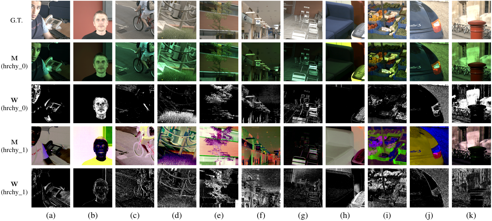
Figure 5 presents some examples to visualize how the ReWUs work and what it has learned. As expected, the ReWU connected to the input images highlights achromatic pixels with moderate brightness (subfigures a and f), the surfaces with high reflectance (subfigures g and h), as well as some memory colors with high frequency of occurrences like skin tone (subfigures a–c) and green on the plants (subfigures d, e, and i). In the other hand, ReWU also suppresses those eccentric colors that may lead to the prejudicial decisions for the illuminant estimation, for example, the red paint on the wall (subfigure b), the orange on the peppers (subfigure i), the navy blue on the roadster (subfigure j), and the scarlet on the pillar box (subfigure k). The great interpretability of the ReWU makes it possible to serve as a guidance for designing statistics-based methods, especially for those low-end devices that do not have sufficient computational capacity to run CNN-based models.
To investigate how the confidence estimation branch helps to improve the reliability of local estimates aggregation, we draw a scatterplot of the angular errors of local estimates with respect to the confidence scores for all sub-images in the MultiCam dataset, as shown in Fig. 6. As expected, the confidence estimation branch has successfully learned to assign high confidence scores for images that can be accurately estimated, and low scores for those that are prone to be erroneous. It can also be observed in Fig. 6 that some images with very low angular error (even ) are assigned with low confidence scores, which we assume is due to the loss function and the training strategy we used—the confidence estimation branch is prone to penalize those incorrectly predicted images by assigning them with low confidence socres, whilst be more “tolerant” to cases where unconfident images are actually well-predicted.
Furthermore, we sorted all the sub-images in the validation set by their confidence scores and surprisedly found that decision-making behavior of the confidence estimation branch was very similar to human’s color constancy mechanisms: when the scenes contained valuable clues for estimating illuminant color, e.g., objects with memory colors and/or recognizable patterns, the network became more confident about its estimates; oppositely, when the objects and/or colors in the scenes were difficult to identify, the network appeared ambiguous about its decisions and thus produced low confidence scores. Figure 7 demonstrates some typical sub-images from the validation set with different levels of uncertainties, in which scenes containing frequently-occurring objects (lawns, neutral surfaces, brick roofs, etc.) are categorized as “strongly confident to estimate”, and scenes with vague patterns (pseudo-neutral objects, surfaces with a dominant color, etc.) are categorized as “unconfident to estimate”.


VI Conclusion
A novel illuminant color estimation framework is proposed to exploit useful cues from feature maps in an efficient and interpretable way. To quantify the confidences of local illuminant estimates, an uncertainty prediction branch is included, upon which more flexible decisions can be made to determine the illuminant color. Experimental results indicate that the proposed method achieves comparative performance with other state-of-the-art high-level models for most of metrics with a more compact model size and lower computational burden, making it suitable for applications deployed on mobile platforms. In addition to being employed for computational color constancy, the image feature reweight unit (ReWU) also exhibits reasonable potential for other color-relevant applications such as fine-grained classification and image semantic segmentation. As the future work we plan to investigate if the confidence estimation branch could be improved so as to reduce the occurrence of “false negative” samples, i.e. images with good predictions but assigned with low confidence score, possibly by using some reinforcement learning strategy or by proposing a better loss function.
[Proof of Equation (17)]
Proof:
For the sake of briefness, let and be the random variables of values in the channel axes of and , respectively.
By definition, the distribution function for is calculated as
| (21) | ||||
where the subscripts are channel indices, is the number of channels in . Since all values in are i.i.d., we have
| (22) | ||||
According to the definition of the channel normalization in (16), approximately follows the standard normal distribution, which yields
| (23) |
where is the cumulative distribution function of the standard normal distribution. Therefore,
| (24) |
The expectation of can be calculated as
| (25) | ||||
where is the probability density function of the standard normal distribution. ∎
Acknowledgment
This research was supported by Zhejiang Province Foundation for Cultural Heritage Preservation Technology (2017010) and Fundamental Research Funds for the Central Universities (2018FZA128).
References
- [1] D. H. Brainard and B. A. Wandell, “Analysis of the retinex theory of color vision,” J. Opt. Soc. Am. A, vol. 3, no. 10, pp. 1651–1661, Oct 1986.
- [2] E. Y. Lam, “Combining gray world and retinex theory for automatic white balance in digital photography,” in Proc. IEEE International Symposium on Consumer Electronics, 2005. (ISCE 2005)., June 2005, pp. 134–139.
- [3] X. S. Zhang, S. B. Gao, R. X. Li, X. Y. Du, C. Y. Li, and Y. J. Li, “A retinal mechanism inspired color constancy model,” IEEE Trans. Image Process., vol. 25, no. 3, pp. 1219–1232, March 2016.
- [4] G. Buchsbaum, “A spatial processor model for object colour perception,” J. Franklin Inst., vol. 310, no. 1, pp. 1–26, 1980.
- [5] J. van de Weijer and T. Gevers, “Color constancy based on the grey-edge hypothesis,” in Proc. IEEE International Conference on Image Processing, vol. 2, Sept 2005, pp. II–722–5.
- [6] J. van de Weijer, T. Gevers, and A. Gijsenij, “Edge-based color constancy,” IEEE Trans. Image Process., vol. 16, no. 9, pp. 2207–2214, Sept 2007.
- [7] S. Hannah and Z. Qasim, “Colour constancy in context: Roles for local adaptation and levels of reference,” Journal of Vision, vol. 4, no. 9, p. 3, 2004.
- [8] G. D. Finlayson, S. D. Hordley, and P. M. HubeL, “Color by correlation: a simple, unifying framework for color constancy,” IEEE Trans. Pattern Anal. Mach. Intell., vol. 23, no. 11, pp. 1209–1221, Nov 2001.
- [9] K. Barnard, “Improvements to gamut mapping colour constancy algorithms,” in European conference on computer vision. Springer, 2000, pp. 390–403.
- [10] D. H. Brainard and W. T. Freeman, “Bayesian color constancy,” J. Opt. Soc. Am. A, vol. 14, no. 7, pp. 1393–1411, Jul 1997.
- [11] D. Cheng, B. Price, S. Cohen, and M. S. Brown, “Effective learning-based illuminant estimation using simple features,” in IEEE Conf. Comput. Vis. Pattern Recognit, June 2015, pp. 1000–1008.
- [12] S. Bianco, C. Cusano, and R. Schettini, “Color constancy using cnns,” in IEEE Conf. Comput. Vis. Pattern Recognit, 2015, pp. 81–89.
- [13] Y. Hu, B. Wang, and S. Lin, “Fc4: Fully convolutional color constancy with confidence-weighted pooling,” in IEEE Conf. Comput. Vis. Pattern Recognit, 2017, pp. 4085–4094.
- [14] A. Krizhevsky, I. Sutskever, and G. E. Hinton, “Imagenet classification with deep convolutional neural networks,” in Advances in neural information processing systems, 2012, pp. 1097–1105.
- [15] A. Mahmoud, “Semantic white balance: Semantic color constancy using convolutional neural network,” arXiv preprint arXiv:1802.00153, 2018.
- [16] F. N. Iandola, M. W. Moskewicz, K. Ashraf, S. Han, W. J. Dally, and K. Keutzer, “Squeezenet: Alexnet-level accuracy with 50x fewer parameters and <1mb model size,” CoRR, vol. abs/1602.07360, 2016. [Online]. Available: http://arxiv.org/abs/1602.07360
- [17] H. Kolb, “How the retina works: Much of the construction of an image takes place in the retina itself through the use of specialized neural circuits,” American scientist, vol. 91, no. 1, pp. 28–35, 2003.
- [18] L. Shi and B. Funt, “Maxrgb reconsidered,” Journal of Imaging Science and Technology, vol. 56, no. 2, pp. 20 501–1–20 501–10, 2012.
- [19] H. Joze, M. S. Drew, G. D. Finlayson, and P. Rey, “The role of bright pixels in illumination estimation,” Color and Imaging Conference, vol. 2012, no. 1, pp. 41–46, 2012.
- [20] D. Cheng, D. K. Prasad, and M. S. Brown, “Illuminant estimation for color constancy: why spatial-domain methods work and the role of the color distribution,” J. Opt. Soc. Am. A, vol. 31, no. 5, pp. 1049–1058, May 2014.
- [21] H. Lei, G. Jiang, and L. Quan, “Color constancy with derivative colors,” CoRR, vol. abs/1611.08389, 2016. [Online]. Available: http://arxiv.org/abs/1611.08389
- [22] B. K. P. Horn and R. W. Sjoberg, “Calculating the reflectance map,” Appl. Opt., vol. 18, no. 11, pp. 1770–1779, Jun 1979.
- [23] M. Lin, Q. Chen, and S. Yan, “Network in network,” arXiv preprint arXiv:1312.4400, 2013.
- [24] J. Barron and Y. T. Tsai, “Fast fourier color constancy,” in IEEE Conf. Comput. Vis. Pattern Recognit, 2017.
- [25] Y. C. Liu, W. H. Chan, and Y. Q. Chen, “Automatic white balance for digital still camera,” IEEE Trans. Consum. Electron., vol. 41, no. 3, pp. 460–466, Aug 1995.
- [26] C. C. Weng, H. Chen, and C. S. Fuh, “A novel automatic white balance method for digital still cameras,” in Proc. IEEE International Symposium on Circuits and Systems, May 2005, pp. 3801–3804 Vol. 4.
- [27] J. Huo, Y. Chang, J. Wang, and X. Wei, “Robust automatic white balance algorithm using gray color points in images,” IEEE Trans. Consum. Electron., vol. 52, no. 2, pp. 541–546, 2006.
- [28] V. Nair and G. E. Hinton, “Rectified linear units improve restricted boltzmann machines,” in ICML, 2010, pp. 807–814.
- [29] C. Szegedy, w. Liu, Y. Jia, P. Sermanet, S. Reed, D. Anguelov, D. Erhan, V. Vanhoucke, and A. Rabinovich, “Going deeper with convolutions,” in IEEE Conf. Comput. Vis. Pattern Recognit, June 2015, pp. 1–9.
- [30] X. Zhang, X. Zhou, M. Lin, and J. Sun, “Shufflenet: An extremely efficient convolutional neural network for mobile devices,” CoRR, vol. abs/1707.01083, 2017. [Online]. Available: http://arxiv.org/abs/1707.01083
- [31] T. Hui, X. Tang, and C. Loy, “Liteflownet: A lightweight convolutional neural network for optical flow estimation,” in IEEE Conf. Comput. Vis. Pattern Recognit, 2018. [Online]. Available: http://mmlab.ie.cuhk.edu.hk/projects/LiteFlowNet/
- [32] S. Bianco and R. Schettini, “Color constancy using faces,” in IEEE Conf. Comput. Vis. Pattern Recognit, 2012, pp. 65–72.
- [33] F. Wang, M. Jiang, C. Qian, S. Yang, C. Li, H. Zhang, X. Wang, and X. Tang, “Residual attention network for image classification,” CoRR, vol. abs/1704.06904, 2017. [Online]. Available: http://arxiv.org/abs/1704.06904
- [34] T. Pearce, M. Zaki, A. Brintrup, and A. Neely, “High-quality prediction intervals for deep learning: A distribution-free, ensembled approach,” arXiv preprint arXiv:1802.07167, 2018.
- [35] T. DeVries and G. W. Taylor, “Learning confidence for out-of-distribution detection in neural networks,” CoRR, vol. abs/1802.04865, 2018. [Online]. Available: https://arxiv.org/abs/1802.04865
- [36] C. Szegedy, V. Vanhoucke, S. Ioffe, J. Shlens, and Z. Wojna, “Rethinking the inception architecture for computer vision,” in IEEE Conf. Comput. Vis. Pattern Recognit, 2016, pp. 2818–2826.
- [37] S. Ioffe and C. Szegedy, “Batch normalization: Accelerating deep network training by reducing internal covariate shift,” in ICML, ser. ICML’15, 2015, pp. 448–456.
- [38] J. L. Ba, J. R. Kiros, and G. E. Hinton, “Layer normalization,” arXiv preprint arXiv:1607.06450, 2016.
- [39] A. V. D. Ulyanov and V. Lempitsky, “Instance normalization: The missing ingredient for fast stylization,” arXiv preprint arXiv:1607.08022, 2016.
- [40] Y. Wu and K. He, “Group normalization,” arXiv preprint arXiv:1803.08494, 2018.
- [41] G. Hemrit, G. Finlayson, A. Gijsenij, P. Gehler, S. Bianco, and M. Drew, “Rehabilitating the color checker dataset for illuminant estimation,” arXiv preprint arXiv:1805.12262, 2018.
- [42] L. Shi and B. Funt. Re-processed version of the gehler color constancy dataset of 568 images. [Online]. Available: http://www.cs.sfu.ca/~colour/data/
- [43] S. Bianco, C. Cusano, and R. Schettini, “Single and multiple illuminant estimation using convolutional neural networks,” IEEE Trans. Image Process., vol. 26, no. 9, pp. 4347–4362, 2017.
- [44] N. Banić and S. Lončarić, “Unsupervised learning for color constancy,” arXiv preprint arXiv:1712.00436, 2017.
- [45] D. Coffin. Decoding raw digital photos in linux. [Online]. Available: https://www.cybercom.net/~dcoffin/dcraw/
- [46] I. Fryc, S. Brown, W. Steven, and O. Yoshihiro, “Spectral matching with an led-based spectrally tunable light source,” in Fifth International Conference on Solid State Lighting, vol. 5941, 2005, p. 59411I.
- [47] “Specifications for the chromaticity of solid state lighting products,” American National Standards Institute, Standard, 2011.
- [48] M. Abadi, A. Agarwal, P. Barham, E. Brevdo, Z. Chen, C. Citro, G. S. Corrado, A. Davis, J. Dean, M. Devin, S. Ghemawat, I. Goodfellow, A. Harp, G. Irving, M. Isard, Y. Jia, R. Jozefowicz, L. Kaiser, M. Kudlur, J. Levenberg, D. Mané, R. Monga, S. Moore, D. Murray, C. Olah, M. Schuster, J. Shlens, B. Steiner, I. Sutskever, K. Talwar, P. Tucker, V. Vanhoucke, V. Vasudevan, F. Viégas, O. Vinyals, P. Warden, M. Wattenberg, M. Wicke, Y. Yu, and X. Zheng, “TensorFlow: Large-scale machine learning on heterogeneous systems,” 2015, software available from tensorflow.org. [Online]. Available: https://www.tensorflow.org/
- [49] T. Dozat, “Incorporating nesterov momentum into adam,” 2016.
- [50] N. Srivastava, G. Hinton, A. Krizhevsky, I. Sutskever, and R. Salakhutdinov, “Dropout: A simple way to prevent neural networks from overfitting,” The Journal of Machine Learning Research, vol. 1 5, no. 1, pp. 1929–1958, 2014.
- [51] W. Shi, C. L. Chen, and X. Tang, “Deep specialized network for illuminant estimation,” in European Conference on Computer Vision. Springer, 2016, pp. 371–387.
- [52] Y. H. Geoffroy, S. Kalyan, H. Sunil, G. Emiliano, and L. J. François, “Deep outdoor illumination estimation,” in IEEE Conf. Comput. Vis. Pattern Recognit, 2017.
- [53] J. T. Barron, “Convolutional color constancy,” in Proc. IEEE International Conference on Computer Vision, 2015, pp. 379–387.
- [54] G. D. Finlayson and E. Trezzi, “Shades of gray and colour constancy,” in Color and Imaging Conference, vol. 2004, no. 1. Society for Imaging Science and Technology, 2004, pp. 37–41.
- [55] P. V. Gehler, C. Rother, A. Blake, T. Minka, and T. Sharp, “Bayesian color constancy revisited,” in IEEE Conf. Comput. Vis. Pattern Recognit, June 2008, pp. 1–8.
- [56] A. Chakrabarti, K. Hirakawa, and T. Zickler, “Color constancy with spatio-spectral statistics,” IEEE Trans. Pattern Anal. Mach. Intell., 2012.
- [57] Y. Qian, K. Chen, J. Nikkanen, J. Kämäräinen, and J. Matas, “Dichromatic gray pixel for camera-agnostic color constancy,” arXiv preprint arXiv:1803.08326, 2018.
- [58] S. Bianco and C.Cusano, “Quasi-unsupervised color constancy,” in IEEE Conf. Comput. Vis. Pattern Recognit, 2019, pp. 12 212–12 221.
- [59] Y. Qian, J. Kämäräinen, J. Nikkanen, and J. Matas, “On finding gray pixels,” in IEEE Conf. Comput. Vis. Pattern Recognit, 2019, pp. 8062–8070.
![[Uncaptioned image]](1806.09248v3/Qiu.png) |
Jueqin Qiu received his B.S. degree in optical engineering from Beijing University of Aeronautics and Astronautics, China, in 2014. He is currently pursuing the Ph.D. degree in College of Optical Science and Engineering at Zhejiang University. His current research interests include computer vision, digital imaging processing, and color science. |
![[Uncaptioned image]](1806.09248v3/Xu.png) |
Haisong Xu received his Ph.D. degree in optical engineering from Zhejiang University, China, in 1993. He was a postdoctoral research fellow in Zhejiang University from 1994 to 1995 and in Chiba University, Japan, from 1999 to 2001. Now he is a professor in College of Optical Science and Engineering at Zhejiang University. His current research interests include color science, imaging technology, and lighting engineering. He is the China representative in D1 of CIE, in AIC, and in ACA. |
![[Uncaptioned image]](1806.09248v3/Ye.png) |
Zhengnan Ye received his B.S. degree in optical engineering from Zhejiang University, China, in 2015. He is now studying for the Ph.D. degree in College of Optical Science and Engineering at Zhejiang University. His research interests includes color science and multispectral imaging technology. |