Rapid computation of far-field statistics for random obstacle scattering

We shall recall the solution of the boundary value problem (1.2) by means of boundary integral equations. For the sake of simplicity in representation, we assume here that the domain $D$ is fixed with a smooth boundary $\Gamma=\partial D$.

We introduce the acoustic single layer operator

and the acoustic double layer operator

Herein, $\Phi(\cdot,\cdot)$ denotes the fundamental solution of the Helmholtz equation. It is given by

where $H_{0}^{(1)}$ denotes the zeroth order Hankel function of the first kind.

Then, if the incident wave is given by

for some direction ${\bf d}\in\mathbb{R}^{d}$, the Neumann data of the total wave $u=u_{\operatorname{inc}}+u_{\operatorname{s}}$ at the boundary $\Gamma$ can be determined by the boundary integral equation

where $\mathcal{K}^{\star}$ denotes the adjoint double-layer operator, ${\bf n}$ the outward pointing normal vector and $\eta\in\mathbb{R}\setminus\{0\}$ is chosen such that $\eta\operatorname{Re}(\kappa)>0$, see [1, 5].

From the Cauchy data of $u$ at $\Gamma$, we can determine the scattered wave $u_{\operatorname{s}}$ in any point in the exterior of the scatterer by applying the potential evaluation

By letting $\|{\bf x}\|_{2}$ tend to infinity in (2.2), we derive a closed expression for the far-field of the total wave $u$. Namely, the far-field at a point $\widehat{\bf x}\in\mathbb{S}^{1}$ is given in accordance with

Herein, the far-field kernel $\Phi_{\infty}(\cdot,\cdot)$ is given according to

We shall introduce the sphere

of radius $R>0$, being sufficiently large to guarantee that $\Sigma$ encloses the domain $D$. By differentiating (2.2), it is seen that the gradient of the scattered wave can simply be computed by

Thus, we can compute the Cauchy data of the scattered wave at the artificial interface $\Sigma$. Especially, it holds

where ${\bf n}_{\bf x}=\nicefrac{{\bf x}}{{\|{\bf x}\|_{2}}}$ is the outward pointing normal at ${\bf x}\in\Sigma$.

For any ${\bf x}\in\mathbb{R}^{d}$ with $\|{\bf x}\|_{2}>R$, we can now either use the representation formula (2.2) or the representation formula

to evaluate the scattered wave $u_{\operatorname{s}}$ at any point ${\bf x}\in\mathbb{R}^{d}$ with $\|{\bf x}\|_{2}>R$. In particular, letting $R\to\infty$, we obtain for the far-field the formula

As we will see, the major advantage of (2.4) and (2.5) over (2.2) and (2.3) in case of a random scatterer is that the sphere $\Sigma$ has a fixed shape.

We remark that an artificial interface being different from a circle can of course be chosen as well.

In this section, we introduce a description of random obstacles by means of random vector fields, as they have originally been considered in [11] in the context of the domain mapping method. To that end, let $(\Omega,\mathcal{A},\mathbb{P})$ denote a complete and separable probability space with $\sigma$-algebra $\mathcal{A}$ and probability measure $\mathbb{P}$. Here, complete means that $\mathcal{A}$ contains all $\mathbb{P}$-null sets. For a given real or complex Banach space $\mathcal{X}$, we introduce the Lebesgue-Bochner space $L_{\mathbb{P}}^{p}(\Omega;\mathcal{X})$, $1\leq p\leq\infty$, which consists of all equivalence classes of strongly measurable functions $v\colon\Omega\to\mathcal{X}$ with bounded norm

If $p=2$ and $\mathcal{X}$ is a separable Hilbert space, then the Lebesgue-Bochner space $L_{\mathbb{P}}^{p}(\Omega;\mathcal{X})$ is isomorphic to the tensor product space $L_{\mathbb{P}}^{2}(\Omega)\otimes\mathcal{X}$. For more details on Lebesgue-Bochner spaces, we refer the reader to [13].

For $p\geq 2$ and a given random field $v\in L^{p}(\Omega;\mathcal{X})$, we can introduce the expectation

and the variance

With straighforward modifications, these definitions remain valid for real valued random fields.

Now, to define the random obstacle $D(\omega)\subset\mathbb{R}^{d}$, we assume the existence of a nominal obstacle $D_{0}\subset\mathbb{R}^{d}$, with boundary $\Gamma_{0}\mathrel{\mathrel{\mathop{:}}=}\partial D_{0}$, and of a uniform $C^{1}$-diffeomorphism

i.e. there holds

such that $D(\omega)$ is implicitly given by the relation

Consequently, we obtain

Moreover, we define the hold-all domain $\mathcal{D}$ according to

Due to (3.1), it holds ${\bf V}\in L^{\infty}\big(\Omega;C^{1}(\overline{D_{0}})\big)\subset L^{2}\big(\Omega;C^{1}(\overline{D_{0}})\big)$. Hence, the vector field ${\bf V}$ can be represented by a Karhunen-Loève expansion, cf. [17], of the form

An efficient way to compute the Karhunen-Loève expansion if the mean and the covariance function of the random (vector) field under consideration are known is given by the pivoted Cholesky decomposition. This accounts particularly for random vector fields, see [9, 10, 18].

The anisotropy which is induced by the spatial parts $\{{\bf V}_{k}\}_{k}$, describing the fluctuations around the nominal value $\mathbb{E}[{\bf V}]({\bf x})$ in (3.3), is encoded by the quantities

For our modeling, we shall also make the following common assumptions.

We remark that it holds without loss of generality $\mathbb{E}[{\bf V}]({\bf x})={\bf x}$, otherwise we have to choose an appropriate reparametrization. Moreover, identifying the random variables by their image ${\bf y}\in\square\mathrel{\mathrel{\mathop{:}}=}[-1,1]^{\mathbb{N}}$, we end up with the representation

The corresponding image measure $\mu$ is given by the product of the push forward measure $\nu=\nicefrac{{\operatorname{d}\!y}}{{2}}$ according to $\mu\mathrel{\mathrel{\mathop{:}}=}\otimes_{k=1}^{\infty}\nu$. The Jacobian of ${\bf V}$ with respect to the spatial variable ${\bf x}$ is thus given by

The uniformity condition implies that the functional determinant $\det{\bf J}({\bf x},{\bf y})$ is either uniformly positive or negative, see [11] for more details. Hence, we may assume without loss of generality

for every ${\bf x}\in D_{0}$ and almost every ${\bf y}\in\square$, where $c,C>0$ are some constants. For a sufficiently fine discretization of the domain $D_{0}$, this property carries over to the finite element approximation of ${\bf V}$ and ${\bf J}$, respectively. Consequently, a quasi-uniform mesh will always be mapped to a quasi-uniform mesh by ${\bf V}$. Again, we refer to [11] for the details. Hence, under the uniformity condition (3.1) no remeshing of $D({\bf y})$ or $\Gamma({\bf y})$ is necessary for different realizations of ${\bf y}\in\square$. However, we emphasize that the discretization of ${\bf V}$ and hence the mesh for $D_{0}$ needs to be sufficiently fine in order to guarantee (3.1) also for the discretized random vector field.

In the numerical examples, we will restrict ourselves to star-like scatterers in two spatial dimensions. Especially, since we consider a boundary integral approach to solve the Helmholtz equation, we shall only define here the random vector field only for the boundary $\Gamma_{0}$.

Without loss of generality, we assume that the scatterer $D(\omega)$ is star-like with respect to the origin ${\bf 0}\in\mathbb{R}^{2}$. Then, we can represent its boundary $\Gamma({\omega})$ by a parametrization of the form

where

denotes the radial direction and radius function $r(\phi,\omega)$ is a real valued random field $r\in L^{2}\big(\Omega;C^{n}_{\text{per}}([0,2\pi])\big)$. As before, the Karhunen-Loève expansion of $r$ can be computed if $\mathbb{E}[r](\phi)$ and

are known. However, we will assume here that $r$ is of the particular form

In this case, the spatial regularity is entirely encoded in the coefficients $a_{k}$, $k\geq 0$, see [14]. By construction, the random fluctuations of the radius (3.7) are centered, i.e., their mean vanishes, and we conclude

In order to guarantee that each realization ${\bf y}\in[-1,1]^{\mathbb{N}}$ results in a boundary of a valid domain $D({\bf y})$, we shall further assume that

Moreover, it is assumed that $r_{0}\in C_{{\rm per}}^{2}([0,2\pi])$ as well as that the sequence $(a_{k})_{k}$ decays sufficiently fast to ensure $r(\cdot,{\bf y})\in C_{{\rm per}}^{2}([0,2\pi])$ for all ${\bf y}\in\square$. This for example guaranteed if $|a_{k}|\leq ck^{-(3+\varepsilon)}$ for any $\varepsilon>0$ and some constant $c>0$.

The random boundary $\Gamma({\bf y})$ is hence given by

Consequently, there holds ${\bf V}|_{\Gamma_{0}}={\boldsymbol{\gamma}}$, where $\Gamma_{0}=r_{0}{\bf e}_{r}$. In order to provide a description of the random vector field for the interior of the scatterer, which is for example needed in a domain mapping approach, a suitable extension of ${\bf V}$ to $D_{0}$ has to be defined as in e.g. [11, 14]. However, we remark that in the approach presented here, no knowledge of ${\bf V}$ inside the scatterer is required.

Now, having a suitable description of the random scatterer $D({\bf y})$ at our disposal, we can define the random scattering problem under consideration Let $u_{\operatorname{inc}}$ denote the incident wave. Then, the boundary value problem for the total field $u({\bf y})=u_{\operatorname{s}}({\bf y})+u_{\operatorname{inc}}$ for a given ${\bf y}\in\square$ reads

By the construction of $\Gamma({\bf y})$, the random scattering problem (4.1) exhibits a unique solution for each realization ${\bf y}\in\square$ of the random parameter. Moreover, it has been shown in [14] for the case of the Helmholtz transmission problem in two spatial dimensions that the total wave $u({\bf y})$ in the large wavelength regime exhibits an analytic extension with respect to the parameter ${\bf y}\in\square$ into a certain region of the complex plane. Hence, given that $\kappa$ is sufficiently small, we may employ higher order quadrature methods, like the quasi-Monte Carlo methods, see e.g. [2], or sparse quadrature methods, see e.g. [8, 14], for the computation of quantities of interest.

We can compute the scattered wave’s expectation for a given point ${\bf x}\in\mathbb{R}^{d}$ via the potential evaluation (2.2), which leads to

Of course, (4.2) makes only sense if ${\bf x}\not\in\mathcal{D}$ since otherwise there might be instances ${\bf y}\in\square$ such that ${\bf x}\in D({\bf y})$, i.e., the point ${\bf x}$ does not lie outside the scatterer almost surely, compare (3.2). In what follows, we assume that $R>0$ is chosen such that

Then, if we want to compute the expectation in many points, it is much more efficient to exploit the artificial but fixed boundary $\Sigma$ and to consider an expression similar to (2.4). However, we remark that an application of the mapping approach as in [14] is better suited if statistics of the scattered wave in the vicinity of the scatterer are of interest.

For any ${\bf x}\in\mathbb{R}^{d}$ with $\|{\bf x}\|_{2}>R$, it holds

Therefore, the scattered wave’s expectation is completely encoded in the Cauchy data at the artificial boundary $\Sigma$. This means that we only need to compute the expected Cauchy data

and

of the scattered wave at the artificial boundary $\Sigma$.

In complete analogy to (4.3), the expected far-field pattern is likewise computed by using (2.5):

The variance $\mathbb{V}[u_{\operatorname{s}}]$ of the scattered wave $u_{\operatorname{s}}$ at a point ${\bf x}\not\in B_{R}({\bf 0})$ depends nonlinearly on the Cauchy data of $u_{\operatorname{s}}$ at the artificial interface $\Sigma$. Nonetheless, we can employ the fact that the variance is the trace of the covariance function:

The covariance function is given by

and, hence,

Hence, the two-point correlation function is a higher-dimensional object. Fortunately, it depends only linearly on the second moments of the Cauchy data of the scattered wave on the artificial interface $\Sigma$, which greatly simplifies its computation. Namely, defining for ${\bf x},{\bf x}^{\prime}\in\Sigma$ the quantities

and

we have for any ${\bf x},{\bf x}^{\prime}\not\in B_{R}({\bf 0})$ the deterministic expression

As we will see in the next section, this expression can efficiently be computed if a low-rank approximation of the Cauchy datas’ correlations is available.

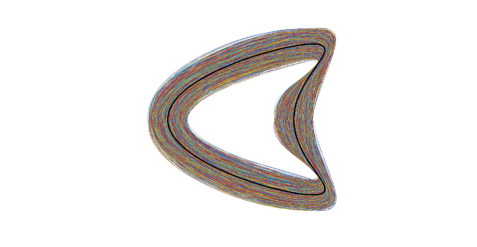
For our numerical experiments, we shall consider a kite-shaped scatterer as nominal obstacle, described by the parametrization

The random boundary is then defined in accordance with

where $\overline{\boldsymbol{\gamma}}(\phi)$ denotes the kite-shaped boundary (5.1) and $r(\phi,{\bf y})$ is given by the Fourier series

For the numerical simulation, we truncate this series after $1000$ terms.

Notice that the decay of the coefficients of the random fluctuations (5.3) are at the limit case. It would hold $r(\cdot,{\bf y})\in C_{{\rm per}}^{2}([0,2\pi])$ if the decay of the series $\{a_{k}\}_{k}$ was just a bit stronger. A visualization of $1000$ samples of this boundary is found in Figure 1.

For the numerical solution of the boundary integral equation (2.1), we apply the Nyström method to discretize the acoustic single and double layer operators. Given the parametrization (5.2) for a specific instance ${\bf y}\in[-1,1]^{1000}$, the method applies the trapezoidal rule in the $n=1000$ equidistantly distributed points $\varphi_{i}=\nicefrac{{2\pi i}}{{n}}$, $i=1,\ldots,n$, and is along the lines of [16, Chapter 12]. An appropriate desingularization technique based on trigonometric Lagrange polynomials is employed to deal with the singularities of the acoustic single and double layer operators. We remark that this method converges exponentially provided that the boundary under consideration is analytical. We refer the reader to [16, Chapter 12] for all the details.

We likewise subdivide the artificial interface $\Sigma=\partial B_{R}({\bf 0})$ by $n=1000$ equidistantly distributed points

In these points, we compute the expectations $\mathbb{E}[u_{\operatorname{s}}]({\bf z}_{j})$ and $\mathbb{E}[\nicefrac{{\partial u_{\operatorname{s}}}}{{\partial{\bf n}}}]({\bf z}_{j})$ in accordance with (4.4) and (4.5), respectively. To that end, we employ the quasi-Monte Carlo method based on $10\,000$ Halton points, cf. [19]. In [21] it is shown that this quadrature converges independent of the parameter dimension, if the derivatives with respect to the parameter ${\bf y}\in\square$ decay sufficiently fast. A thorough analysis of the computational work of the Nyström method in combination with the quasi-Monte Carlo quadrature can be found in [6].

In addition to the expectations of the Cauchy data, we compute the corresponding two-point correlation matrix

where

and

While the computation of $\mathbb{E}[u_{\operatorname{s}}]({\bf x})$ at a point ${\bf x}\not\in B_{R}({\bf 0})$ by (4.3) is straightforward, the computation of the variance $\mathbb{V}[u_{\operatorname{s}}]({\bf x})$ in accordance with (4.6) amounts to the computation of $\mathbb{C}\!\operatorname{or}[u_{\operatorname{s}}]({\bf x},{\bf x})$. This requires the approximation of the double integral over $\Sigma$. We apply again the trapezoidal rule, having thus to evaluate

The respective evaluations of the two-point correlation functions of the Cauchy data at $\Sigma$ are stored in the matrix ${\bf C}$ from (5.4). We conclude that the cost of a naive evaluation scales quadratically in the number of degrees of freedom used at the artificial interface $\Sigma$.

In order to speed-up the computations if the variance $\mathbb{V}[u_{\operatorname{s}}]({\bf x})$ has to be computed in many points, we propose to compute first a low-rank approximation of the two-point correlation function of the Cauchy data at $\Sigma$. In accordance with [9], we apply the pivoted Cholesky decomposition to get a low-rank approximation

where ${\bf L}=[\boldsymbol{\ell}_{1},\ldots,\boldsymbol{\ell}_{m}]\in\mathbb{C}^{2n\times m}$ with $m\leq n$. Note that the truncation error can rigorously be controlled in terms of the trace. Hence, the pivoted Cholesky decomposition is truncated if

for some $\varepsilon>0$. For all the details, we refer to [9, 10]. We remark that we would still end up with a separable expansion if the covariance of the Cauchy data did not admit a low-rank representation.

Having the low-rank approximation (5.5) at hand, we arrive at

Therefore, the evaluation of $\mathbb{C}\!\operatorname{or}[u_{\operatorname{s}}]({\bf x},{\bf x}^{\prime})$ requires only $\mathcal{O}(nm)$ operations instead of $\mathcal{O}(n^{2})$ operations. If $m\ll n$, this reduces the computational cost considerably, especially since $m$ depends only on the desired accuracy and thus only weakly on $n$.

References

- [1] H. Brackhage and P. Werner. über das Dirichletsche Außenraumproblem für die Helmholtzsche Schwingungsgleichung. Arch. Math., 16:325–329, 1965.
- [2] R. Caflisch. Monte Carlo and quasi-Monte Carlo methods. Acta Numer., 7:1–49, 1998.
- [3] C. Canuto and T. Kozubek. A fictitious domain approach to the numerical solution of PDEs in stochastic domains. Numerische Mathematik, 107(2):257–293, 2007.
- [4] J. E. Castrillon-Candas, F. Nobile, and R. F. Tempone. Analytic regularity and collocation approximation for elliptic {PDEs} with random domain deformations. Comput. Math. Appl., 71(6):1173–1197, 2016.
- [5] D. Colton and R. Kress. Inverse Acoustic and Electromagnetic Scattering. Springer, Berlin-Heidelberg-New York, 2 edition, 1997.
- [6] R. N. Gantner and M. D. Peters. Higher order quasi-monte carlo for baysian shape inversion. SIAM/ASA J. Uncertain. Quantif., 6(2):707–736, 2018.
- [7] L. Greengard and V. Rokhlin. A fast algorithm for particle simulations. J. Comput. Phys., 73(2):325–348, 1987.
- [8] A.-L. Haji-Ali, H. Harbrecht, M. D. Peters, and M. Siebenmorgen. Novel results for the anisotropic sparse grid quadrature. J. Complexity, 2018.
- [9] H. Harbrecht, M. Peters, and R. Schneider. On the low-rank approximation by the pivoted cholesky decomposition. Appl. Numer. Math., 62(4):428–440, 2012.
- [10] H. Harbrecht, M. Peters, and M. Siebenmorgen. Efficient approximation of random fields for numerical applications. Numer. Lin. Algebra Appl., 22:596–617, 2015.
- [11] H. Harbrecht, M. Peters, and M. Siebenmorgen. Analysis of the domain mapping method for elliptic diffusion problems on random domains. Numer. Math., 134(4):823–856, 2016.
- [12] H. Harbrecht and R. Schneider. Wavelet galerkin schemes for boundary integral equations—implementation and quadrature. SIAM J. Sci. Comput., 27(4):1347–1370, 2006.
- [13] E. Hille and R. S. Phillips. Functional analysis and semi-groups. American Mathematical Society, Providence, 1957.
- [14] R. Hiptmair, L. Scarabosio, C. Schillings, and Ch. Schwab. Large deformation shape uncertainty quantification in acoustic scattering. Adv. Comput. Math., 2018. to appear.
- [15] C. Jerez-Hanckes, Ch. Schwab, and J. Zech. Electromagnetic wave scattering by random surfaces: Shape holomorphy. Math. Models Methods Appl. Sci., 27(12):2229–2259, 2017.
- [16] R. Kress. Linear Integral Equations. Applied Mathematical Sciences 82. Springer, New York, 3 edition, 2014.
- [17] M. Loève. Probability theory I+II. Number 45 in Graduate Texts in Mathematics. Springer, New York, 4 edition, 1977.
- [18] M. D. Multerer. A note on the domain mapping method with rough diffusion coefficients. arXiv:1805.02889, 2018.
- [19] H. Niederreiter. Random Number Generation and Quasi-Monte Carlo Methods. Society for Industrial and Applied Mathematics, Philadelphia, 1992.
- [20] G. Of, O. Steinbach, and P. Urthaler. Fast evaluation of volume potentials in boundary element methods. SIAM J. Sci. Comput., 32(2):585–602, 2010.
- [21] X. Wang. A constructive approach to strong tractability using quasi-Monte Carlo algorithms. J. Complexity, 18:683–701, 2002.
- [22] D. Xiu and D. M. Tartakovsky. Numerical methods for differential equations in random domains. SIAM Journal on Scientific Computing, 28(3):1167–1185, 2006.