Computation over Wide-Band MAC: Improved Achievable Rate through Sub-Function Allocation

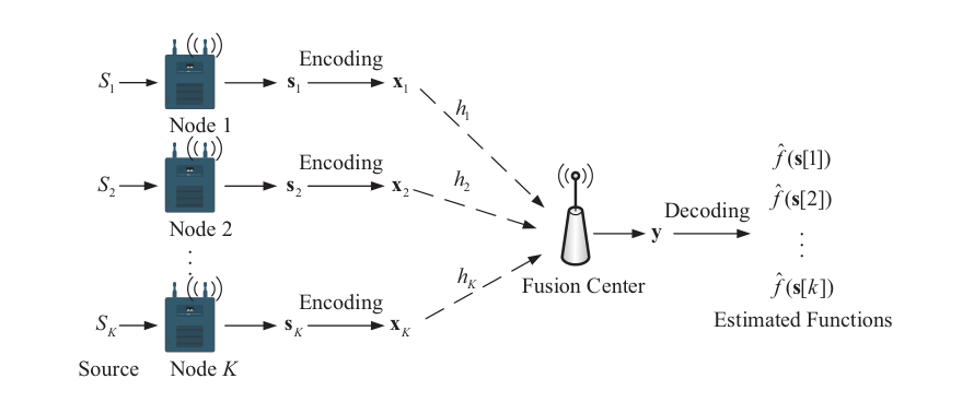
A classical framework of CoMAC is depicted in Fig. 1. In this framework, the fusion center is designed to compute a desired function from $K$ nodes. Each node obtains data from a corresponding random source for $T_{d}$ times, then giving a data vector of length $T_{d}$.

Using Definition 1, the desired function determined by the random source vector $\bm{\mathrm{s_{r}}}$ can be expressed as $f(\bm{\mathrm{s_{r}}})$, and its definition is in the following.

Definition 2 shows that the desired function $f(\bm{\mathrm{s}}[j])$ is computed by all $K$ nodes participating in the computation. In some cases, we only need to choose $M$ nodes to participate in the computation each time. Then the desired function $f(\bm{\mathrm{s}}[j])$ has to be divided into $B=\frac{K}{M}\in\mathbb{N}$ parts. The function which only uses part of the nodes is called sub-function, and its definition is given as follows.

Thus, the fusion center reconstructs the desired function based on $B$ sub-functions, when $K$ nodes are divided into $B$ parts.

In order to achieve reliable computations against noise, we apply a block code named sequences of nested lattice codes[15] throughout this paper. Based on the block coding, the definitions of encoding and decoding are given as follows.

Considering the block code with length $n$, the definition of computation rate[17, 16, 4, 19] can be given as follows.

Wide-band signal transmission has to face frequency selective fading because the coherence bandwidth of the channel is smaller than the signal bandwidth. OFDM is well-suited to provide robustness against fading. Thus, we describe a CoMAC-OFDM system with $N$ sub-carriers during $T_{s}$ OFDM symbols while the length of the block code is $n$. Then, the $m$-th received OFDM symbol at the fusion center in the frequency domain can be given by

where $T_{s}=\lceil\frac{n}{N}\rceil$, $\bm{V}_{i}=\mathrm{diag}\left\{\frac{|h_{i,1}[m]|}{h_{i,1}[m]}\sqrt{P_{i,1}[m]},\cdots,\frac{|h_{i,N}[m]|}{h_{i,N}[m]}\sqrt{P_{i,N}[m]}\right\}$ is the power allocation matrix of node $i$ where each diagonal element is the power allocated to the $g$-th sub-carrier, $\bm{H}_{i}[m]=\mathrm{diag}\left\{h_{i,1}[m],\cdots h_{i,N}[m]\right\}$ is a diagonal matrix of which the diagonal element is the frequency response of each sub-carrier for node $i$, $\bm{X}_{i}[m]=\mathrm{diag}\left\{x_{i,1}[m],x_{i,2}[m],\cdots,x_{i,N}[m]\right\}$ is the transmitted diagonal matrix of node $i$ at the $m$-th OFDM symbol, the diagonal element $x_{i,g}[m]$ in $\bm{X}_{i}[m]$ represents an element whose index is $(m-1)N+g$ in the transmitted vector $\bm{\mathrm{x}}_{i}$ (See Definition 4) for node $i$ and the diagonal element of $\bm{W}[m]$ can be regarded as identically and independently distributed (i.i.d.) complex Gaussian random noise following $\mathcal{CN}(0,\frac{1}{N})$.

According to the above expression, the received signal in the $g$-th sub-carrier at the $m$-th OFDM symbol can be expressed as

where $g\in[1:N]$, $m\in[1:T_{s}]$, $v_{i,g}[m]$ is the $g$-th diagonal element from $\bm{V}_{i}[m]$, $h_{i,g}[m]$ from $\bm{H}_{i}[m]$ is the frequency response of the $g$-th sub-carrier of node $i$ at the $m$-th OFDM symbol, $w_{i,g}[m]$ is i.i.d. complex Gaussian random noise following $\mathcal{CN}(0,\frac{1}{N})$.

The above equations assume perfect synchronization and perfect removal of inter-carrier interference.

In [16], the authors provided the computation rate for the arithmetic sum and type functions (See Remark 1) in fading MAC, i.e., the channel coefficients are i.i.d. and vary independently over time.

Unfortunately, for wireless networks with a massive number of nodes, the computation rate approaches 0 as $K$ increases, which is a vanishing computation rate. To resolve the problem, an opportunistic CoMAC system has been discussed in [17]. In each time slot, only $M$ nodes which have the largest $M$ channel gains participate in the transmission such that the indexes of the $M$ chosen nodes is in the set $\left\{\mathcal{I}_{i}\right\}_{i\in[1:M]}$.

However, the wide-band CoMAC has not been discussed and the improvement of computation rate is still limited in [17, 24, 19, 4, 16, 18, 12, 25, 26]. Therefore, Our paper focuses on designing a framework of CoMAC for wide-band transmission, which can be robust against both frequency selective fading and the vanishing computation rate. Apart from this, under our sub-function allocation and power allocation, we achieve a higher computation rate and provide a improved non-vanishing computation rate compared with the conventional CoMAC schemes.

We employ OFDM design into wide-band CoMAC and divide a desired function into $B=\frac{K}{M}\in\mathbb{N}$ sub-functions. By allocating these sub-functions into different sub-carriers, the computation rate based on CoMAC-OFDM is presented in Theorem 3.

As shown in Fig. 2, sub-function allocation includes three main parts, function division, function allocation and function reconstruction. We provide a simplified description on sub-function allocation based on CoMAC-OFDM system as follows.

• •

  Function Division. In Fig. 2a, Node $i$ gets data from the corresponding random source and obtains the data vector $\bm{\mathrm{s}}_{i}$. Then, $4$ desired functions is divided into $8$ sub-functions, which means only $2$ chosen nodes participate in the computation for a sub-function.

• •

  Function Allocation. Each sub-function is only allocated to the sub-carrier where the channel gains of the chosen nodes are the largest. For a sub-function $f(s_{1}[4],s_{4}[4])$ in Fig. 2b, the chosen nodes are Node 1 and Node 4. When the channel gains of Nodes 1 and 4 are the largest ones in the $3$-th sub-carrier at the $2$-th OFDM symbol, e.g., $\left|h_{1}\right|\geq\left|h_{4}\right|\geq\left|h_{2}\right|\geq\left|h_{3}\right|$, the sub-function $f(s_{1}[4],s_{4}[4])$ should be assigned to this sub-carrier. After function allocation, all the nodes transmit the corresponding OFDM symbols over the air.

• •

  Function Reconstruction. At the fusion center in Fig. 2c, two OFDM symbols are received, and each sub-function can be obtained in each sub-carrier. Using the $8$ received sub-functions, $4$ desired functions are reconstructed by using the relationship between the sub-functions and the desired functions.

However, the above description of sub-function allocation is ideal, and the following practical issues should be addressed.

1. i

   The order of the channel gains at each sub-carrier is random and depends on the channel realizations in practice. This means that it is important to establish the rules for sub-function allocation.

2. ii

   The above description ignores the encoding and decoding of nested lattice code. It needs employ sequences of nested lattice codes into sub-function allocation.

Further discussion on solving these issues is in Section IV-C.

In the sub-function allocation shown in Section IV-A, the fusion center computes one sub-function at a sub-carrier. Each sub-function is only allocated into the sub-carrier where the channel gains of the chosen $M$ nodes are the largest $M$ ones. The indexes of those chosen nodes are in a set $\left\{\mathcal{I}_{i}^{g}[m]\right\}_{i=1}^{M}$ for the $g$-th sub-carrier at the $m$-th OFDM symbol. For the sake of fairness, we assume the bandwidth of CoMAC-OFDM with N sub-carriers is the same as the bandwidth of the conventional CoMAC system which uses single carrier for transmission. It means the bandwidth of the sub-carrier is $\frac{1}{N}$ of the bandwidth of the single carrier. Then, the computation rate of a sub-function at the $m$-th OFDM symbol can be given as follows.

Only $M$ nodes are chosen from all $K$ nodes for a sub-function, which means there need be $B=\frac{K}{M}$ sub-functions to reconstruct a desired function. $\tau$ denotes a set where the elements are the indexes of the $M$ chosen nodes for a sub-function $f\left(\left\{s_{i}[j]\right\}_{i\in\tau}\right)$ (See Definition 3). Then, the set

includes all the possible sub-functions¹¹ 1 For easy presentation, we use the element $\tau\in\mathcal{S}$ stands for the sub-function $f\left(\left\{s_{i}[j]\right\}_{i\in\tau}\right)$ which is computed by these nodes in $\tau$., and the cardinality of $\mathcal{S}$ is $\left|\mathcal{S}\right|=\left({}_{M}^{K}\right)$. According to Definition 3, the sub-functions can be reconstructed into the desired function if and only if $\bigcup_{u=1}^{B}\tau_{u}=[1:K]$ and $\tau_{u}\bigcap\tau_{v}=\emptyset$ for all $u,v\in[1:B]$ and $\tau_{u},\tau_{v}\in\mathcal{S}$. We define

which contains all possible combinations that can be used to reconstruct the desired function, and $\left|\mathcal{Q}\right|=\prod_{l=0}^{B-1}\left({}_{M}^{K-Ml}\right)$.

Under our design, the length-$n$ block code is transmitted through $T_{s}$ OFDM symbols. In order to simplify the derivation, the number of OFDM symbols $T_{s}=\frac{n}{N}$ instead of $\lceil\frac{n}{N}\rceil$ in Eq. (4), which means the number of all the sub-carriers during $T_{s}$ OFDM symbols is $n$. Based on sub-function allocation, all the sub-carriers should be assigned to every sub-function. The set $\mathcal{M}_{\tau}$ for all $\tau\in\mathcal{S}$ includes those sub-carriers are assigned to sub-function $\tau$. And let a set $\mathcal{M}_{\rho}^{\tau}$ include the sub-carriers that are from $\mathcal{M}_{\tau}$ and allocated in the combination $\rho\in\mathcal{Q}$ that contains the corresponding sub-function $\tau$.

As mentioned in Issue i, Section IV-A, the order of the indexes for $K$ nodes in each sub-carrier is random depending on channel realizations in practice. It means the number of the sub-carriers in $\mathcal{M}_{\tau}$ is random. Thus, we use the following lemma to characterize the the minimum deterministic values of $\left|\mathcal{M}_{\tau}\right|$ and $\left|\mathcal{M}_{\rho}^{\tau}\right|$.

Based on sub-function allocation discussed in Section IV-A, we proposed a power allocation method with average power constraint.

Because only $M$ nodes participate in computing a sub-function in each sub-carrier depending on Theorem 3, let $P_{i,g}[m]$ represent the transmitted power in $g$-th sub-carrier at the $m$-th OFDM symbol for the node $i$, which can be given as

In order to compare it with the conventional CoMAC which uses the single carrier to transmit signal in a fair way, we assume the bandwidth of OFDM symbols with $N$ sub-carriers is the same as the bandwidth of the conventional single carrier symbols. Then, a complete OFDM symbol should use $N$ time slots to be transmitted while the number of transmitted symbols should be $N$ in the single carrier system. Hence, the average power in the $g$-th sub-carrier at the $m$-th OFDM symbol is $\mathsf{E}[x_{i,g}[m]]=\frac{P}{N}$. From

with $\mathsf{E}[x_{i,g}[m]]\leq\frac{P}{N}$, we can calculate $c$ and set

We further put $P_{\mathcal{I}_{i}^{g}[m],g}[m]$ from Eq. (26) into Eq. (8) in Theorem 3, the computation rate for CoMAC-OFDM with sub-carrier loading scheme can be written as

where the condition $(a)$ follows because the channel gains in different sub-carriers are i.i.d. random variables. In conclusion, Eq. (27) is achievable as $T_{s}$ increases (See Theorem 3), which completes the proof of Corollary 2. Particularly, Corollary 1 can be proved by setting $M=K$, which means each sub-carrier is allocated a desired function.

Based on the above analysis, we demonstrate the computation rate based on CoMAC-OFDM in Section IV-C. We further find that the computation rate using on the average power constraint for each node in each sub-carrier is not optimal. Therefore, we consider the optimal power allocation for CoMAC-OFDM, discuss an optimization problem and propose an algorithm called sponge-squeezing based on the solution.

References

- [1] G. Fettweis and S. Alamouti, “5G: Personal mobile internet beyond what cellular did to telephony,” IEEE Commun. Mag., vol. 52, no. 2, pp. 140–145, 2014.
- [2] A. Al-Fuqaha, M. Guizani, M. Mohammadi, M. Aledhari, and M. Ayyash, “Internet of things: A survey on enabling technologies, protocols, and applications,” IEEE Commun. Surv. Tutorials, vol. 17, no. 4, pp. 2347–2376, 2015.
- [3] A. Gupta and R. K. Jha, “A survey of 5G network: Architecture and emerging technologies,” IEEE access, vol. 3, pp. 1206–1232, 2015.
- [4] M. Goldenbaum, H. Boche, and S. Stańczak, “Nomographic functions: Efficient computation in clustered Gaussian sensor networks,” IEEE Trans. Wireless Commun., vol. 14, no. 4, pp. 2093–2105, 2015.
- [5] M. Goldenbaum and S. Stanczak, “Robust analog function computation via wireless multiple-access channels,” IEEE Trans. Commun., vol. 61, no. 9, pp. 3863–3877, 2013.
- [6] O. Abari, H. Rahul, and D. Katabi, “Over-the-air function computation in sensor networks,” arXiv preprint arXiv:1612.02307, 2016.
- [7] M. Goldenbaum and S. Stanczak, “On the channel estimation effort for analog computation over wireless multiple-access channels,” IEEE Wireless Commun. Lett., vol. 3, no. 3, pp. 261–264, 2014.
- [8] A. Kortke, M. Goldenbaum, and S. Stańczak, “Analog computation over the wireless channel: A proof of concept,” in SENSORS, 2014 IEEE. IEEE, 2014, pp. 1224–1227.
- [9] G. Zhu, L. Chen, and K. Huang, “Over-the-air computation in MIMO multi-access channels: Beamforming and channel feedback,” arXiv preprint arXiv:1803.11129, 2018.
- [10] L. Chen, N. Zhao, Y. Chen, F. R. Yu, and G. Wei, “Over-the-air computation for IoT networks: Computing multiple functions with antenna arrays,” IEEE IoT J., 2018, to be published, DOI 10.1109/JIOT.2018.2843321.
- [11] B. Nazer and M. Gastpar, “Computation over multiple-access channels,” IEEE Trans. Inf. Theory, vol. 53, no. 10, pp. 3498–3516, 2007.
- [12] R. Appuswamy and M. Franceschetti, “Computing linear functions by linear coding over networks,” IEEE Trans. Inf. Theory, vol. 60, no. 1, pp. 422–431, 2014.
- [13] U. Erez, S. Litsyn, and R. Zamir, “Lattices which are good for (almost) everything,” IEEE Trans. Inf. Theory, vol. 51, no. 10, pp. 3401–3416, 2005.
- [14] L. Chen, X. Qin, and G. Wei, “A uniform-forcing transceiver design for over-the-air function computation,” IEEE Wireless Commun. Lett., 2018, to appear, DOI: 10.1109/LWC.2018.2840157.
- [15] B. Nazer and M. Gastpar, “Compute-and-forward: Harnessing interference through structured codes,” IEEE Trans. Inf. Theory, vol. 57, no. 10, pp. 6463–6486, 2011.
- [16] S.-W. Jeon, C.-Y. Wang, and M. Gastpar, “Computation over Gaussian networks with orthogonal components,” IEEE Trans. Inf. Theory, vol. 60, no. 12, pp. 7841–7861, 2014.
- [17] S. W. Jeon and C. J. Bang, “Opportunistic function computation for wireless sensor networks,” IEEE Trans. Wireless Commun., vol. 15, no. 6, pp. 4045–4059, 2016.
- [18] C.-Y. Wang, S.-W. Jeon, and M. Gastpar, “Interactive computation of type-threshold functions in collocated Gaussian networks,” IEEE Trans. Inf. Theory, vol. 61, no. 9, pp. 4765–4775, 2015.
- [19] M. Goldenbaum, “Computation of real-valued functions over the channel in wireless sensor networks,” Ph.D. dissertation, Technische Universität München, 2014.
- [20] D. Tse and P. Viswanath, Fundamentals of wireless communication. Cambridge university press, 2005.
- [21] Z. Hasan, G. Bansal, E. Hossain, and V. K. Bhargava, “Energy-efficient power allocation in OFDM-based cognitive radio systems: A risk-return model,” IEEE Trans. Wireless Commun., vol. 8, no. 12, 2009.
- [22] C. Mohanram and S. Bhashyam, “Joint subcarrier and power allocation in channel-aware queue-aware scheduling for multiuser OFDM,” IEEE Trans. Wireless Commun., vol. 6, no. 9, 2007.
- [23] Y.-F. Chen and J.-W. Chen, “A fast subcarrier, bit, and power allocation algorithm for multiuser OFDM-based systems,” IEEE Trans. Veh. Technol., vol. 57, no. 2, pp. 873–881, 2008.
- [24] A. Giridhar and P. R. Kumar, “Computing and communicating functions over sensor networks,” IEEE J. Sel. Areas Commun., vol. 23, no. 4, pp. 755–764, 2005.
- [25] J. Zhan, S. Y. Park, M. Gastpar, and A. Sahai, “Linear function computation in networks: Duality and constant gap results,” IEEE J. Sel. Areas Commun., vol. 31, no. 4, pp. 620–638, 2013.
- [26] N. Ma, P. Ishwar, and P. Gupta, “Interactive source coding for function computation in collocated networks,” IEEE Trans. Inf. Theory, vol. 58, no. 7, pp. 4289–4305, 2012.
- [27] I. Csiszar and J. Körner, Information Theory: Coding Theorems for Discrete Memoryless Systems. Cambridge University Press, 2011.