Quantum Kitchen Sinks: An algorithm for machine learning on near-term quantum computers

Interest in adapting or developing machine learning algorithms for near-term quantum computers has grown rapidly. While quantum machine learning (QML) algorithms offering exponential speed-ups on universal quantum computers have been known for some time [1, 2, 3, 4, 5, 6, 7], recent interest has increasingly focused on algorithms for noisy, intermediate-scale quantum (NISQ) computers [8, 9, 10, 11, 12]. These algorithms aim to minimize the complexity of the required quantum circuit so that they may be executed by NISQ devices while still yielding meaningful results. This is in contrast to approaches that allow for arbitrarily large circuits of width and depth that grow polynomially in the input size. These approaches can only yield meaningful answers if errors are suppressed to rates that are inversely proportional to the circuit size, something that is not possible with NISQ devices and requires fault tolerance [13, 14, 15].

Many of the proposed approaches use a so-called hybrid model for NISQ computing, where the quantum processor is considered an expensive resource and is extensively supported by classical computing resources. In particular, many of these proposals use a variational approach, where parameters of a small quantum circuit are optimized using classical optimization algorithms which use measurement outcomes to compute a cost function [16, 17, 18, 19, 20, 21, 11]. While these closed-loop hybrid approaches move the computational cost of the optimization algorithm off of the quantum hardware, the iterative nature of the optimization process still requires a large number of calls to the “expensive” quantum resource.

In this paper, we propose a QML algorithm that eliminates the need for costly parameter optimization of quantum circuits. This novel open-loop hybrid algorithm, which we call quantum kitchen sinks (QKS), is inspired by a technique known as random kitchen sinks whereby random nonlinear transformations can greatly simplify the optimization of machine-learning (ML) tasks [22, 23, 24]. The general idea of QKS is to randomly sample from a family of quantum circuits and use each circuit to realize a nonlinear transformation of the input data to a measured bitstring. Subsequently, the concatenated results are processed with a classical machine learning (ML) algorithm. This approach is simple, flexible, and allows us to demonstrate that even small quantum circuits, deep in the NISQ regime, can provide significant “lift” for complex ML tasks such as the classification of hand-written digits. We further relate our circuits to common tools in ML known as kernels.

The objective in supervised ML is to approximate some a priori unknown function $f(\bm{u})$. For example, this function may be a map from images, represented by the variable $\bm{u}$, to labels, such as “cat” and “dog”. This is often done by optimizing a parameterized function $g(\bm{u};\bm{\theta})$ to maximize performance on a training set consisting of $M$ examples $\{y_{i,\text{train}},\mathbf{u}_{i,\text{train}}\}$ such that $g(\mathbf{u}_{i,\text{train}};\bm{\theta})\approx y_{i,\text{train}}$ for as many examples in the training set as possible. The quality of the approximation is often further quantified by how well $g$ performs on some test set that is different from the training set ¹¹ 1 The use of a test set helps to avoid so-called “overfitting” of $g$ to the training set, as one would like an approximation to $f$ that generalizes well to previously unseen data, not simply an approximation that works only on the training set.. A choice for $g$ that performs particularly well is a deep neural network, which is a parametrized composition of many simple nonlinear functions, such as sigmoid functions or rectified linear units [26]. Finding the parameters of $g$ that optimize performance (a process that for deep neural networks is known as deep learning) can be resource intensive, requiring large training sets and computational power [26].

Rahimi and Recht [22, 23, 24] observed that the costly optimization of the training process could be replaced by randomization. In an approach dubbed random kitchen sinks (RKS) [22, 23, 24], they showed it was possible to represent $g$ as a weighted, linear sum of simple nonlinear functions that each have random parameters. Each term in this sum is called a “kitchen sink”. The weights of the sum still need to be optimized, but this is a linear problem and, therefore, easy to solve. It has been shown that, for example, the cosine, sign (i.e., $d|x|/dx$), and indicator functions can be used to obtain good function approximations [22]. The RKS idea originated from an attempt to approximate the “kernel trick” [27, 28], by randomly sampling eigenfunctions of an integration kernel. Since then, this technique has been shown to apply beyond the sampling of a kernel, and to deliver performance that is comparable to deep learning, while relying on much simpler numerical techniques [29, 30].

The performance of the algorithm is dependent on the number of kitchen sinks $D$, the choice of nonlinear function, and the number of training examples $M$. Rahimi and Recht showed the approximation error of $g$ in RKS scales as $O(\frac{1}{\sqrt{D}}+\frac{1}{\sqrt{M}})$ [24] such that it may be necessary to have large training sets and to generate many RKS in order to achieve the same error rate as standard kernel methods ²² 2 This means, in particular, that if the kernel corresponding to a circuit Ansatz is known, it is possible to estimate the RKS error rate for that Ansatz by using a classical kernel machine, although performance as a function of $D$ is often better than what would be expected from these bounds [30]..

Before discussing how to generalize RKS to a quantum setting, we would like to make an important observation. In proposing an ML algorithm for quantum computers, there is a danger that the quantum processor will not contribute in a meaningful way to the power of the technique. If the external classical part is powerful enough, the algorithm may work in spite of the transformation made by the quantum processor. This can be seen as the flip-side of the RKS result we adapt: generic nonlinearities in the classical processing can add power to the ML algorithm, even if the quantum processing does not. For this reason, it is important in a research context that the classical portion of the algorithm be as simple and linear as possible. For this reason, we will require all classical pre- and postprocessing to be strictly linear, and consider only the added power of a nonlinear transformation enabled by the quantum processor. We will refer to this as the Linear Baseline (LB) Rule.

Applying the LB Rule to our strategy for testing and validation, we design an algorithm such that the quantum processor can be removed and the input data can be passed directly through the remaining (linear) classical part of the algorithm. We can then benchmark the performance lift provided by the quantum processor against the performance of the classical algorithm on its own. Note that a lift provided by the quantum processor in this context does not imply an absolute quantum advantage, but it does gives us a simple, operational method to identify the power added by the quantum circuit.

We now describe our approach to translate the RKS framework into something that may be computed by a quantum computer—what we call QKS (see Fig. 1).

As noted above, one of the nonlinear functions used to build RKSs is a cosine. We can easily generate cosine transformations in a quantum setting by applying a Rabi rotation to a single qubit with a rate and phase that is chosen at random, but a time duration that is a function of the input data. While this quantum construction of RKSs works well, it can easily be simulated on a classical computer.

In order to generalize this to circuits that are harder to simulate, our first step is to specify the input data encoding in more detail. We choose to encode the data into angles of rotations in the quantum circuit, while keeping the state preparation and measurement fixed (a similar approach was taken in [11] for a different QML technique). This naturally leads the measurement statistics to depend nonlinearly on the classical data.

Under the LB rule, we require that the mapping from data to angles be linear. To define a linear encoding, let $\mathbf{u}_{i}\in\mathbb{R}^{p}$ for $i=1,\ldots,M$ be a $p$-dimensional input vector from a data set containing $M$ examples. We can encode this input vector into $q$ gate parameters using a $(q\times p)$-dimensional matrix $\mathbf{\Omega}_{e}$ of the form $\mathbf{\Omega}_{e}=(\mathbf{\omega}_{1},\ldots,\mathbf{\omega}_{q})^{\intercal}$ where $\mathbf{\omega}_{k}$ is a $p$-dimensional vector with a number $r\leq p$ elements being random values and the other elements being exactly zero. We can also specify a random $q$-dimensional bias vector $\boldsymbol{\beta}_{e}$. We then get our set of random parameters $\bm{\theta}_{i,e}$ from the linear transformation $\bm{\theta}_{i,e}=\mathbf{\Omega}_{e}\mathbf{u}_{i}+\boldsymbol{\beta}_{e}$. Notice the additional index $e$ which denotes the $e$^th episode, i.e., the $e$^th repetition of the circuit parameterized through the encoding $\mathbf{\Omega}_{e},\boldsymbol{\beta}_{e}$ (see below for a discussion about episodes).

By specifying different elements of $\mathbf{\omega}_{k}$ to be nonzero, we can specify different encodings. For instance, we can encode a $p$-dimensional input vector into a single-qubit circuit by choosing $q=1$ and $r=p$. In this single-qubit encoding, all dimensions of $\mathbf{u}_{i}$ are combined into a single control parameter. Conversely, we could use a split encoding with $q=p$ and $r=1$, where each dimension of $\mathbf{u}_{i}$ is fed into a distinct control parameter. We discuss other possibilities below. Note that the set of encoding parameters $\{\mathbf{\Omega}_{e},\boldsymbol{\beta}_{e}\}_{e=1}^{E}$ is only drawn once and becomes a static part of the machine, which is used for both training and testing. For the results presented in this paper, the nonzero elements of $\mathbf{\Omega}_{e}$ are drawn from a zero-mean normal distribution with variance $\sigma^{2}$, i.e., $\mathcal{N}(0,\sigma^{2})$ and the elements of $\boldsymbol{\beta}_{e}$ are drawn from a uniform distribution $\mathcal{U}(0,2\pi)$ ³³ 3 Note that the hyperparameter $\sigma$ must be optimized during training.. However, other distributions may also be considered. These choices only partially determine the encoding. The exact structure of the circuit and how the parameters $\mathbf{\omega}_{k}$ parameterize the circuit will also have an impact on the performance of the algorithm, and illustrate the large flexibility available for designing QKSs tailored to particular datasets and applications.

The choice of distributions and the parameterization of the circuit together implicitly define a kernel which allows for QKSs to be analyzed as a standard kernel machine, as we describe later. The computation of the kernel is not necessary for the use of the QKS, and in fact may require exponentially large resources, but it may be helpful in designing the circuit Ansätze.

Once we have encoded the data into control parameters, we are ready to preprocess the data. Since the input data is encoded in circuit parameters, the choice of input state is somewhat arbitrary. For simplicity and without loss of generality, we choose the all-zeros state $\ket{\Psi_{\text{in}}}=\ket{00\ldots}$. Since any other input state would be generated by another quantum circuit, the composition of this circuit with the QKS encoding would correspond to a different circuit Ansatz.

In order to postprocess the QKS output, we must also extract classical data from the state. This is done by simply measuring the state in the computational basis—again, without loss of generality, since a basis transformation would simply translate into changing the circuit Ansatz. The output of the measurements gives us classical bits. We have some design freedom in choosing how to (classically) process these output bits into features. Under the LB rule, care should be taken in this choice such that nonlinear postprocessing is avoided. For this work, we will simply “stack” all of the bits into a $q$-dimensional feature vector.

Contrary to the RKS approach, this feature mapping is stochastic. Our proposal does not preclude averaging over many shots of the same circuit, but the numerical studies described here use only individual shots of each circuit.

Once we have constructed our feature vectors, they are fed into a classical machine learning algorithm, which under the LB rule, we take to be linear (as is also the case in RKS).

It is well-known in machine learning that transforming data into a higher-dimensional feature space can be useful. There are two strategies to generate higher-dimensional features using QKS: entangling more and more qubits, or generating more and more random circuits. The first strategy leads straightforwardly to a quantum advantage argument if the parameterized circuits used are hard to simulate [33, 34, 35, 36]. However, large, monolithic circuits may also require very low error rates. The second strategy is more readily scaled in NISQ devices, and it simply requires running $E$ fixed circuits, which we call episodes, to obtain a feature vector that is $(E\times q)$-dimensional for $q$ qubits. We expect $D$ parameters in RKS should be roughly equivalent to $E\times q$ parameters in QKS, but we do not have formal results that guarantee this correspondence.

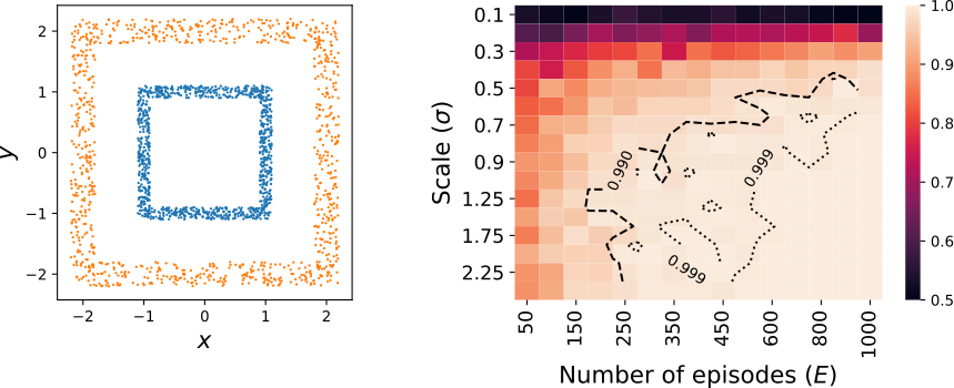
As an example to demonstrate the effectiveness of QKS, we incorporate it into a standard binary classification problem. As our classical, linear baseline, we use the logistic regression (LR) classifier provided by the scikit-learn package. As a first data set, we choose the synthetic “picture frames” dataset shown in Fig. 3. The dataset was chosen to have two classes that are not separable by a linear boundary. The training set contained $M=1600$ two-dimensional points, $800$ for each class. The classification accuracy was tested using a different set of $400$ points arranged in a similar configuration.

We coded the algorithm using the pyQuil^® Python package [37, 38] and executed it on the Rigetti QVM™, available through the Forest platform [39]. The QVM is a high-performance quantum simulator written in ANSI Common Lisp [40]. In order to run the numerical experiments in conjunction with post-processing software in Python, the QVM was extended with a new entry-point to allow high-speed execution of a large number of episodes (on the order of $10^{4}$) for a given circuit Ansatz and input $\mathbf{u}$. In particular, the QVM was extended so that a template Quil [38] program defined with the DEFCIRCUIT facility could be supplied along with a collection of DEFCIRCUIT parameter tuples. The QVM reads these parameter tuples, fills them into the supplied program in constant time, and executes the resulting program, all while eliminating unnecessary memory access and allocations. This modification to the QVM was made possible using Quil’s hybrid classical/quantum memory model. See the Appendix (e.g., Fig. 8) for examples of circuit Ansätze written in Quil.

Applying the baseline LR algorithm to the picture frame dataset yielded a classification accuracy of approximately $50\%$, meaning it performs no better than randomly assigning classes to each point. We then used the QKS construction, using the circuit shown in Fig. 2. For the data presented here, we used split encoding (defined above) with $q=p=2$ and $r=1$, and optimized over the number of episodes $E$ and the parameter $\sigma$ used in the random encoding. The best classification accuracy achieved was $>99.9\%$, a remarkable performance lift over the linear baseline, illustrating the power of QKS (see Fig. 3).

While this synthetic example illustrates the computational power provided by the QKS, it is interesting to consider a less structured classification problem originating in the real world: discriminating hand-written digits from the MNIST dataset [41]. This dataset is a well-known benchmark in machine learning. While it is a multiclass problem, we choose to focus on classifying two digits that are difficult to distinguishing using LR: “3” and “5”. The classification accuracy we obtain with LR is $95.9\%$, which will serve as our linear baseline.

The MNIST dataset has a much higher dimensionality than the previous example. Each digit is a $(28\times 28)$-pixel 8-bit grayscale image, so care must be taken to encode the data into a small number of qubits. A standard first step is to vectorize the image, by stacking the columns of the image into a $p=784$ dimensional vector. We use a slightly modified approach intended to preserve more of the spatial structure of the image. After standardizing the image ⁴⁴ 4 Standardization or $z$-normalization of a set $X\subset\mathbb{R}$ is the pointwise map $x\mapsto(x-\mathrm{E}[X])/\operatorname{Var}(X)^{2}$., to run MNIST on a $q$-qubit processor, we first split each image into $q$ rectangular tiles, and construct fixed-depth circuit Ansätze where only single-qubit gates have parameterized rotations (see Fig. 4). The encoding vectors $\mathbf{\omega}_{k}$ are then chosen to have blocks of $r=p/q$ nonzero elements that select out values of only one tile per gate parameter.

With this encoding, we have simulated the performance of QKS on the $(3,5)$-MNIST dataset for different numbers of qubits. The best error rate is $1.4\%$, which is a reduction of the error rate by more than a factor of 2 compared to the linear baseline.

In Fig. 5 we plot the minimum error rate for classifying the $(3,5)$-MNIST dataset using QKS for different numbers of qubits. Each point corresponds to the minimum error observed after optimizing the hyperparameters $\sigma$ and $E$, much like what is shown in Fig. 3. The maximum number of episodes used was 20,000. Comparing the results for different numbers of qubits, there is a clear minimum in the error rate in the range 2 to 4 qubits. For more qubits, the error rate increases again. There are a number of possible explanations for this behavior. One possibility is simply that the particular circuits chosen (including the $\mathsf{CNOT}$ networks) may be suboptimal for this task. Another possibility is that the MNIST data set is insufficiently large to properly train the larger number of parameters in the larger circuits, leading to overfitting. These and other hypotheses will be explored in future work.

It is also important to point out that quantum coherence does not play a role in “single layer” circuits, as the same output mapping can be implemented using purely classical stochastic processes (i.e., the circuits are efficiently simulatable, in the weak sense [43]). We are able to show, however, that by increasing the number of layers of the circuit Ansätze (each layer using independently chosen linear encodings) we are able to maintain similar performance (see Fig. 5). One may also consider other Ansätze based on circuits that are conjectured to be hard to simulate [33, 34, 35, 36].

A powerful feature of QKS is that specifying the form of $\mathbf{\Omega}$ allows a form of built-in compression, enabling us to classify full-sized MNIST images on small circuits. To further demonstrate this power and flexibility, we ran the classification problems we discussed here—picture frames and the (3,5) subset of MNIST—on one and two qubit circuits using a Rigetti QPU, i.e., on real quantum hardware. To our knowledge this is this is the first time image classification of MNIST images has been performed on a quantum computer.

These experiments were run on a device with 8 qubits arranged in a loop [44, 45]. The $\mathsf{CNOT}$ gate was implemented as a $\mathsf{CZ}$ operation that native to our architecture [46], preceded and followed by Hadamard operations on one of the qubits [47]. Average gate fidelities [48] for the CZ gate varied between 81% and 91% for the duration of these experiments, which ranged from 1.5h for the picture frames, to 12h and 34h for the 1 and qubit ansatze applied to the (3,5)-MNIST dataset (gates were not recalibrated during the experiments, only between them). Different episodes were measured at a rate of roughly 400 Hz, which is largely a consequence of the choice to take a single of each episode for the feature generation (much higher rates can be obtained for multiple shots of a fixed circuit, but that feature is not exploited here).

Using the 2 qubit ansatz from Fig. 2(a) on the picture frame data set, with 1000 episodes and $\sigma=1.0$, we achieved 100% accuracy on a test set of 400 examples and training set of 1600 examples, even in the presence of relatively noisy entangling gates.

We considered both the 1 qubit and the 2 qubit ansatze for the (3,5)-MNIST dataset (see the Appendix for details of the 1 qubit circuit). We did not use larger ansatze due to the connectivity limitations of the device used. We used 50% of the MNIST dataset, and did not optimize the hyperparameters using the experimental setup, using instead simulations with the QVM to choose the hyperparameters. The motivation for these choices was to reduce the runtime of the experiment. The experimental results are shown, along with the simulation results, in Fig. 5. For a one qubit circuit with $\sigma=0.05$ and $E=10,000$, we find an error rate of $3.3\%$. Even for this simplest circuit, we find QKS provides a performance lift over a linear suport vector machine. Although, the error rate is somewhat higher than the best QVM result, it compares remarkably well to the one qubit QVM result with the same hyperparamters, which is an error rate of $3.2\%$. Implementing the two qubit $\mathsf{CNOT}$ circuit shown in Fig 2 with $\sigma=0.05$ and $E=8,900$, we find an error rate of $3.7\%$. Again, this shows a clear lift despite the use of real, noisy quantum hardware.

The random sampling of nonlinear feature maps across different episodes can be connected to the use of an implicit kernel function [22, 23, 24]. Formally, the kernel is the inner product between input vectors after their nonlinear mapping by the kitchen sinks. Informally, the kernel function $k(\mathbf{u},\mathbf{v})$ of two input vectors $\mathbf{u}$ and $\mathbf{v}$ expresses the similarity between these inputs. Even though the random and quantum kitchen sinks do not explicitly use the kernel, it is instructive to calculate the implicit kernel associated with our circuits, as it can point to better ways to build circuit Ansätze, and consider the effect of noise.

We compute the implicit kernel by evaluating the inner product of two binary feature vectors sampled using a QKS circuit. Let $\mathbf{b}_{e,\mathbf{u}}(\boldsymbol{\theta}_{e})$ and $\mathbf{b}_{e,\mathbf{v}}(\boldsymbol{\theta}_{e})$ denote the vectorized output of a single episode $e$ with the random parameters $\boldsymbol{\theta}_{e}$ on the inputs $\mathbf{u}$ and $\mathbf{v}$. The inner product of the total feature vector can then be computed as

where we have added the normalization by $E$.

The quantities $\mathbf{b}_{e,\mathbf{v}}(\mathbf{\theta}_{e})$ are random variables with bit-string values $z\in\{0,1\}^{q}$. The probability of a given outcome $z$ is $p_{e,\mathbf{u}}^{(z)}=\left|\bra{z}U(\mathbf{u},\mathbf{\theta}_{e})\ket{\Psi_{\text{in}}}\right|^{2}$ where $U(\mathbf{u},\mathbf{\theta}_{e})$ is the unitary transformation realized by the QKS circuit. We then find

where the matrix $\mathbf{S}$ contains the inner product of the bit strings $z$ and $z^{\prime}$, and the vector $\mathbf{p}_{e,\mathbf{u}}$ the outcome probabilities, both indexed by $z$.

We now note that since the parameters $\boldsymbol{\theta}_{e}$ are drawn from a classical probability distribution $P(\boldsymbol{\theta})$, we can view the sum $\tilde{k}(u,v)$ as a Monte Carlo estimator. In the limit of an infinite number of episodes ($E\rightarrow\infty$), the kernel then approaches the form

Using this result, we can, for instance, calculate the implicit kernel for the circuit in Fig. 2(a). To do so, we specify that the values of the matrix $\Omega$ are drawn from a normal distribution $\mathcal{N}(0,\sigma^{2})$ and that the elements of the bias vector $\boldsymbol{\beta}_{e}$ are drawn from a uniform distribution $\mathcal{U}(0,2\pi)$. Using (1), we then find the implicit kernel as

where ${\bf u}^{(i)}$ (${\bf v}^{(i)}$) is the $i$^th tile (out of 2) of the input data vector $\mathbf{u}$ ($\mathbf{v}$) ⁵⁵ 5 For the picture frame data set, this is just the $i$^th vector component.. We see that the last term here is a radial basis function (RBF) kernel that is standard in machine learning. There are additional components, including a constant term. The second term depends only on part of the data. Similar calculations can be performed for the other circuit Ansätze, and again we find multiple terms that depend on different subsets of the data. One can imagine optimizing the $\mathsf{CNOT}$ network to maximize sensitivity to the most relevant subsets of the data, but we do not explore the possibility here.

Interestingly enough, not all circuit Ansätze lead to a useful kernel. For instance, circuit Fig. 2(b) seems similar to the just-analyzed circuit. However, if we calculate the implied kernel of this circuit, we find the constant function $k(\mathbf{u},\mathbf{v})=1/2$, independent of the input vectors $\mathbf{u}$ and $\mathbf{v}$. This suggests that this circuit should have no discrimination power and, in fact, our numerical results confirm this.

We see that QKS provides a rich structure to construct implicit kernels, with not only the choice of circuit, but the choice of encoding, choice of decoding, and choice of probability distributions shaping the kernel in understandable ways.

For context, we can compare our experimental MNIST results to simulation results based on other algorithms. For instance, ref. [12] simulates the same $(3,5)$-MNIST classification problem, using images downsampled to $8\times 8$ pixels on much wider and deeper networks. Even with noiseless circuits, they achieve an error rate of only $12.4\%$, much higher than our experimental error rates.

While ref. [11] focuses on a variational algorithm, it also studies a second, open-loop algorithm. This hybrid algorithm uses the QPU to directly estimate a kernel matrix, which can then be used in standard, classical kernel algorithms. We can compare the quantum resources required for the training phase in this approach to QKS, which uses an explicit transformation instead of a kernel function or matrix. Ref. [11] finds that, in order to estimate the kernel matrix with an operator error of $\epsilon$, the number of calls to the QPU required is $O(\epsilon^{-2}M^{4})$, where we recall that $M$ is the number of training examples. By comparison, QKS requires $R=EM$ calls to the QPU. While we have not derived complexity bounds for QKS, we find numerically that the number of episodes, $E$, required is the same order as for RKS. For RKS, to estimate our classification function $g$ with error $\epsilon$ requires $E\sim O(\epsilon^{-2})$ episodes. Using this bound, we then find the number of QPU calls required for QKS to be $R\sim O(\epsilon^{-2}M)$, which is a substantial improvement over the result of ref. [11]. We recall that RKS was developed to improve on the complexity of classical kernel algorithms, and it seems that QKS inherits that improvement.

We have described how random quantum circuits can be used to transform classical data in a highly nonlinear yet flexible manner, similar to the random kitchen sinks technique from classical machine learning. These transformations, which we dub quantum kitchen sinks, can be used to enhance classical machine learning algorithms. We illustrated this enhancement by showing that the accuracy of a logistic regression classifier can be boosted from $50\%$ to $>99.9\%$ in low-dimensional synthetic datasets, and from $95.9\%$ to $98.6\%$ in a high-dimensional dataset consisting of the hand-written “3” and “5” digits of the MNIST database. In all these examples, this can be achieved with as few as four qubits. We also presented experimental results using 1 and 2 qubits that showed similar performance, with accuracies of $100\%$ for the picture frames, and $>96\%$ for the subset of the MNIST database discussed here. This outperforms near term proposals using tensor networks [12], and has similar performance to other algorithmic proposals [50], with the advantage that QKS uses much lower depth circuits and therefore can tolerate much higher error rates in the experiments. Future work will focus on exploring different circuit Ansätze, and developing a better understanding of the performance of this technique.

CMW proposed the original concept of extending random kitchen sinks to quantum kitchen sinks, CMW and JO developed the theory and prototyped the numerical analysis. JO, NT, and RSS developed the scalable analysis for larger datasets. MSA contributed to the analysis of the classification error rates. GEC proposed the LB rule. AMP collected and analyzed experimental data, collaborating with PJK and SH to build and optimize the QPU data collection framework. MPS supervised and coordinated the effort. CMW, JO, NT, RSS, and MPS wrote the manuscript.

We acknowledge helpful discussions with Matthew Harrigan.

References

- [1] Aram W. Harrow, Avinatan Hassidim, and Seth Lloyd, “Quantum algorithm for linear systems of equations,” Phys. Rev. Lett. 103, 150502 (2009).
- [2] Patrick Rebentrost, Masoud Mohseni, and Seth Lloyd, “Quantum support vector machine for big data classification,” Phys. Rev. Lett. 113, 130503 (2014).
- [3] Seth Lloyd, Masoud Mohseni, and Patrick Rebentrost, “Quantum principal component analysis,” Nature Physics 10, 631 EP – (2014).
- [4] Andrew W. Cross, Graeme Smith, and John A. Smolin, “Quantum learning robust against noise,” Phys. Rev. A 92, 012327 (2015).
- [5] Iordanis Kerenidis and Anupam Prakash, “Quantum recommendation systems,” (2016), arXiv:1603.08675 .
- [6] F. G. S. L. Brandão and K. M. Svore, “Quantum speed-ups for solving semidefinite programs,” in 2017 IEEE 58th Annual Symposium on Foundations of Computer Science (FOCS) (2017) pp. 415–426.
- [7] Fernando G. S. L. Brandão, Amir Kalev, Tongyang Li, Cedric Yen-Yu Lin, Krysta M. Svore, and Xiaodi Wu, “Quantum SDP solvers: Large speed-ups, optimality, and applications to quantum learning,” (2017), arXiv:1710.02581 .
- [8] John Preskill, “Quantum computing in the NISQ era and beyond,” (2018), arXiv:1801.00862 .
- [9] Maria Schuld, Alex Bocharov, Krysta Svore, and Nathan Wiebe, “Circuit-centric quantum classifiers,” (2018), arXiv:1804.00633 [quant-ph] .
- [10] Edward Grant, Marcello Benedetti, Shuxiang Cao, Andrew Hallam, Joshua Lockhart, Vid Stojevic, Andrew G. Green, and Simone Severini, “Hierarchical quantum classifiers,” npj Quantum Information 4 (2018), 10.1038/s41534-018-0116-9, arXiv:1804.03680 [quant-ph] .
- [11] Vojtěch Havlíček, Antonio D. Córcoles, Kristan Temme, Aram W. Harrow, Abhinav Kandala, Jerry M. Chow, and Jay M. Gambetta, “Supervised learning with quantum-enhanced feature spaces,” Nature 567, 209–212 (2019), arXiv:1804.11326 [quant-ph] .
- [12] William Huggins, Piyush Patil, Bradley Mitchell, K Birgitta Whaley, and E Miles Stoudenmire, “Towards quantum machine learning with tensor networks,” Quantum Science and Technology 4, 024001 (2019), arXiv:1803.11537 [quant-ph] .
- [13] Emanuel Knill, Raymond Laflamme, and Wojciech H. Zurek, “Resilient quantum computation,” Science 279, 342–345 (1998).
- [14] Panos Aliferis, Daniel Gottesman, and John Preskill, “Quantum accuracy threshold for concatenated distance-3 codes,” Quantum Info. Comput. 6, 97–165 (2006).
- [15] Dorit Aharonov and Michael Ben-Or, “Fault-tolerant quantum computation with constant error rate,” SIAM J. Comput. 38, 1207–1282 (2008).
- [16] Alberto Peruzzo, Jarrod McClean, Peter Shadbolt, Man-Hong Yung, Xiao-Qi Zhou, Peter J. Love, Alán Aspuru-Guzik, and Jeremy L. O’Brien, “A variational eigenvalue solver on a photonic quantum processor,” Nature Communications 5, 4213 EP – (2014).
- [17] Edward Farhi, Jeffrey Goldstone, and Sam Gutmann, “A quantum approximate optimization algorithm,” (2014), arXiv:1411.4028 .
- [18] Abhinav Kandala, Antonio Mezzacapo, Kristan Temme, Maika Takita, Markus Brink, Jerry M. Chow, and Jay M. Gambetta, “Hardware-efficient variational quantum eigensolver for small molecules and quantum magnets,” Nature 549, 242 EP – (2017).
- [19] E. Farhi, J. Goldstone, S. Gutmann, and H. Neven, “Quantum algorithms for fixed qubit architectures,” (2017), arXiv:1703.06199 .
- [20] Zhi-Cheng Yang, Armin Rahmani, Alireza Shabani, Hartmut Neven, and Claudio Chamon, “Optimizing variational quantum algorithms using pontryagin’s minimum principle,” Phys. Rev. X 7, 021027 (2017).
- [21] Edward Farhi and Hartmut Neven, “Classification with quantum neural networks on near term processors,” (2018), arXiv:1802.06002 .
- [22] A. Rahimi and B. Recht, “Uniform approximation of functions with random bases,” in 2008 46th Annual Allerton Conference on Communication, Control, and Computing (2008) pp. 555–561.
- [23] Ali Rahimi and Benjamin Recht, “Random features for large-scale kernel machines,” in Advances in Neural Information Processing Systems 20, edited by J. C. Platt, D. Koller, Y. Singer, and S. T. Roweis (Curran Associates, Inc., 2008) pp. 1177–1184.
- [24] Ali Rahimi and Benjamin Recht, “Weighted sums of random kitchen sinks: Replacing minimization with randomization in learning,” in Advances in Neural Information Processing Systems 21, edited by D. Koller, D. Schuurmans, Y. Bengio, and L. Bottou (Curran Associates, Inc., 2009) pp. 1313–1320.
- [25] The use of a test set helps to avoid so-called “overfitting” of to the training set, as one would like an approximation to that generalizes well to previously unseen data, not simply an approximation that works only on the training set.
- [26] Ian Goodfellow, Yoshua Bengio, and Aaron Courville, Deep Learning (MIT Press, 2016) http://www.deeplearningbook.org.
- [27] Bernhar Schölkopf and Alexanderd Smola, Learning with kernels : support vector machines, regularization, optimization, and beyond (MIT Press, Cambridge, Mass, 2002).
- [28] Thomas Hofmann, Bernhard Schölkopf, and Alexander J. Smola, “Kernel methods in machine learning,” Ann. Statist. 36, 1171–1220 (2008).
- [29] A. May, A. Bagheri Garakani, Z. Lu, D. Guo, K. Liu, A. Bellet, L. Fan, M. Collins, D. Hsu, B. Kingsbury, M. Picheny, and F. Sha, “Kernel Approximation Methods for Speech Recognition,” (2017), arXiv:1701.03577 .
- [30] “Reflections on random kitchen sinks,” http://www.argmin.net/2017/12/05/kitchen-sinks/, accessed: 2018-06-01.
- [31] This means, in particular, that if the kernel corresponding to a circuit Ansatz is known, it is possible to estimate the RKS error rate for that Ansatz by using a classical kernel machine, although performance as a function of is often better than what would be expected from these bounds [30].
- [32] Note that the hyperparameter must be optimized during training.
- [33] Scott Aaronson and Alex Arkhipov, “The computational complexity of linear optics,” in Proceedings of the Forty-third Annual ACM Symposium on Theory of Computing, STOC ’11 (ACM, New York, NY, USA, 2011) pp. 333–342.
- [34] Edward Farhi and Aram W Harrow, “Quantum supremacy through the quantum approximate optimization algorithm,” (2016), arXiv:1602.07674 .
- [35] Michael J. Bremner, Ashley Montanaro, and Dan J. Shepherd, “Average-case complexity versus approximate simulation of commuting quantum computations,” Phys. Rev. Lett. 117, 080501 (2016).
- [36] Michael J. Bremner, Ashley Montanaro, and Dan J. Shepherd, “Achieving quantum supremacy with sparse and noisy commuting quantum computations,” Quantum 1, 8 (2017).
- [37] Rigetti Computing, “pyQuil,” https://github.com/rigetticomputing/pyquil (2016).
- [38] Robert S Smith, Michael J Curtis, and William J Zeng, “A practical quantum instruction set architecture,” (2016), arXiv:1608.03355 .
- [39] Rigetti Computing, “Forest,” https://www.rigetti.com/forest (2017).
- [40] American National Standards Institute and Information Technology Industry Council, American National Standard for Information Technology: programming language — Common LISP, American National Standards Institute, 1430 Broadway, New York, NY 10018, USA (1996), approved December 8, 1994.
- [41] Y. LeCun, L. Bottou, Y. Bengio, and P. Haffner, “Gradient-based learning applied to document recognition,” Proceedings of the IEEE 86, 2278–2324 (1998).
- [42] Standardization or -normalization of a set is the pointwise map .
- [43] Maarten Van Den Nest, “Classical simulation of quantum computation, the gottesman-knill theorem, and slightly beyond,” Quantum Info. Comput. 10, 258–271 (2010).
- [44] S. A. Caldwell, N. Didier, C. A. Ryan, E. A. Sete, A. Hudson, P. Karalekas, R. Manenti, M. P. da Silva, R. Sinclair, E. Acala, N. Alidoust, J. Angeles, A. Bestwick, M. Block, B. Bloom, A. Bradley, C. Bui, L. Capelluto, R. Chilcott, J. Cordova, G. Crossman, M. Curtis, S. Deshpande, T. El Bouayadi, D. Girshovich, S. Hong, K. Kuang, M. Lenihan, T. Manning, A. Marchenkov, J. Marshall, R. Maydra, Y. Mohan, W. O’Brien, C. Osborn, J. Otterbach, A. Papageorge, J.-P. Paquette, M. Pelstring, A. Polloreno, G. Prawiroatmodjo, V. Rawat, M. Reagor, R. Renzas, N. Rubin, D. Russell, M. Rust, D. Scarabelli, M. Scheer, M. Selvanayagam, R. Smith, A. Staley, M. Suska, N. Tezak, D. C. Thompson, T.-W. To, M. Vahidpour, N. Vodrahalli, T. Whyland, K. Yadav, W. Zeng, and C. Rigetti, “Parametrically activated entangling gates using transmon qubits,” Phys. Rev. Applied 10, 034050 (2018).
- [45] Matthew Reagor, Christopher B. Osborn, Nikolas Tezak, Alexa Staley, Guenevere Prawiroatmodjo, Michael Scheer, Nasser Alidoust, Eyob A. Sete, Nicolas Didier, Marcus P. da Silva, Ezer Acala, Joel Angeles, Andrew Bestwick, Maxwell Block, Benjamin Bloom, Adam Bradley, Catvu Bui, Shane Caldwell, Lauren Capelluto, Rick Chilcott, Jeff Cordova, Genya Crossman, Michael Curtis, Saniya Deshpande, Tristan El Bouayadi, Daniel Girshovich, Sabrina Hong, Alex Hudson, Peter Karalekas, Kat Kuang, Michael Lenihan, Riccardo Manenti, Thomas Manning, Jayss Marshall, Yuvraj Mohan, William O’Brien, Johannes Otterbach, Alexander Papageorge, Jean-Philip Paquette, Michael Pelstring, Anthony Polloreno, Vijay Rawat, Colm A. Ryan, Russ Renzas, Nick Rubin, Damon Russel, Michael Rust, Diego Scarabelli, Michael Selvanayagam, Rodney Sinclair, Robert Smith, Mark Suska, Ting-Wai To, Mehrnoosh Vahidpour, Nagesh Vodrahalli, Tyler Whyland, Kamal Yadav, William Zeng, and Chad T. Rigetti, “Demonstration of universal parametric entangling gates on a multi-qubit lattice,” Science Advances 4 (2018), 10.1126/sciadv.aao3603, https://advances.sciencemag.org/content/4/2/eaao3603.full.pdf .
- [46] Nicolas Didier, Eyob A. Sete, Marcus P. da Silva, and Chad Rigetti, “Analytical modeling of parametrically modulated transmon qubits,” Phys. Rev. A 97, 022330 (2018).
- [47] Adriano Barenco, Charles H. Bennett, Richard Cleve, David P. DiVincenzo, Norman Margolus, Peter Shor, Tycho Sleator, John A. Smolin, and Harald Weinfurter, “Elementary gates for quantum computation,” Phys. Rev. A 52, 3457–3467 (1995).
- [48] Michael A. Nielsen and Isaac L. Chuang, Quantum Computation and Quantum Information (Cambridge University Press, 2011).
- [49] For the picture frame data set, this is just the th vector component.
- [50] Iordanis Kerenidis and Alessandro Luongo, “Quantum classification of the MNIST dataset via slow feature analysis,” (2018), arXiv:1805.08837 .
Appendix A Picture Frames Dataset
The picture frames dataset (Fig. 3) was chosen to have a nontrivial shape and such that the two classes were not linearly separable. The smaller (red) square has a side length of 2 with points uniformly distributed in a region 0.1 around the average. The larger (blue) square has a side length of 4 with points uniformly distributed in a region 0.2 around the average.
Appendix B Parameterized programs for circuit Ansätze
Figs. 6, 7, and 8 define circuit Ansätze for 4, 8, and 16 qubits respectively using the DEFCIRCUIT facility in Quil [38]. DEFCIRCUIT defines a template which can be filled in via the %-prefixed parameters.
DEFCIRCUIT P4(%x0,%x1,%x2,%x3):
RX(%x0) 0
RX(%x1) 1
RX(%x2) 2
RX(%x3) 3
CNOT 0 2
CNOT 1 3
CNOT 0 1
CNOT 2 3
DEFCIRCUIT P9(%x0,%x1,%x2,%x3,%x4,%x5,%x6,%x7,%x8):
RX(%x4) 4
RX(%x5) 5
RX(%x6) 6
RX(%x7) 7
RX(%x8) 8
CNOT 0 3
CNOT 1 4
CNOT 2 5
CNOT 3 6
CNOT 3 4
CNOT 5 8
CNOT 6 7
CNOT 1 2
CNOT 4 7
CNOT 4 5
CNOT 7 8
DEFCIRCUIT P16(%x0,%x1, ..., %x14,%x15):  # params elided