Stability of Scattering Decoder for Nonlinear Diffractive Imaging

The problem of reconstructing the spatial distribution of the dielectric permittivity of an unknown object by measuring the corresponding scattered light field is fundamental in many applications such as optical diffractive tomography [2] and digital holography [3]. Consider an object with the permittivity distribution $\epsilon(\bm{r})$ is centered in a bounded domain ${\Omega\subseteq\mathbb{R}^{2}}$, with a background medium of permittivity $\epsilon_{b}$. The object is illuminated by a monochromatic and coherent incident electric field ${u_{\text{\tiny in}}}(\bm{r})$, which is assumed to be known both inside $\Omega$ and at the sensor domain ${\Gamma\subseteq\mathbb{R}^{2}}$. The light field ${u_{\text{\tiny sc}}}(\bm{r})$ scattered by the object is collected at $\Gamma$ as measurements. The interaction between the object and the wave can be mathematically described by the Lippmann-Schwinger equation [4]

where $u(\bm{r})={u_{\text{\tiny in}}}(\bm{r})+{u_{\text{\tiny sc}}}(\bm{r})$ is the total light field. The scattering potential, assumed to be real, is defined as ${f(\bm{r})\,\triangleq\,k^{2}(\epsilon(\bm{r})-\epsilon_{b})}$, where $k=2\pi/\lambda$ is the wavenumber. The Green’s function $g(\bm{r})$ for two-dimensional free space is defined as $g(\bm{r})\,\triangleq\,\frac{\mathrm{j}}{4}H_{0}^{(1)}(k_{b}\|\bm{r}\|_{\ell_{2}})$, where $H_{0}^{(1)}$ denotes the zero-order Hankel function of the first kind and $k_{b}\,\triangleq\,k\sqrt{\epsilon_{b}}$ is the wavenumber of the background medium. The discrete system that models wave-object interaction is given by

where $\mathbf{x}\in\mathbb{R}^{N}$ is the discretized scattering potential $f$ of the object, $\mathbf{y}\in\mathbb{C}^{M}$ is the measured scattered field ${u_{\text{\tiny sc}}}$ at $\Gamma$, ${{\mathbf{u}_{\text{\tiny in}}}\in\mathbb{C}^{N}}$ is the input field ${u_{\text{\tiny in}}}$ inside $\Omega$, $\mathbf{S}\in\mathbb{C}^{M\times N}$ and ${\mathbf{G}\in\mathbb{C}^{N\times N}}$ are the discretizations of the Green’s functions in (1) evaluated inside $\Omega$ and at $\Gamma$, respectively, $\odot$ denotes a component-wise multiplication between two vectors, and $\mathbf{e}\in\mathbb{C}^{M}$ models the additive noise at the measurements.

Commonly, the problem of image reconstruction under multiple light scattering is formulated as a non-convex optimization, where a nonlinear forward model is used to simulate multiple light scattering and regularization is applied to promote the restoration quality [5, 6, 7, 8, 9, 10, 11, 12, 13]. Different from optimization-based methods, the recent paper [1] proposed a novel deep learning model, called Scattering Decoder (ScaDec), to reconstruct image under multiple scattering. By interpreting multiple scattering as a forward pass of a convolutional neural network (ConvNet), [1] considered to reconstruct image by designing a deep ConvNet to invert multiple scattering in a purely data-driven fashion.

Figure 1 illustrates the general framework of ScaDec. The first component in the model simply backprojects the measurement data to the image domain. The mathematical expression of backprojection is specified by

where vector $\mathbf{y}_{k}\in\mathbb{C}^{M}$ are the measurements of the $k$th transmission and collected by $M$ receivers, and matrix $\mathbf{P}_{k}\in\mathbb{C}^{N\times M}$ is the backprojection operator. Inside the operator, matrix $\mathbf{S}^{\textsf{H}}\in\mathbb{C}^{N\times M}$ is the Hermitian transpose of the discretized Green’s function $\mathbf{S}$, and ${\mathbf{u}_{\text{\tiny in}}^{\ast}}_{,k}$ is the element-wise conjugate of the incident wave field of the $k$th transmission. The output $\mathbf{w}\in\mathbb{C}^{N}$ is the summation of the projected images of $K$ transmissions. The backprojection also can be viewed as a fixed layer in a ConvNet with $\mathbf{P}_{k}$ characterizing the weights, and $\textsf{Re}(\cdot)$ and $\textsf{Im}(\cdot)$ featuring the activation functions, respectively.

The second component is a convolutional neural network based on the U-Net architecture [14, 15, 16, 17]. Jointly with the backprojection, the U-Net decoder builds an end-to-end mapping from measurements of multiple scattered wave to the spatial distribution of the permittivity of the object. Comparison on simulated and experimental datasets in [1] shows that ScaDec significantly outperforms other optimization-based baselines in terms of both reconstruction quality and time complexity. In this paper, we further evaluate the stability of ScaDec in the scenarios of different permittivity contrasts, number of transmissions, and input signal-to-noise ratios (SNR) on high-fidelity simulated datasets. The experimental results, to be shown in next section, concur that the performance of ScaDec is stable in various situations.

We now test the stability of ScaDec with respect to variations in three individual aspects: 1) permittivity contrast, 2) number of transmissions, and 3) input SNR. In the experiments, we used the dataset of human faces [18], and the measurements were obtained by solving the Lippmann-Schwinger equations with a conjugate-gradient solver [10]. The dataset contains 1500 images for training, 24 for validating, and 24 for testing which were randomly selected from untouched images.

The physical size of images was set to 18 cm $\times$ 18 cm, discretized to a $128\times 128$ grid. We define the permittivity contrast as $\bm{f}_{\text{\tiny max}}\,\triangleq\,(\epsilon_{\text{\tiny max}}-\epsilon_{b})/\epsilon_{b}$, where $\epsilon_{\text{\tiny max}}\,\triangleq\,\max_{\bm{r}\in\Omega}\{\epsilon(\bm{r})\}$. The background medium was assumed to be air with $\epsilon_{b}=1$ and the wavelength of the illumination was set to $\lambda=0.84$ cm. Total $\bm{k}$ transmissions were uniformly distributed along a circle of radius $1.6$ m and for each transmission 360 measurements were collected around the image. The simulated measured data was further corrupted by an additive Gaussian white noise consistent with $\bm{s}$ dB of input SNR. The noise model is mathematically modeled by the $\ell_{2}$-norm, which is common in the loss function for training a neural network.

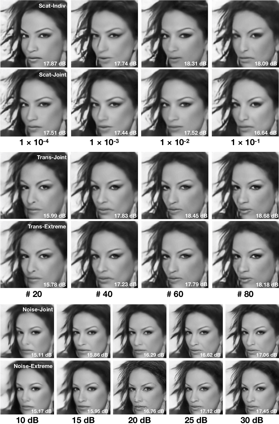
Fig. 2 and Fig. 3 empirically and visually evaluate the robustness of ScaDec regarding to different contrasts $\bm{f}_{\text{\tiny max}}$, numbers of illuminations $\bm{k}$, and input SNR $\bm{s}$. The parametric setting of each test is reported in the corresponding plot. Fig. 2(a) summarizes the performance of ScaDec with respect to different $\bm{f}_{\text{\tiny max}}$. Scat-Indiv estimated the optimal performance by individually training on the data with $\bm{f}_{\text{\tiny max}}$ equals to $1\times 10^{-1}$, $1\times 10^{-2}$, $1\times 10^{-3}$ and $1\times 10^{-4}$, though Scat-Joint was jointly trained on the data corresponding to all levels of $\bm{f}_{\text{\tiny max}}$. The jointly trained ScaDec obtains nearly optimal performance in the sense that the reconstruction SNR of Scat-Joint agrees with that of Scat-Indiv.

Fig. 2(b) and 2(c) illustrate the stability of ScaDec as $\bm{k}$ and $\bm{s}$ vary. The blue lines correspond to the model jointly trained on the data of all the values (marks in the curves), and the orange lines represent the model trained merely on the boundary values (eg. $\bm{k}=10,80$). Both plots clearly show that ScaDec is relatively stable since the degradation of reconstruction SNR is gradual as $\bm{k}$ and $\bm{s}$ shift from the lower limit to the upper limit. For example, the SNR values were 18.29 dB, 19.26 dB, 19.84 dB, and 20.20 dB at $\bm{k}$ equal to 20, 40, 60, and 80, respectively. Moreover, ScaDec shows good ability to generalize since the extreme models matches the joint models at each level of $\bm{k}$ and $\bm{s}$. It is worth of mentioning that data of the in-between levels remained unused by the former models while used by the later ones in the training.

We further explored the performance of ScaDec under extreme conditions. We considered two scenarios: 1) reconstruction from very noisy measurements ($\bm{s}=5$) where common algorithms fail and 2) reconstruction of images with mismatched size ($256\times 256$) whose measurements is nonlinear to the training ones. ScaDec was reported to fail in both scenarios since the measurements are too corrupted to extract useful information and the nonlinear relationship is not easy to generalize. However, ScaDec is stable in the various and further show its potential for applications of diffractive imaging.

References

- [1] Y. Sun, Z. Xia, and U. S. Kamilov, “Efficient and accurate inversion of multiple scattering with deep learning,” Opt. Express, vol. 26, pp. 14678–14688, May 2018.
- [2] J. W. Lim, K. R. Lee, K. H. Jin, S. Shin, S. E. Lee, Y. K. Park, and J. C. Ye, “Comparative study of iterative reconstruction algorithms for missing cone problems in optical diffraction tomography,” Opt. Express, vol. 23, pp. 16933–16948, June 2015.
- [3] D. J. Brady, K. Choi, D. L. Marks, R. Horisaki, and S. Lim, “Compressive holography,” Opt. Express, vol. 17, no. 15, pp. 13040–13049, 2009.
- [4] M. Born and E. Wolf, Principles of Optics, ch. Scattering from inhomogeneous media, pp. 695–734. Cambridge Univ. Press, 7 ed., 2003.
- [5] L. Tian and L. Waller, “3D intensity and phase imaging from light field measurements in an LED array microscope,” Optica, vol. 2, pp. 104–111, 2015.
- [6] U. Kamilov, I. N. Papadopoulos, M. H. Shoreh, A. Goy, C. Vonesch, M. Unser, and D. Psaltis, “A learning approach to optical tomography,” in Frontiers in Optics 2015, p. LW3I.1, Optical Society of America, 2015.
- [7] U. S. Kamilov, I. N. Papadopoulos, M. H. Shoreh, A. Goy, C. Vonesch, M. Unser, and D. Psaltis, “Optical tomographic image reconstruction based on beam propagation and sparse regularization,” IEEE Trans. Comp. Imag., vol. 2, pp. 59–70,, March 2016.
- [8] U. S. Kamilov, D. Liu, H. Mansour, and P. T. Boufounos, “A recursive Born approach to nonlinear inverse scattering,” IEEE Signal Process. Lett., vol. 23, pp. 1052–1056, August 2016.
- [9] E. Soubies, T.-A. Pham, and M. Unser, “Efficient inversion of multiple-scattering model for optical diffraction tomography,” Opt. Express, vol. 25, pp. 21786–21800, September 2017.
- [10] H.-Y. Liu, D. Liu, H. Mansour, P. T. Boufounos, L. Waller, and U. S. Kamilov, “SEAGLE: Sparsity-driven image reconstruction under multiple scattering,” IEEE Trans. Comput. Imaging, vol. 4, pp. 73–86, March 2018.
- [11] T.-A. Pham, E. Soubies, A. Goy, J. Lim, F. Soulez, D. Psaltis, and M. Unser, “Versatile reconstruction framework for diffraction tomography with intensity measurements and multiple scattering,” Opt Express, vol. 26, pp. 2749–2763, February 2018.
- [12] G. Maire, F. Drsek, J. Girard, H. Giovannini, A. Talneau, D. Konan, K. Belkebir, P. C. Chaumet, and A. Sentenac, “Experimental demonstration of quantitative imaging beyond abbe’s limit with optical diffraction tomography,” Phys. Rev. Lett., vol. 102, p. 213905, May 2009.
- [13] S. Arhab, G. Soriano, Y. Ruan, G. Maire, A. Talneau, D. Sentenac, P. C. Chaumet, K. Belkebir, and H. Giovannini, “Nanometric resolution with far-field optical profilometry,” Phys. Rev. Lett., vol. 111, p. 053902, Aug 2013.
- [14] O. Ronneberger, P.Fischer, and T. Brox, “U-net: Convolutional networks for biomedical image segmentation,” in Medical Image Computing and Computer-Assisted Intervention (MICCAI), vol. 9351 of LNCS, pp. 234–241, Springer, 2015. (available on arXiv:1505.04597 [cs.CV]).
- [15] K. H. Jin, M. T. McCann, E. Froustey, and M. Unser, “Deep convolutional neural network for inverse problems in imaging,” IEEE Trans. Image Process., vol. 26, pp. 4509–4522, September 2017.
- [16] J. C. Ye, Y. Han, and E. Cha, “Deep convolutional framelets: A general deep learning framework for inverse problems,” SIAM J. Imaging Sci., vol. 11, no. 2, pp. 991–1048, 2018.
- [17] N. Borhani, E. Kakkava, C. Moser, and D. Psaltis, “Learning to see through multimode fibers,” Optica, vol. 5, pp. 960–966, Aug 2018.
- [18] Z. Liu, P. Luo, X. Wang, and X. Tang, “Deep learning face attributes in the wild,” in Proceedings of International Conference on Computer Vision (ICCV), 2015.