Calculation of the pion-photon transition form factor using dispersion relations and renormalization-group summation
Abstract
We consider the lightcone sum-rule description of the pion-photon transition form factor, based on dispersion relations, in combination with the renormalization group of QCD, in terms of the formal solution of the Efremov-Radyushkin-Brodsky-Lepage evolution equation, and show that the emerging scheme amounts to a certain version of Fractional Analytic Perturbation Theory (FAPT). In order to ensure the correct asymptotic behavior of the considered physical quantity, this modified FAPT version has to be supplemented by process-specific boundary conditions—in contrast to the standard one. However, it provides the advantage of significantly improving the inclusion of radiative corrections in the low-momentum regime of QCD perturbation theory using renormalization-group summation.
pacs
11.10.Hi,12.38Bx,12.38.Cy,12.38.LgI Introduction
The description of hard exclusive hadronic processes in QCD is difficult because it must account for typical nonperturbative phenomena like the hadron binding dynamics and/or long-distance effects pertaining to soft contributions that cannot be assessed by means of perturbative Quantum Chromodynamics (pQCD).
Consider for example the pion-photon transition form factor for two highly virtual photons describing the reaction by assuming that . Applying factorization, the pion-photon transition form factor (TFF) is given by the following correlation function written in a generic convolution form as follows
| (1) | |||||
where and the superscript is the twist label. For simplicity, we have adopted the default scale setting, i.e., , where the abbreviations refer to the factorization and renormalization scales, respectively.
A useful calculational scheme to implement a consistent factorization of short-distance dynamics, amenable to QCD perturbation theory via hard-gluon exchanges, from long-distance phenomena, encoded in nonperturbative hadron distribution amplitudes based on the lightcone operator product expansion (OPE), is provided by lightcone sum rules (LCSR)s [1, 2]. In this scheme, correlation function (1) can be cast in the form of a dispersion relation in terms of the large photon virtuality to obtain a LCSR. This dispersive conceptual picture of exclusive hadronic processes will be a key issue in the present investigation.
The pion-photon TFF represents a prototypical example of such a process and provides valuable information on the quark structure of the pion in terms of its leading twist two (and subleading twist four) distribution amplitudes (DA)s . Moreover, it can be measured in single-tag experiments. A classification of various theoretical predictions in comparison with the available data [3, 4, 5, 6] can be found in [7]. In contrast, the pion DA is not directly measurable but has to be inferred from the data or be constructed from nonperturbative models. In most theoretical analyses, it is reversed engineered from its (first few) moments [8] (see also [9])
| (2) |
where , , , with being the longitudinal momentum fraction carried by the valence quark in the pion. Until now only the second moment has been measured on the lattice, yielding diverging values [10, 11, 12, 13, 14, 15], while there are not enough experimental data to constrain the moments above . For a discussion of these techniques and comparison of various types of pion DAs with the lattice estimates, see [16]. More advanced theoretical aspects of the light-meson DAs have been considered in [17, 18, 19] with arguments based partly on QCD sum rules (SR)s with nonlocal condensates [20, 21, 22, 23]. There are also alternative computational methods, for instance, Dyson-Schwinger equations [24, 25], AdS/QCD [26, 27], etc.
On the other hand, we have in our hands the very powerful method of the QCD renormalization group (RG) that tells us how QCD properties are related to each other at different momentum scales (notably, the strong coupling and dynamical quantities like various parton distribution functions via their anomalous dimensions). A serious problem one encounters when applying QCD perturbation theory is that the running coupling increases logarithmically at low so that the validity of the expansion rapidly deteriorates when , giving rise to the Landau singularity. This affects the proper inclusion of higher-order radiative corrections and the determination of the optimal choice of the renormalization-scale setting procedure considerably [28, 29, 30].
To avoid this problem, analytic versions of the power-series expansion in (better say, non-power expansions) have been proposed by various authors, e.g., [31, 32, 33, 34, 35, 36, 37, 38] (see [39] for a review and further references while more recent developments are discussed, for instance, in [40, 41]). Such schemes make use of dispersion relations in the spacelike and the timelike regions in order to implement causality while preserving the RG properties—see [42] for a broad review of such methods. For our analysis below, we mention explicitly the Analytic Perturbation Theory (APT) [34] and its generalization to any real power of the coupling constant, described by Fractional APT (FAPT) [43].
As already mentioned with respect to the pion-photon TFF, LCSRs enable the calculation of various physical quantities on the basis of dispersion relations. Their main ingredient is a spectral density that can be calculated in terms of the hard-scattering amplitude for the quark-gluon subprocesses order-by-order in QCD perturbation theory. It appears therefore natural to investigate the LCSR approach in conjunction with the renormalization group and see how the LCSR dispersion representation can match a RG-improved perturbative expansion. To achieve this goal, we will have to invent a particular version of FAPT that employs process-dependent boundary conditions on the behavior of the coupling in the deep infrared (IR) regime in order to ensure compliance with the QCD asymptotics. The strategy is to develop a scheme with the advantage of including the RG series of radiative corrections to the TFF at once.
The rest of the paper is organized as follows. In the next section (Sec. II) we expose the key idea of RG improvement by expressing the TFF as a convolution of hard-scattering amplitudes in QCD perturbation theory with the twist-two pion distribution amplitude. Section III deals with the inclusion of radiative corrections into the LCSR using a dispersive representation in conjunction with the RG approach. To realize this goal, we have to “calibrate” the behavior of the FAPT analytic coupling at in such a way as to ensure the correct asymptotic behavior of the TFF at . Drawing on these ideas, we develop an extended version of FAPT—originally developed in [43, 44, 45] with recourse to [46] (see also [28, 29, 30, 47] and [48, 49] for reviews)—by augmenting this perturbation theory with a new analytic charge that amends the conflict between the FAPT analytic couplings at and the asymptotic behavior of the TFF following from QCD. In Sec. IV we discuss how the soft, i.e., quasi-real photon in the TFF, relevant for single-tag experiments, can be accommodated within the new FAPT framework. Phenomenological implications of our theoretical scheme are discussed in Sec. V. Our conclusions are given in Sec. VI, while some important technical issues are treated in three Appendices.
II TFF with RG improvement
In this section we consider the pion-photon TFF in convolution form [50, 51, 52] and perform a RG summation with the aim to obtain a LCSR in terms of an improved dispersion relation (see Sec. III). The key idea of our procedure here and below is the following. We combine causality, encoded in the dispersion relations of LCSRs, with RG invariance, which induces analyticity of the perturbative expansion in order to transfer the power-series expansion of the pion-photon TFF in terms of the usual QCD coupling (and its powers), exhibiting ghost singularities, into a functional expansion over singularity-free “calibrated” analytic couplings that preserve the UV asymptotics of this observable. Let us now enter the formal description of this task.
At the twist-two (tw) level, the amplitude for the hard process , where the two photon virtualities are subject to the condition and , can be written in the general form (referring for the partial cases of the TFF to [53, 51])
| (3) | |||||
where we have incorporated the general solution of the RG equation for the QCD charge pertaining to the -function, , by . Moreover, we have introduced the coupling parameter with and the color factor , whereas the pion decay constant has the value MeV. The other elements of the above equation have the following meaning: is the Born term of the hard-scattering amplitude, , and is the coefficient function of the quark-gluon subprocess at the loop order , where denotes the evolution kernel related to the perturbative expansion of the Efremov-Radyushkin-Brodsky-Lepage (ERBL) evolution equation [54, 55]. For convenience later on, we have also introduced the abbreviation that represents the effective virtuality of the “hand-bag” diagrams.
The integration over in (3) is possible for large enough values of , at least for , so that one remains within the allowed range of pQCD. Strictly speaking, one has to employ in order to ensure that the calculations are performed within the domain of applicability of the factorization approach of pQCD. At the one-loop level, the next-to-leading-order (NLO) coefficient function is and Eq. (3) reduces in the basis of the Gegenbauer harmonics to
| (4a) | |||||
| (4b) | |||||
The above equation follows from the relations
| (5) |
where denotes the one-loop anomalous dimension of the corresponding composite operator of leading twist with . Finally, the function represents the th-harmonic contribution in the conformal expansion of , i.e.,
| (6) |
Because the moments () and the conformal coefficients are interrelated, once the moments of the DA have been extracted, one can compute a subset of within a margin of theoretical uncertainties at the same normalization scale [56]. Employing expansion (6), the leading twist TFF in Eq. (3) reads
| (7) |
By virtue of , practically reduces to the set of , while the ERBL evolution in (4) is governed by the powers .
Thus, the reduced formula (4b) accumulates the one-loop RG running of and also the analogous one entering the common ERBL factor to all orders of the perturbative expansion. The contribution of the zeroth-order harmonic assumes the simplest form , due to the current conservation . Therefore, in this case, expression (4b) finally reduces to
| (8) |
Expanding and the ERBL factors in (4b), one recovers the results stemming from the radiative corrections to the TFF at the next-to-next-to-leading order (NNLO) level [52]. Indeed, within the framework of fixed-order perturbation theory (FOPT), the hard-scattering amplitudes have the following structure
| (9) |
The various radiative corrections are given by
| (10a) | |||||
| (10b) | |||||
| (10c) | |||||
where . The underlined terms in Eq. (10) pertain to the running coupling and the common ERBL factor in Eq. (4). The remaining plain terms represent the one-loop, , and the two-loop, , corrections, respectively—cf. Eq. (3), first line. Finally, the double underlined term in Eq. (10c) marks the beginning of the next “tower” of two-loop corrections to the common term and the ERBL factor in the general expression given by Eq. (3). The explicit expressions for and are presented in Appendix A, while the equations for and the elements of and related references can be found in Appendix A in [52].
Let us emphasize at this point that one cannot directly use the formulas given by (4) for small — even if is large. The reason is that for , these expressions run out of their applicability domain allowed by the “factorization conditions” mentioned before in this section. Indeed, the scale argument becomes for smaller than and hence unprotected. For this reason, we do not use the complete result of the RG summation at small , but employ instead the FOPT one, see, for instance, Sec. 2 in Ref. [52]. The situation changes completely when one applies the results expressed via Eqs. (4), (10) to a dispersion relation as we are now going to show.
III Radiative corrections to the TFF using a dispersive representation
The aim in this section is to discuss the radiative corrections to the pion-photon TFF using the dispersion-relation representation that forms the basis of the sum rules on the lightcone [2] (see also [57] for a more recent exposition of the method).
In this formalism, the TFF satisfies the following dispersion relation
| (11) |
where , as before, while the spectral density reads
| (12) |
In the Born approximation, 1l is the only term that contributes to Eq. (4b). It provides the well-known result [2]
| (13) |
where sets the scale for the twist-four contribution and is an effective pion DA of twist four. The above expression is induced by the particular discontinuity of the imaginary part of the Born amplitude , i.e.,
| (14) |
In the framework of FOPT it is clear that higher-order corrections to also contribute owing to the logarithmic factors in the Born amplitude [51, 58]. Our goal below will be to obtain the radiative corrections within the LCSR formalism on the ground of the results in Eqs. (4) and (8) obtained by RG summation. As we will see in the next subsection, this procedure will inevitably lead to an analytic version of QCD perturbation theory which amends by construction Landau-type singularities.
III.1 Key element of the radiative corrections in the dispersive representation
The RG summation of all radiative corrections to the TFF in Eq. (4) provides another possibility to extract the imaginary part of the TFF and get the spectral density [2, 51, 52]. Indeed, for the Born contribution, the corresponding imaginary part is generated by the singularity of (multiplied by powers of logarithmic terms, see Eq. (13) and the text below it), while the imaginary part after the RG summation of the radiative corrections originates also from the contributions.
The general expression for the key perturbative element in this procedure follows from the first term in Eq. (4b) and amounts to the following integral, termed :
| (15a) | |||||
| (15b) | |||||
| The contribution to the partial TFF can be expressed in the form of a convolution between the term , contained in , and the remainder of the partial harmonic . The latter includes either the next radiative correction , or the Born term —see Eq. (4b). After changing the integration variable , and applying the principal-value prescription | |||||
| we set to obtain for the integral in Eq. (15b) the expression | |||||
| (15c) | |||||
The second term in Eq. (15c) containing the function is induced by the singularity of in Eq. (15b). But, in contrast to the Born case in Eq. (14), this contribution vanishes for the running coupling . This can be explicitly seen in the case of the one- and two-loop running. Therefore, only the first term in Eq. (15c) survives, where defines the FAPT spectral density , i.e.,
| (16) |
Thus, the key element can be expressed in terms of the corresponding FAPT couplings. For the perturbative spectral density , we employ the standard FAPT expression [43]
| (17) |
where the phase and the radial part have an -loop content (see [44] and Appendix B), whereas .
Having in mind further considerations to be exposed later, we define here a more general class of spectral densities by inventing a possible gap in the variable , expressed via the scale , . Inserting into Eq. (16), we obtain for the dispersion integral at the lower limit , notably,
| (18) |
Now the RHS of in Eq. (18) can be decomposed in terms of a new coupling and the standard FAPT couplings and , known from [43, 44]:
| (19a) | |||
| (19b) | |||
| (19c) | |||
Note that the structure of a subtraction in the square brackets in Eq. (18) follows from the decomposition of the integrand in the RHS of (19a). Some remarks regarding Eq. (19) are here in order. First, the FAPT couplings [43] and [44] refer to the spacelike and the timelike regime, respectively. Second, the integral represents a generalization of the previous two FAPT couplings, as it becomes obvious from Eq. (19c) and from the detailed exposition in Appendix B.
We close this discussion by formally defining a new effective coupling , already encountered in (18), that will be used in the next sections, viz.,
| (20a) | |||
| The derivation of in terms of the new FAPT coupling represents a novelty of the present approach. At the same time bears through it a process dependence stemming from the Born term. This dependence enters via the arguments , like in the original case of , but also through the argument at the lower limit of the dispersion integral. Note that for , one has | |||
| (20b) | |||
due to Eq. (19c).
III.2 Pion-photon TFF within FAPT
Before we continue let us i) summarize our findings for the dispersion integral , ii) construct a particular version of the TFF, and iii) consider it at different scales.
i) The general expression for , that includes all involved scales, reads
| (21a) | |||||
| (21b) | |||||
It is instructive to compare the above results with the initial expressions given by Eqs. (4b) and (8). One observes that Eqs. (21a) and (21b) have the same structure as the original expressions and can be recast into the form of Eq. (4b) and Eq. (8), respectively, using the evident replacement .
ii) We show next the results for in the limits , and in explicit form:
| (22a) | |||||
| (22b) | |||||
These equations can again be related to the initial expressions given by Eqs. (4b) and (8) by means of the replacement .
iii) Definition (20a) of the effective coupling , supplemented by Eqs. (21) and (22), reveals that the high-energy asymptotic behavior of the form-factor components is determined in part by the low-energy behavior of or the value of for . Thus, determining the low-energy behavior of the FAPT couplings, one would be in the position to extract information about the high-energy behavior of the transition form factor—an arguably unexpected result that demands a rigorous explanation.
III.3 Low-energy modification of FAPT—calibration procedure
However, this seemingly obvious connection doesn’t work because it causes a spurious contribution to the asymptotic value of the TFF that contradicts pQCD. Indeed, for the effective couplings of analytic perturbation theory (APT) one has according to (B.2) , which entails a sign flip of the radiative corrections due to the second term . Moreover, for , [34, 32, 33] and . If one would substitute these expressions into Eq. (22a), one would immediately arrive at a result for the asymptotic (scaled) TFF that would clearly contradict the limit derived with pQCD in the asymptotic regime. This contradiction in the behavior of can be traced back to the radiative corrections to the inverse moment that are created just by the disturbing term . In fact, the deviation from the standard contribution, proportional to , can be estimated from Eq. (22a), see [51], to be given by the following distortion term
| (23) |
The quantity is a large constant, comparable to the Born term (with ), that certainly destroys the asymptotic behavior of . The latter turns out to be larger than the asymptotic limit already in the vicinity of the normalization scale GeV, as one can see from the behavior of the solid line in the right panel of Fig. 1, and disagrees with the analogous result obtained in the left panel within pQCD. Such a situation calls for a remedy.
To restore the correspondence of our perturbative expansion to the standard pQCD theory, we have to eliminate the distortion term to the TFF at by appropriately adjusting the mathematical IR behavior of the new analytic couplings in such a way as to preserve the validity of the QCD asymptotics applicable to this particular physical process. This can be achieved by imposing the condition in , which is tantamount to a “calibration” of their behavior in Eq. (20a).
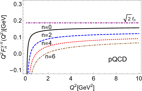
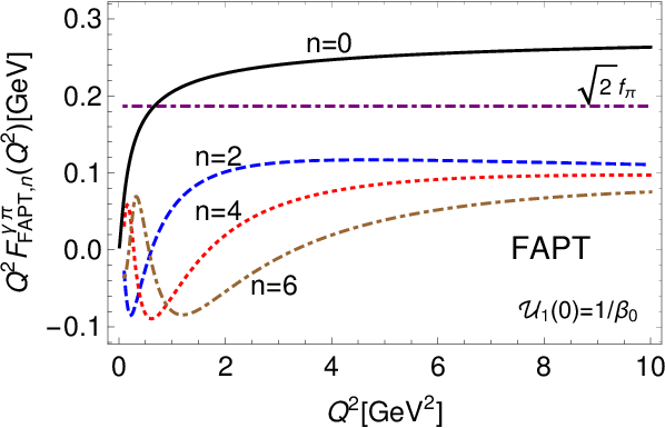
The calibration procedure has more consequences. Consider noninteger values of the index within FAPT. Then the unbounded behavior of the FAPT couplings at one loop for , near would render the corresponding expressions in Eqs. (21b), (22b) meaningless (with the related details being given in Appendix B). Consequently, in order to obtain a TFF with the correct behavior in the asymptotic regime, we have to set
| (24) |
also for for . This implies that the initial FAPT couplings, which were constructed without employing any nonperturbative input at low momenta to saturate them in the deep IR regime, should be corrected at a posteriori in order to avoid spurious, i.e., unphysical constants. Thus, the present scheme represents an advance over the original FAPT and corrects the corresponding expressions for the analytic couplings displayed in the middle columns of Eqs. (50) in Appendix B. Note that the imposition of calibration is a novelty of the present investigation and differs from other approaches that try to model the low-energy behavior of the couplings [59, 60, 61]. The difference relative to [59] arises from the imposition at small fixed value , while in [60, 61] one sets (when ) as suggested by lattice simulations [62] for dressing functions. In any case, the above redefinition based on calibration renders the TFF compatible with the QCD asymptotic limit for , as one can see from the last column in Eq. (50). In what follows, we will refer to this calibrated version of FAPT as “cal-FAPT”. As one sees from the right panel of Fig. 2, this version of FAPT guarantees that the TFF behavior subject to condition (24) indeed reproduces the pQCD limit and the TFF result for — left panel — in contrast to the behavior entailed by the standard FAPT couplings, see Fig. 1 (solid line for in the right panel). In contrast, the calibrated counterpart of the TFF shows excellent agreement with the PQCD result as it is effected in the right panel of Fig. 2.


IV Hadronic photon content in LCSR
In the previous section we have constructed a new perturbative expansion that includes all radiative corrections to the TFF using RG summation while preserving its QCD asymptotics. In this section, we are going to implement this scheme to the LCSR formulation in terms of the calibrated FAPT.
To this end, let us extend the initial expression for the pion TFF in the LCSR, given by Eq. (11), to the case of a quasi-real photon with a virtuality . This can be done in terms of a physical spectral density that takes into account the vector-meson properties of the quasi-real photon. Employing the physical spectral density with we substitute into (11), to obtain [2]
| (25) |
where the term in the physical spectral density models the -resonances. Applying the “duality approximation”, that involves the TFF to describe the intermediate subprocess (see Sec. 2 in [2] for details), we find
| (26a) | |||
| From the Borel transform of (26a), we get | |||
| (26b) | |||
finally arriving at the total TFF expression for [2], evaluated in the limit , i.e.,
| (27) |
where is the Borel parameter. We use for simplicity, the fixed value GeV2. Increasing the Borel mass to GeV2 would affect the TFF between 10 and 40 GeV2 only by about [63], which shows that its influence on the TFF is small, see also [57]. For a more sophisticated treatment, we refer to our previous works, e.g., [16].
The first term in Eqs. (25) and analogously in (27) stems from the hard (i.e., quark-gluon) part with the integration taken over the duality interval . Here plays the role of the main scale parameter in the model of the physical density. Note that for , expression (27) reduces to the first term, i.e., to the initial form of Eq. (11), and further to the harmonic expansions encountered in Eqs. (21) and (22). The numerical value of the effective threshold parameter in the -meson channel is fixed to the value GeV2, see, for instance, [50]. The second term in Eq. (27) is the result obtained for the TFF following from Eq. (26b) and originates from the soft (i.e., hadronic) part of the pion TFF. For the considerations to follow, it is useful to reduce Eq. (27) to the Born approximation by taking for the expression in (13) and by replacing the variable of integration to get
| (28b) | |||||
| where . The twist-four term depends on the parameter , which assumes values in the interval GeV2 [64]. Below we shall use the elements of the expansion expressed in terms of the Gegenbauer harmonics, i.e., , where | |||||
| (28c) | |||||
Note that in this expression we combined the twist-four contribution with the component of the twist-two spectral density into a single spectral density termed .
IV.1 Hard part of LCSR with RG summation
The first term in Eq. (27), notably,
| (29) |
represents the hard (label H) contribution to the LCSR and can be directly expressed in terms of FAPT. The only difference with respect to Eqs. (21), (22), is the lower limit of integration instead of zero. This shift induces a more complicated structure of the effective coupling as it now depends on two scale-parameters: and . Performing similar calculations as those to derive Eq. (18) for the key element in Subsection III.1, we derive the following expression
| (30a) | |||||
| (30b) | |||||
| where we have imposed the condition (see for the general expression given by Eq. (C) Appendix C). The effective coupling is a continuous function in the vicinity of and , as it follows from the definitions in Eq. (30b). Note that in the limit , in Eq. (30a) becomes | |||||
| (30c) | |||||
where and . Let us conclude these considerations by presenting the harmonic representation for the hard part in Eq. (29):
| (31a) | |||||
| (31b) | |||||
The first entry in Eq. (31a) pertains to the contribution of the zero-harmonic in the expansion of the first term in Eq. (28b). The structure of the next entry in Eq. (31a)—which represents the radiative correction related to —is more interesting because the first term in Eq. (30c) (simplified by setting ) corresponds to the integration over the expected hard region , while in the region a new contribution from the second term appears in addition. On the other hand, the limit , (or 0) in the hard part of Eqs. (31a), (31b) reproduces the known FAPT result encountered in Eqs. (22a), (22b).
IV.2 Soft part of LCSR with RG summation
We consider now the soft part of the LCSR expressed by (27). The quasi-real photon induces a contribution that is encoded in and can be expressed within FAPT as follows
| (32) |
The term was already discussed in connection with Eq. (21). Taking it into account and employing the definition of the effective coupling, we obtain
| (33a) | |||||
| (33b) | |||||
| (33c) | |||||
where the first term in Eq. (33a) corresponds to the zero-harmonics part of the second term in Eq. (28b). Note that a new coupling appears in these equations, which originates from the differences written in the form
| (34a) | |||||
| (34b) | |||||
One can see from Eqs. (33) and (34) that the integration domain for the radiative corrections is the same as for the Born term in (33a). Moreover, the standard structure of the integral is restored, while the quantity plays the role of an effective coupling in the soft part.
Expressions (33b), (33c) are derived by assuming that the effective coupling does not depend (by means of the function ) on and is taken at , i.e., . This approximation is justified, provided depends on in a significantly weaker way than . We shall consider the conditions for the validity of this approximation farther below.
Let us now concentrate our attention on the complete LCSR result for the TFF by combining the soft part (denoted by S) in (33)
| (35) |
with the hard part given by Eqs. (29) and (31). Substituting Eqs. (29) and (35) into the initial Eq. (25), we arrive at the final equation for :
| (36) |
This equation is the FAPT analogue of the LCSR given by Eq. (27). However, it possesses some advantages relative to that and includes some new effects: (i) It has no singularities in the perturbative expansion (cf. Eq. (4)). (ii) It contains all logarithmic power corrections by virtue of the RG-summation (taken here in the one-loop approximation), while the values of these corrections are smaller in comparison to those in standard pQCD using FOPT—thus significantly improving the reliability of the perturbative expansion. (iii) It takes into account the particular low-energy behavior of the quasi-real photon within the LCSR approach.
V Effect of RG summation on the TFF in LCSR
From the calculational point of view, this FAPT-inspired approach may help avoid the appearance of large radiative corrections to the pion-photon TFF at low/moderate momenta because such terms become small by virtue of the FAPT summation in contrast to FOPT. Indeed, the smallness of the next-order FAPT coupling in Fig. 4, shown in App. B by a shaded area at the bottom of the 3D graphics explicitly illustrates this feature.
The content of the RHS of the general LCSR expression (36) for the pion-photon TFF can be recast in terms of the –expansion, cf. Eq. (7), to obtain
| (37) |
where the expressions for the partial TFFs follow from Eqs. (31) and (33). To simplify the final representation of , as well as for further analysis in future work, we use the effective couplings for from Eq. (30c) and Eq. (34b) so that we arrive at
| (38a) | |||||
| (38b) | |||||
| (38c) | |||||
| (38d) | |||||
where the functions and are defined analogously to (34a) and (34b), and denote the effective couplings entering the soft part. The two equations above represent our final expressions for the TFF in the dispersive form of RG augmented LCSRs and encapsulate the calibrated FAPT expansion for this quantity. Let us also supply some important remarks. First, the Born contribution in Eq. (38a) coincides with the standard one for the zero-harmonic, see Eq. (28) (where ), while all further corrections in (38b), (38c), and (38d) appear as the result of the FAPT summation of the radiative corrections (see Sec. IV). Second, their contributions bear the same minus sign and for momentum transfers in the range GeV2 have a magnitude a few times smaller than the FOPT results [51, 57]. The important element of these corrections, i.e., the convolution term , is given in App. A. Third, by significantly reducing the size of the radiation corrections, the actual constraint for the applicability of the LCSR approach resides with the high-twist contributions that become important for .

In order to test the capabilities of the new scheme in more real terms, we illustrate in Fig. 3 its application to the TFF in comparison with the experimental data. This version of the figure implements the corrections done in the included Erratum. For the sake of definiteness, we employ the family of the bimodal BMS pion DAs, obtained in [65]. The corresponding results for the TFF are shown in the form of a green strip which quantifies the variation of these DAs in terms of their coefficients with the Gegenbauer decomposition in Eq. (6) (for derivation and justification see [65, 18, 52] and references therein).
The predictions shown in Fig. 3 are obtained by employing the values of these coefficients at the normalization scale [50, 56] that are given by 11 1 The values and are strongly correlated along the line const.. The other LCSR parameters have been fixed by previous investigations to the values [2, 64] , GeV2, GeV2, GeV , and and are not varied here.
Using Eq. (37) and the partial TFF terms from Eqs. (38), we obtain for the prediction shown by the solid black line in Fig. 3. The (green) strip enveloping this curve indicates the admitted theoretical variations of the BMS DA in terms of and , while other uncertainties are not considered here. The interested reader can find estimates of the various theoretical uncertainties entering the TFF calculation in [52, 63]. It is worth noting that the platykurtic pion DA [17] yields very similar TFF predictions to the BMS-like DAs and has, therefore, been omitted in Fig. 3—[66].
The presented prediction is in good agreement with all experimental data, especially in the low/moderate region of GeV2, as comparison with the LCSR result in Fig. 4 of [66] also reveals, though a more detailed comparison requires additional analysis. The achieved agreement with the experimental data results from the decrease of the negative contribution of the resummed radiative corrections within the applied dispersion representation together with the twist-six contribution, see the included Erratum. We restrict ourselves in this work to this qualitative observation, while a full-fledged analysis of the experimental data within the presented elaborated FAPT-LCSR approach will be carried out in future work. For phenomenological purposes such analysis appears particularly useful for the expected low-momentum data of the BESIII Collaboration.
VI Conclusions
In this work we considered the TFF and proposed an approach, which combines the method of LCSRs based on dispersion relations, with the renormalization group summation expressed in terms of the formal solution of the ERBL evolution equation. We argued that this procedure gives rise to a particular version of FAPT [43, 44] and worked out the technical details.
The advantage of the obtained calibrated FAPT scheme pertains to process-dependent boundary conditions imposed on the analytic versions of the couplings in the deep infrared region in order to preserve the asymptotic behavior of the TFF prescribed by perturbative QCD. The resulting theoretical scheme provides the possibility to include the infinite series of radiative corrections to the considered TFF via RG summation. The involved techniques are exposed in the text with more calculational details being given in three dedicated appendices.
Though our focus in this work was primarily on the methodological aspects of the new framework, we also provided a qualitative phenomenological application to show the effect on the TFF of the RG summation of the radiative corrections. To this end, we presented a qualitative prediction for the scaled TFF employing BMS-like pion DAs, which we show in Fig. 3 for low to intermediate values in comparison with the existing data. This version of the figure complies with the included Erratum. We argue that the use of the RG-improved LCSR provides an improvement relative to the standard LCSR method based on FOPT—especially at low [52]. Dedicated analysis of the asymptotic regime of the TFF in theory and in terms of the experimental data will be given in [67].
Acknowledgements.
We would like to thank A. V. Pimikov for useful discussions. This work was partially supported by the Heisenberg-Landau Program (Grants 2017 and 2018), the JINR-BelRFFR grant F16D-004, by the FONDECYT Postdoctoral Grant No. 3170116, and by FONDECYT Regular Grant No. 1180344.Appendix A Next-order perturbation elements
The coefficient function of the partonic subprocess and the evolution kernel ,
| (39) | |||||
| (40) |
are determined by the elements
| (41a) | |||||
| (41b) | |||||
where the symbol means
.
The expression for the key convolution term
in the harmonic expansion can be significantly simplified to get
| (42) | |||||
| (43) | |||||
| (44) |
see Appendix A in [51]. The quantities and are the eigenvalues of the elements and of the one-loop kernel in Eq. (40), respectively. Expression denotes the elements of a calculable triangular matrix (omitted here) — see for details [51, 57].
Appendix B Analytic properties of FAPT couplings
B.1 Initial FAPT couplings
In this Appendix we give the expressions for the standard one-loop running couplings and their FAPT counterparts. To facilitate the representation, we express them in terms of the auxiliary variable , multiplied for simplicity by the term . In other words, we shift the origin of the different coupling images to the values ,
| (45a) | |||||
| (45b) | |||||
| (45c) | |||||
| where the symbol is used to denote the function argument, clearly distinguishing it from the dependence.22 2 An expression analogous to (45c) was derived long ago in [68, 69] in connection with multiloop calculations and the Higgs-boson decay into hadrons. The spectral density has the form () | |||||
| (45d) | |||||
Here, is the “pole remover”, expressed in terms of the Lerch transcendental function [43]. The following equation
| (46) |
determines the analytic continuation into the outer region of the radius of convergence, making use of the Hurwitz zeta function . The first few terms of its asymptotic expansion for are given by [70]
| (47) |
Using this asymptotic expansion for (which corresponds to ) and for , we obtain for Eq. (46) the following expression
| (48) |
By substituting the asymptotic form of this equation into (45b), we get
| (49) |
where the second term leads to a divergence in the limit when . Employing Eqs. (49) and (45c), one can then obtain the range of values of the functions , notably,
| (50a) | |||||
| (50b) | |||||
One observes that the couplings become unbounded in the vicinity of and . In some sense, the well-known singularity of the standard running coupling in Eq. (45a) for and turns in the limit into a singularity of the FAPT couplings for , cf. (45b) and (45c). Therefore, these results for cannot be directly used in the vicinity of and , where the FAPT couplings are ill-defined. One needs to “calibrate” these couplings in this regime by demanding that they vanish. This intervention guarantees at the same time that observables calculated with them, e.g., the TFF, have the correct UV asymptotics following from pQCD. To this end, we redefine the couplings in the vicinity of and for , to be , while the behavior of these couplings for remains unaffected.
B.2 Generalized FAPT coupling
During the calculation considered in Subsec. III.1, a new, more general, two-argument coupling appeared “naturally” in Eq. (19), viz.,
| (54) |
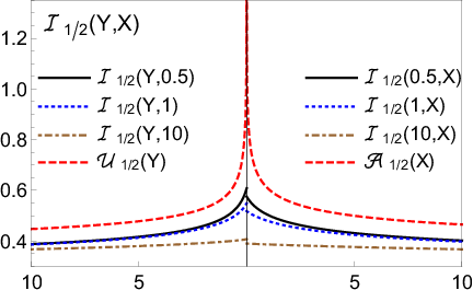
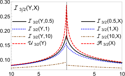
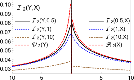
The coupling is regular for , while for or it reduces to the initial FAPT couplings in accordance with Eq. (54). The behavior of with respect to the arguments is illustrated in Fig. 4, while the graphics showing its behavior when one of its arguments is fixed is displayed in Fig. 5. These figures are corrected versions of the published ones after removing an error in the code—see the Erratum below. One appreciates in this figure the smallness of the next-order FAPT coupling .


Appendix C Two scales effective coupling
Here we outline the calculation of the key element of the dispersion integral discussed in Sec. IV.1, viz.,
| (55) |
at the low limit . After changing the integration variable to , the low limit becomes . The value of the low limit of this function leads to a new constraint for the range of integration in the variable , notably, . On the other hand, if , one should start to integrate with , where . In the range , one then obtains
| (56) |
while for the case only the second term survives, i.e.,
| (57) |
Substituting Eq. (18) into Eq. (56), one arrives at the final expression for ,
| (58) | |||||
where and the couplings and appear as the limits of by allowing their arguments to approach zero, cf. (19c). The effective coupling , following from Eqs. (56), (57), reads
whereas the quantity in the vicinity of for is a continuous function as it follows from the properties expressed in (19c). In the limit , one has , which completes the argument.
ERRATUM
The graphics shown in the right panels of Figs. 1 and 2 of the journal version are the result of an erroneous computer code. The corresponding corrected curves are displayed here in Fig. 6.


Analogously, also the predictions shown in Fig. 3 in the journal are wrong. The correct contribution to the TFF, comprising the twist-two and twist-four terms, is shown as a dashed line in Fig. 7 below.
As one sees, FAPT resummation of the radiative corrections induces a sizeable suppression of the transition form factor. To get agreement with the experimental data, it is mandatory to include into expression (36) the twist-six contribution. This is done by taking into account the spectral density for the initial LCSR in Eq. (28), the corresponding contribution [57, 52], given by
| (63) |
where and GeV6 [57]. The resulting TFF is shown in the figure in terms of a solid line. Thus, the conclusion drawn in the journal version that one gets agreement with the data by taking into account only the twist-two and twist-four terms has to be corrected accordingly.

The deviations of the results given in Figs. 4 and 5 of the journal version differ from their corrected counterparts by less than about 5 percent and are therefore not shown here.
Acknowledgements.
We would like to thank Alex Pimikov for help with the numerical computations.References
- [1] I. I. Balitsky, V. M. Braun, and A. V. Kolesnichenko, Nucl. Phys. B312, 509 (1989).
- [2] A. Khodjamirian, Eur. Phys. J. C6, 477 (1999), eprint hep-ph/9712451.
- [3] H. J. Behrend et al. (CELLO), Z. Phys. C49, 401 (1991).
- [4] J. Gronberg et al. (CLEO), Phys. Rev. D57, 33 (1998), eprint hep-ex/9707031.
- [5] B. Aubert et al. (BaBar), Phys. Rev. D80, 052002 (2009), eprint 0905.4778.
- [6] S. Uehara et al. (Belle), Phys. Rev. D86, 092007 (2012), eprint 1205.3249.
- [7] A. P. Bakulev, S. V. Mikhailov, A. V. Pimikov, and N. G. Stefanis, Phys. Rev. D86, 031501(R) (2012), eprint 1205.3770.
- [8] V. L. Chernyak and A. R. Zhitnitsky, Phys. Rept. 112, 173 (1984).
- [9] N. G. Stefanis, Eur. Phys. J. direct C7, 1 (1999), eprint hep-ph/9911375.
- [10] V. M. Braun et al., Phys. Rev. D74, 074501 (2006), eprint hep-lat/0606012.
- [11] V. M. Braun, S. Collins, M. Göckeler, P. Pérez-Rubio, A. Schäfer, R. W. Schiel, and A. Sternbeck, Phys. Rev. D92, 014504 (2015), eprint 1503.03656.
- [12] R. Arthur, P. A. Boyle, D. Brömmel, M. A. Donnellan, J. M. Flynn, A. Jüttner, T. D. Rae, and C. T. C. Sachrajda, Phys. Rev. D83, 074505 (2011), eprint 1011.5906.
- [13] J. Segovia, L. Chang, I. C. Cloët, C. D. Roberts, S. M. Schmidt, and H.-s. Zong, Phys. Lett. B731, 13 (2014), eprint 1311.1390.
- [14] G. S. Bali, V. M. Braun, M. Göckeler, M. Gruber, F. Hutzler, P. Korcyl, B. Lang, and A. Schäfer (RQCD) (2017), eprint 1705.10236.
- [15] G. S. Bali, V. M. Braun, B. Gläßle, M. Göckeler, M. Gruber, F. Hutzler, P. Korcyl, A. Schäfer, P. Wein, and J.-H. Zhang (2018), eprint 1807.06671.
- [16] A. P. Bakulev, S. V. Mikhailov, A. V. Pimikov, and N. G. Stefanis, Phys. Rev. D84, 034014 (2011), eprint 1105.2753.
- [17] N. G. Stefanis, Phys. Lett. B738, 483 (2014), eprint 1405.0959.
- [18] N. G. Stefanis, S. V. Mikhailov, and A. V. Pimikov, Few Body Syst. 56, 295 (2015), eprint 1411.0528.
- [19] N. G. Stefanis and A. V. Pimikov, Nucl. Phys. A945, 248 (2016), eprint 1506.01302.
- [20] S. V. Mikhailov and A. V. Radyushkin, JETP Lett. 43, 712 (1986), [Pisma Zh. Eksp. Teor. Fiz. 43, 551 (1986)].
- [21] S. V. Mikhailov and A. V. Radyushkin, Sov. J. Nucl. Phys. 49, 494 (1989), [Yad. Fiz. 49, 794 (1988)].
- [22] S. V. Mikhailov and A. V. Radyushkin, Sov. J. Nucl. Phys. 52, 697 (1990), [Yad. Fiz. 52, 1095 (1990)].
- [23] S. V. Mikhailov and A. V. Radyushkin, Phys. Rev. D45, 1754 (1992).
- [24] L. Chang, I. C. Cloet, J. J. Cobos-Martinez, C. D. Roberts, S. M. Schmidt, and P. C. Tandy, Phys. Rev. Lett. 110, 132001 (2013), eprint 1301.0324.
- [25] K. Raya, L. Chang, A. Bashir, J. J. Cobos-Martinez, L. X. Gutiérrez-Guerrero, C. D. Roberts, and P. C. Tandy, Phys. Rev. D93, 074017 (2016), eprint 1510.02799.
- [26] S. J. Brodsky, F.-G. Cao, and G. F. de Téramond, Phys. Rev. D84, 033001 (2011a), eprint 1104.3364.
- [27] S. J. Brodsky, F.-G. Cao, and G. F. de Téramond, Phys. Rev. D84, 075012 (2011b), eprint 1105.3999.
- [28] N. G. Stefanis, W. Schroers, and H.-C. Kim, Phys. Lett. B449, 299 (1999), eprint hep-ph/9807298.
- [29] N. G. Stefanis, W. Schroers, and H.-C. Kim, Eur. Phys. J. C18, 137 (2000), eprint hep-ph/0005218.
- [30] A. P. Bakulev, K. Passek-Kumerički, W. Schroers, and N. G. Stefanis, Phys. Rev. D70, 033014 (2004a), eprint hep-ph/0405062.
- [31] G. Grunberg, Phys. Rev. D29, 2315 (1984).
- [32] K. A. Milton and I. L. Solovtsov, Phys. Rev. D55, 5295 (1997), eprint hep-ph/9611438.
- [33] K. A. Milton and O. P. Solovtsova, Phys. Rev. D57, 5402 (1998), eprint hep-ph/9710316.
- [34] D. V. Shirkov and I. L. Solovtsov, Phys. Rev. Lett. 79, 1209 (1997), eprint hep-ph/9704333.
- [35] G. Grunberg (1997), eprint hep-ph/9705290.
- [36] A. V. Nesterenko, Phys. Rev. D62, 094028 (2000), eprint hep-ph/9912351.
- [37] A. V. Nesterenko, Int. J. Mod. Phys. A18, 5475 (2003), eprint hep-ph/0308288.
- [38] B. A. Magradze, Int. J. Mod. Phys. A15, 2715 (2000), eprint hep-ph/9911456.
- [39] D. V. Shirkov and I. L. Solovtsov, Theor. Math. Phys. 150, 132 (2007), eprint hep-ph/0611229.
- [40] G. Cvetic and A. V. Kotikov, J. Phys. G39, 065005 (2012), eprint 1106.4275.
- [41] A. V. Nesterenko, Eur. Phys. J. C77, 844 (2017), eprint 1707.00668.
- [42] A. V. Nesterenko, Strong interactions in spacelike and timelike domains: dispersive approach (Elsevier, 2016), ISBN 9780128034484, URL https://www.elsevier.com/books/strong-interactions-in-spaceli%ke-and-timelike-domains/nesterenko/978-0-12-803439-2.
- [43] A. P. Bakulev, S. V. Mikhailov, and N. G. Stefanis, Phys. Rev. D72, 074014 (2005a), [Erratum: Phys. Rev. D72, 119908 (2005)], eprint hep-ph/0506311.
- [44] A. P. Bakulev, S. V. Mikhailov, and N. G. Stefanis, Phys. Rev. D75, 056005 (2007), [Erratum: Phys. Rev. D77, 079901 (2008)], eprint hep-ph/0607040.
- [45] A. P. Bakulev, S. V. Mikhailov, and N. G. Stefanis, JHEP 06, 085 (2010), eprint 1004.4125.
- [46] A. I. Karanikas and N. G. Stefanis, Phys. Lett. B504, 225 (2001), [Erratum: Phys. Lett. B636, no.6, 330 (2006)], eprint hep-ph/0101031.
- [47] A. P. Bakulev, A. I. Karanikas, and N. G. Stefanis, Phys. Rev. D72, 074015 (2005b), eprint hep-ph/0504275.
- [48] A. P. Bakulev, Phys. Part. Nucl. 40, 715 (2009), eprint 0805.0829.
- [49] N. G. Stefanis, Phys. Part. Nucl. 44, 494 (2013), eprint 0902.4805.
- [50] A. P. Bakulev, S. V. Mikhailov, and N. G. Stefanis, Phys. Rev. D67, 074012 (2003), eprint hep-ph/0212250.
- [51] S. V. Mikhailov and N. G. Stefanis, Nucl. Phys. B821, 291 (2009), eprint 0905.4004.
- [52] S. V. Mikhailov, A. V. Pimikov, and N. G. Stefanis, Phys. Rev. D93, 114018 (2016), eprint 1604.06391.
- [53] B. Melić, D. Müller, and K. Passek-Kumerički, Phys. Rev. D68, 014013 (2003), eprint hep-ph/0212346.
- [54] A. V. Efremov and A. V. Radyushkin, Theor. Math. Phys. 42, 97 (1980).
- [55] G. P. Lepage and S. J. Brodsky, Phys. Rev. D22, 2157 (1980).
- [56] A. P. Bakulev, S. V. Mikhailov, and N. G. Stefanis, Annalen Phys. 13, 629 (2004b), eprint hep-ph/0410138.
- [57] S. S. Agaev, V. M. Braun, N. Offen, and F. A. Porkert, Phys. Rev. D83, 054020 (2011), eprint 1012.4671.
- [58] A. Schmedding and O. I. Yakovlev, Phys. Rev. D62, 116002 (2000), eprint hep-ph/9905392.
- [59] C. Ayala, C. Contreras, and G. Cvetič, Phys. Rev. D85, 114043 (2012), eprint 1203.6897.
- [60] C. Ayala, G. Cvetič, and R. Kögerler, J. Phys. G44, 075001 (2017), eprint 1608.08240.
- [61] C. Ayala, G. Cvetič, R. Kögerler, and I. Kondrashuk, J. Phys. G45, 035001 (2018), eprint 1703.01321.
- [62] I. L. Bogolubsky, E. M. Ilgenfritz, M. Muller-Preussker, and A. Sternbeck, Phys. Lett. B676, 69 (2009), eprint 0901.0736.
- [63] N. G. Stefanis, A. P. Bakulev, S. V. Mikhailov, and A. V. Pimikov, Phys. Rev. D87, 094025 (2013), eprint 1202.1781.
- [64] A. P. Bakulev and S. V. Mikhailov, Phys. Rev. D65, 114511 (2002), eprint hep-ph/0203046.
- [65] A. P. Bakulev, S. V. Mikhailov, and N. G. Stefanis, Phys. Lett. B508, 279 (2001), [Erratum: Phys. Lett. B590, 309 (2004)], eprint hep-ph/0103119.
- [66] S. V. Mikhailov, A. V. Pimikov, and N. G. Stefanis, EPJ Web Conf. 137, 05016 (2017), eprint 1611.02086.
- [67] N. G. Stefanis (2018), Bochum preprint RUB-TPII-03/2018, 2018, in preparation.
- [68] S. G. Gorishnii, A. L. Kataev, and S. A. Larin, Sov. J. Nucl. Phys. 40, 329 (1984), [Yad. Fiz. 40, 517 (1984)].
- [69] D. J. Broadhurst, A. L. Kataev, and C. J. Maxwell, Nucl. Phys. B592, 247 (2001), eprint hep-ph/0007152.
- [70] DLMF, NIST Digital Library of Mathematical Functions, http://dlmf.nist.gov/, Release 1.0.16 of 2017-09-18, f. W. J. Olver, A. B. Olde Daalhuis, D. W. Lozier, B. I. Schneider, R. F. Boisvert, C. W. Clark, B. R. Miller and B. V. Saunders, eds., URL http://dlmf.nist.gov/25.11.