Multimodal feature fusion for CNN-based gait recognition: an empirical comparison
Abstract
People identification in video based on the way they walk (i.e. gait) is a relevant task in computer vision using a non-invasive approach. Standard and current approaches typically derive gait signatures from sequences of binary energy maps of subjects extracted from images, but this process introduces a large amount of non-stationary noise, thus, conditioning their efficacy. In contrast, in this paper we focus on the raw pixels, or simple functions derived from them, letting advanced learning techniques to extract relevant features. Therefore, we present a comparative study of different Convolutional Neural Network (CNN) architectures by using three different modalities (i.e. gray pixels, optical flow channels and depth maps) on two widely-adopted and challenging datasets: TUM-GAID and CASIA-B. In addition, we perform a comparative study between different early and late fusion methods used to combine the information obtained from each kind of modalities. Our experimental results suggest that (i) the raw pixel values represent a competitive input modality, compared to the traditional state-of-the-art silhouette-based features (e.g. GEI), since equivalent or better results are obtained; (ii) the fusion of the raw pixel information with information from optical flow and depth maps allows to obtain state-of-the-art results on the gait recognition task with an image resolution several times smaller than the previously reported results; and, (iii) the selection and the design of the CNN architecture are critical points that can make a difference between state-of-the-art results or poor ones.
1 Introduction
The goal of gait-based people identification or simply gait recognition, is to identify people by the way they walk. This type of biometric approach is considered non-invasive, since it is performed at a distance, and does not require the cooperation of the subject that has to be identified, in contrast to other methods as iris- or fingerprint-based approaches Ahmadi and Akbarizadeh (2018); Zeng et al. (2018). Gait recognition has multiple applications in the context of video surveillance, ranging from control access in restricted areas to early detection of persons of interest as, for example, v.i.p. customers in a bank office.
From a computer vision point of view, gait recognition could be seen as a particular case of human action recognition Moeslund et al. (2006); Turaga et al. (2008). However, gait recognition requires more fine-grained features than action recognition, as differences between different gait styles are usually much more subtle than between common action categories (e.g. ‘high jump’ vs. ‘javelin throw’) included in state-of-the-art datasets Soomro et al. (2012).
In last years, great effort has been put into the problem of people identification based on gait recognition Hu et al. (2004). However, previous approaches have mostly used hand-crafted features, as energy maps, after preprocessing video frames by using non-linear filtering. The extracted features, apart from not being easily scalable to diverse datasets, are corrupted by no standard noise derived from the filtering transformation Han et al. (2006). In addition, the noise introduced by the loss of local smoothing between adjacent frames along the temporal-axis makes these features very noisy and variable. Recently, some works based on Convolutional Neural Networks (CNNs) have appeared, for example, Wu et al. Wu et al. (2017) presents a comparative study of CNN architectures focused on the Gait Energy Image descriptor as input.
In contrast to all the previous works, we present an approach for gait-based people identification which is independent of any strong image filtering as it uses the raw image, or simple functions derived from it, as input to find the best features (i.e. gait descriptor) for the identification task.
The design of our experimental study is directed towards three main objectives. The first objective is the identification of good architectures that, using as input 2D spatial information from a sequence of video frames or 3D spatio-temporal information from a finite subset of video frames, are capable of achieving high scores in the task of gait recognition. To this effect we design 2D-CNN and 3D-CNN architectures with different depth (i.e. layers). In addition, as previous works Krizhevsky et al. (2012) have shown that deeper CNN models achieve better generalisation power than shallower ones, we have also designed a ResNet architecture based on He et al. (2016). The second objective is the extraction of the gait signature, which consists of a set of unique characteristics that defines the way of walking of a subject. These characteristics are obtained from different type of input data (i.e. appearance, motion and distance), each one defining a different modality (i.e. gray-level pixels, optical flow maps and depth maps, respectively). And, the last objective is to assess if the combination of information derived from different modalities allows to obtain better models for the task of gait recognition.
To the best of our knowledge, this is the first in-depth study of the impact of CNN architectures and multimodal input data on the gait recognition task using raw input data.
Therefore, the main contributions of this work are: (i) a comparative study of state-of-the-art CNN architectures using as input 2D or 3D information blocks representing spatial and spatio-temporal low-level information, respectively, from data; (ii) a thorough experimental study to validate the proposed framework on the standard TUM-GAID and CASIA-B datasets for gait identification; (iii) an extensive experimental study of modality fusion; and, (iv) state-of-the-art results on both datasets, being our fusion scheme the best approach.
To facilitate the reading of this paper we summarize in Tab. 1 a list of abbreviations together with their meaning.
| Abbreviation | Topic | Description |
| CNN | General terms | Convolutional Neural Network |
| OF | Optical Flow | |
| DL | Deep Learning | |
| SVM | Support Vector Machine | |
| MLP | MultiLayer Perceptron | |
| GEI | Gait Energy Image | |
| GAN | Generative Adversarial Network | |
| convx | Convolutional layer x | |
| fullx | Fully Connected layer x | |
| N | Dataset scenarios | Normal scenario in TUM-GAID dataset |
| B | Bag scenario in TUM-GAID dataset | |
| S | Coating shoes scenario in TUM-GAID dataset | |
| TN | Temporal + Normal scenario in TUM-GAID dataset | |
| TB | Temporal + Bag scenario in TUM-GAID dataset | |
| TS | Temporal + Coating shoes scenario in TUM-GAID dataset | |
| nm | Normal scenario in CASIA-B dataset | |
| bg | Bag scenario in CASIA-B dataset | |
| cl | Coats scenario in CASIA-B dataset | |
| SM-vote | Subsequence combination | SoftMax majority voting strategy |
| SM-prod | strategies | SoftMax product strategy |
| R1 | Metrics | Rank-1 accuracy metric |
| R5 | Rank-5 accuracy metric |
2 Related work
2.1 Feature learning
A new realm of this field for recognition tasks started with the advent of Deep Learning (DL) architectures Goodfellow et al. (2016). These architectures are suitable for discovering good features for classification tasks Marín-Jiménez et al. (2009); Marín-Jiménez et al. (2010); Castro et al. (2018) or system identification in fully connected architectures de Jesús Rubio (2017a); de Jesús Rubio (2017b); de Jesús Rubio (2009); Liu et al. (2019). Recently, DL approaches based on CNN have been used on image-based tasks with great success Krizhevsky et al. (2012); Simonyan and Zisserman (2014); Zeiler and Fergus (2014). In the last years, deep architectures for video have appeared, specially focused on action recognition, where the inputs of the CNN are subsequences of stacked frames. The very first approximation of DL applied to stacked frames was proposed in Le et al. (2011), where the authors applied a convolutional version of the Independent Subspace Analysis algorithm to sequences of frames. By this way, they obtained low-level features which were used by high-level representation algorithms. A more recent approach was proposed in Karpathy et al. (2014), where a complete CNN was trained with sequences of stacked frames as input. In Simonyan and Zisserman (2014), Simonyan and Zisserman proposed to use as input to a CNN a volume obtained as the concatenation of two channels: optical flow in the -axis and -axis. To normalize the size of the inputs, they split the original sequence in subsequences of 10 frames, considering each subsample independently.
Donahue et al. Donahue et al. (2015) proposed a new viewpoint in DL using a novel architecture called ‘Long-term Recurrent Convolutional Networks’. This new architecture combined CNN (specialized in spatial learning) with Recurrent Neural Networks (specialized in temporal learning) to obtain a new model able to deal with visual and temporal information at the same time. Recently, Wang et al. Wang et al. (2015) combined dense trajectories with DL. The idea was to obtain a powerful model that combined the deep-learnt features with the temporal information of the trajectories. They trained a traditional CNN and used dense trajectories to extract the deep features to build a final descriptor that combined the deep information over time. On the other hand, Perronnin et al. Perronnin and Larlus (2015) proposed a more traditional approach using Fisher Vectors as input to a Deep Neural Network instead of using other classifiers like SVM. Recently, He et al. He et al. (2016) proposed a new kind of CNN, named ResNet, which had a large number of convolutional layers and ‘residual connections’ to avoid the vanishing gradient problem.
Although several papers can be found for the task of human action recognition using DL techniques, few works apply DL to the problem of gait recognition. In Hossain and Chetty (2013), Hossain and Chetty proposed the use of Restricted Boltzmann Machines to extract gait features from binary silhouettes, but a very small probe set (i.e. only ten different subjects) were used for validating their approach. A more recent work, Wu et al. (2015), used a random set of binary silhouettes of a sequence to train a CNN that accumulated the calculated features in order to achieve a global representation of the dataset. In Gálai and Benedek (2015), raw 2D GEI were employed to train an ensemble of CNNs, where a Multilayer Perceptron (MLP) was used as classifier. Similarly, in Alotaibi and Mahmood (2015) a multilayer CNN was trained with GEI data. A novel approach based on GEI was developed on Wu et al. (2017), where the CNN was trained with pairs of gallery-probe samples and using a distance metric. Takemura et al. Takemura et al. (2017) extended this work for the problems of verification and identification using siamese and triplet networks. A different approach was presented in He et al. (2019) where the authors built a multitask generative adversarial network (GAN) for learning view-specific feature representations suitable for the gait recognition problem. Castro et al. Castro et al. (2017a) used optical flow obtained from raw data frames. An in-depth evaluation of different CNN architectures based on optical flow maps was presented in Castro et al. (2017b). Finally, in Marín-Jiménez et al. (2017) a multitask CNN with a combined loss function with multiple kinds of output labels was presented.
Recently, some authors have proposed the use of 3D convolutions to extract visual and temporal data from videos. Tran et al. Tran et al. (2015) defined a new network composed of 3D convolutions in the first layers that has been successfully applied to action recognition. Following that idea, Wolf et al. Wolf et al. (2016) built a CNN with 3D convolutions for gait recognition. Due to the high number of parameters that must be trained (3D convolutions implies three times more parameters per convolutional layer), Mansimov et al. Mansimov et al. (2015) showed several ways to initialize a 3D CNN from a 2D CNN.
Despite most CNNs are trained with visual data (e.g. images or videos), there are some works that build CNNs for different kinds of data like inertial sensors or human skeletons. Holden et al. Holden et al. (2015) proposed a CNN that corrected wrong human skeletons obtained by other methods or devices (e.g. Microsoft Kinect). Neverova et al. Neverova et al. (2016) built a temporal network for active biometric authentication with data provided by smartphone sensors (e.g. accelerometers, gyroscope, etc.). Delgado-Escaño et al. Delgado-Escaño et al. (2019) built an end-to-end CNN that used several inertial sensors to produce multiple biometric outputs such as subject id, gender or age.
2.2 Information fusion
Since there are different ways or modalities for representing the same data, an interesting idea would be to try to combine those modalities into a single one that could benefit from the original information. To perform this task, several methods have appeared Atrey et al. (2010); Wu (2009). Also, the emergence of new cheaper devices that record multimodal spectrums (e.g. RGB, depth, infrared) has allowed to investigate how to fuse that information to build richer and more robust representations for the gait recognition problem. Traditionally, fusion methods are divided into early fusion methods (or feature fusion) and late fusion (or decision fusion). The first ones try to build descriptors by fusing descriptors of different modalities, frequently, using the concatenation of the descriptors into a bigger one as in Chai et al. (2015). On the other hand, late fusion tries to fuse the decisions obtained by each classifier of each modality, usually, by applying arithmetic operations like sums or products on the scores obtained by each classifier as in Chai et al. (2015); Hofmann et al. (2014). Castro et al. Castro et al. (2015); Castro et al. (2016) perform an extensive comparative between late fusion and early fusion methods including the traditional fusion schemes and others more grounded that can perform robust fusions. Fusion has also been employed with CNNs to improve the recognition accuracy for different computer vision tasks. For example, two independent CNNs fed with optical flow maps and appearance information (i.e. RGB pixel volumes) were employed in Simonyan and Zisserman (2014) to perform action recognition. Then, class score fusion is used to combine the softmax output of both CNNs. In a similar way, Eitel et al. Eitel et al. (2015) proposed a DL approach for object recognition by fusing RGB and depth input data. They concatenated the outputs of the last fully-connected layers of both networks (those processing RGB and depth data) and processed them through an additional fusion layer. Wang et al. Wang et al. (2015) also employed a multimodal architecture composed by two CNN networks to process RGB-D data. They proposed to learn two independent transformations of the activations of the second fully-connected layer of each network, so correlation of color and depth features was maximized. In addition, these transformations were able to improve the separation between samples belonging to different classes.
In this work, we explore several fusion techniques for the problem of gait-based people identification, combining automatically-learnt gait signatures extracted from gray pixels, optical flow and depth maps.
3 Proposed approach

In this section we describe our proposed framework to address the problem of gait recognition using CNNs. The pipeline proposed for gait recognition based on CNNs is represented in Fig. 1: (a) extract consecutive frames from the video sequence; (b) gathering different modalities along the whole sequence and building up a data cuboid from consecutive modality maps; (c) feeding the CNN with the modality cuboid to extract the gait signature; (d) fusing information from the different modalities; and, (e) applying a classifier to decide the subject identity.
The datasets employed in this work provide both RGB and RGB-D video frames. From RGB components we have generated two modalities: gray pixels and optical flow. If distance information is available (as in RGB-D cameras) we also employ an additional modality called depth.
3.1 Input data
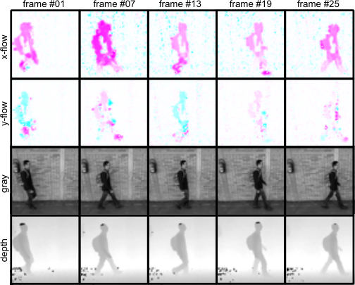
We describe here the different types of modalities used as input for the proposed CNN architecture. In particular, we use optical flow, gray pixels and depth maps since they provide different type of information, are easy to compute and are available in the used datasets. Our intuition is that optical flow will focus on describing the gait-related motion as shown in Castro et al. (2017a), gray pixels are widely used in deep learning Krizhevsky et al. (2012) to encode appearance information and finally depth maps will provide some soft geometric information as commented in Castro et al. (2016). An example of the three types of modalities is represented in Fig. 2.
3.1.1 Optical flow
The use of optical flow (OF) as input data for action representation in video with CNN has already shown excellent results Simonyan and Zisserman (2014). Nevertheless human action is represented by a wide, and usually well defined, set of local motions. In our case, the set of motions differentiating one gait style from another is much more subtle and local.
Let be an OF map computed at time and, therefore, be the value of the OF vector component located at coordinates , where can be either the horizontal or vertical component of the corresponding OF vector. The input data for the CNN are cuboids built by stacking consecutive OF maps , where and corresponds to the value of the horizontal and vertical OF components located at spatial position and time , respectively, ranging in the interval .
Since each original video sequence will probably have a different temporal length, and a CNN requires a fixed size input, we extract subsequences of frames from the full-length sequences. In Fig. 2 we show five frames distributed every six frames along a subsequence of twenty-five frames in total (i.e. frames 1, 7, 13, 19, 25). The first row shows the horizontal component of the OF (-axis displacement) and second row shows the vertical component of the OF (-axis displacement). It can be observed that most of the motion flow is concentrated in the horizontal component, due to the displacement of the person. In order to remove noisy OF located in the background, as it can be observed in Fig. 2, we might think in applying a preprocessing step for filtering out those vectors whose magnitude is out of a given interval. However, since our goal in this work is to minimize the manual intervention in the process of gait signature extraction, we will use those OF maps as returned by the OF algorithm.
3.1.2 Gray-level pixels
When using CNNs for object detection and categorization, the most popular modality is raw pixels Krizhevsky et al. (2012). In contrast to Simonyan and Zisserman (2014), that uses single RGB frames for action recognition, we build cuboids of gray pixels with the aim of better capturing the important features of the subject appearance. Note that in gait recognition, color is not as informative as it is for object recognition. Therefore, using only gray intensity will eventually help CNN to focus just on the gait-relevant information. An example can be seen in the corresponding row of Fig. 2.
3.1.3 Depth maps
As far as we know, the use of depth information has not been explored much in the field of gait recognition. In Hofmann et al. (2014) they basically used depth to segment people from background and compute the Gait Energy Volume descriptor Sivapalan et al. (2011). Castro et al. Castro et al. (2016) represented depth information in a gray-scale image where the intensity of a pixel is the depth value scaled to . In our opinion, depth information is rich and should be studied in depth for this problem. Therefore, given a sequence of depth maps, we extract depth volumes that will be used as input data for the corresponding CNN architecture. An example of depth maps can be seen in the bottom row of Fig. 2.
3.2 CNN architectures for single modality
We have selected the three architectures that most frequently appear in the bibliography and produce state-of-the-art results in different topics (e.g. action recognition, object detection, etc.). The three proposed architectures are: (i) a linear CNN with 2D convolutions (2D-CNN) based on AlexNet Krizhevsky et al. (2012), which is the traditional and most common architecture; (ii) a linear CNN with 3D convolutions and pooling (3D-CNN), which is specially designed to capture information in videos Ji et al. (2012); and, (iii) a 2D very deep residual CNN (ResNet He et al. (2016)), which produces state-of-the-art results in most challenging tasks.
The input to our CNN is a volume of gray pixels, depth maps or OF channels with size for gray and depth, and size for OF since it has two components ( and ). We refer the reader to Sec. 4.2 for the actual values of and used in the experiments. Note that for the case of the 3D CNN on OF, the input must be split into two blocks of size to apply the temporal filters at each OF channel independently, which will be concatenated at deeper layers.
We describe below the four particular models compared in the experimental section (Sec. 4). Note that we use the term ‘softmax layer’ to refer to a fully-connected layer with as many units as classes followed by a softmax exponential layer. Moreover, in all models, the gait signatures are extracted from the layer preceding this softmax layer.
The most common layers of these architectures are the convolutions, pooling and ReLU activation function described in Eq. 1.
| (1) | ||||
where is an input matrix, is an element of that matrix, is a weight of the convolutional filter, is the bias term, is the maximum function and represents the region of where the pooling operation is applied.
2D-CNN: This CNN is composed of the following sequence of layers (Fig. 3a): ‘conv1’, 96 filters of size applied with stride 1 followed by a normalization and max pooling ; ‘conv2’, 192 filters of size applied with stride 2 followed by max pooling ; ‘conv3’, 512 filters of size applied with stride 1 followed by max pooling ; ‘conv4’, 4096 filters of size applied with stride 1; ‘full5’, fully-connected layer with 4096 units and dropout; ‘full6’, fully-connected layer with 2048 units and dropout; and, ‘softmax’, softmax layer with as many units as subject identities. All convolutional layers use the rectification (ReLU) activation function.
3D-CNN: As optical flow has two components and the CNN uses temporal kernels, the network is split into two branches: -flow and -flow. Therefore, each branch contains half of the total filters described below. Then, this CNN is composed by the following sequence of layers (Fig. 3b): ‘conv1’, 96 filters of size applied with stride 1 followed by a max pooling ; ‘conv2’, 192 filters of size applied with stride 2 followed by max pooling ; ‘conv3’, 512 filters of size applied with stride 1 followed by max pooling ; ‘conv4’, 4096 filters of size applied with stride 1; ‘concat’, concatenation of both branches (-flow and -flow); ‘full5’, fully-connected layer with 4096 units and dropout; ‘full6’, fully-connected layer with 2048 units and dropout; and, ‘softmax’, softmax layer with as many units as subject identities. All convolutional layers use the rectification (ReLU) activation function.
ResNet-A: This CNN is composed by the following sequence of layers and residual blocks (a sequences of two convolutions of size , as defined in He et al. (2016) for CIFAR Dataset). This model is specially designed for small datasets with low variability, as this kind of networks tends to overfit due to its high number of layers. As our architecture follows the indications defined by the authors He et al. (2016), we only describe the main blocks (Fig. 3c): ‘conv1’, 16 filters of size applied with stride 1 followed by a max pooling and stride 2; ‘block 1’, 5 residual blocks with convolutions of 16 filters of size applied with stride 1; ‘block 2’, 5 residual blocks with convolutions of 32 filters of size applied with stride 1; ‘block 3’, 5 residual blocks with convolutions of 64 filters of size applied with stride 1; ‘average pooling’, size with stride 1; and, ‘softmax’, softmax layer with as many units as subject identities. All convolutional layers use the rectification (ReLU) activation function and batch normalization.
ResNet-B: This model is an extension of the previous model ResNet-A. The number and size of layers of this model is increased and is specially designed for datasets with high variability (e.g. CASIA-B). This CNN is composed by the following sequence of layers and residual blocks (a sequence of three convolutions of size , and , as defined in He et al. (2016)). As our architecture follows the indications defined by the authors, we only describe the main blocks (Fig. 3d): ‘conv1’, 64 filters of size applied with stride 1 followed by a max pooling and stride 2; ‘block 1’, 4 residual blocks with convolutions of 64 filters of size applied with stride 1; ‘block 2’, 6 residual blocks with convolutions of 128 filters of size applied with stride 1; ‘block 3’, 8 residual blocks with convolutions of 256 filters of size applied with stride 1; ‘block 4’, 3 residual blocks with convolutions of 256 filters of size applied with stride 1; ‘average pooling’, size with stride 1; and, ‘softmax’, softmax layer with as many units as subject identities. All convolutional layers use the rectification (ReLU) activation function and batch normalization.
3.2.1 Model training
For 2D and 3D models, we perform a curriculum learning strategy Bengio et al. (2009) to speed up and to facilitate the convergence. In this learning process, initially, we train a simplified version of each model (i.e. less units per layer and no dropout) and, then, we use the learned network parameters for initializing the layers of a more complex architecture (i.e. 0.1 dropout and more filters and units). This learning process is applied three times until we develop the fourth model. This final model is shown in Fig. 3 and described in the previous section.
During CNN training, the network parameters are learnt using the mini-batch stochastic gradient descent (SGD) algorithm, described in Eq. 2.
| (2) | ||||
where are the trainable parameters of the model, is the learning rate, is the size of the mini-batch, is the output value of the model for the sample, is the label of the sample , is the input sample, is the momentum constant, is the current weights update and is the previous weights update.
In our case, we set momentum equal to in the first two curriculum learning iterations of the 2D and 3D models, and 0.95 during the last one. Note that ResNet-A and ResNet-B are trained from scratch in just one stage (without curriculum learning strategy) so momentum for these networks is set to . We set weight decay to and dropout to (when corresponds). The number of epochs is limited to 20 in TUM-GAID, and the learning rate is initially set to , which is divided by ten when the validation error plateaus. Due to the nature of the ResNet models, the initial learning rate is set to .
In CASIA-B we limit the training stage to 30 epochs, the learning rate is initially set to and it is divided by two when the validation error gets stuck. At each epoch, a mini-batch of 150 samples is randomly selected from a balanced training set (i.e. almost the same proportion of samples per class). Note that for ResNet models we use a mini-batch of 64 samples. When the CNN training has converged, we perform five more epochs on the joint set of training and validation samples.
To run our experiments we use the implementation of CNN provided in MatConvNet library Vedaldi and Lenc (2015). This library allows to develop CNN architectures in an easy and fast manner using the Matlab environment. In addition, it takes advantage of CUDA and cuDNN Chetlur et al. (2014) to improve the performance of the algorithms. Using this open source library will allow other researchers to use our trained models and reproduce our experimental results.
3.2.2 Gait signature evaluation
Once the model is trained, we can extract the gait signatures for a given input. The final stage consists on classifying those signatures to derive a subject identity. Note that, in order to obtain the probabilities from the gait signatures, we use the well-known softmax layer described in Eq. 3.
| (3) |
where is an element of the gait signature.
As it was explained in Sec. 3.1, we split the whole video sequence into overlapping subsequences of a fixed length, and those subsequences are classified independently. Then, we combine the identification results obtained from each subsequence to produce the identification result of the whole video sequence. In our experiments we implement two different strategies for combining subsequence results:
- •
-
SM-Vote. After softmax decision we apply a majority voting strategy on the labels assigned to each subsequence.
- •
-
SM-Prod. The identity is derived from the product of softmax vectors (i.e. probability distributions ) obtained:
(4) where is the number of subsequences extracted from video , is the probability of assigning the identity to the person in video and is the probability of assigning the identity to the person in subsequence .
3.3 Multiple modalities
In this case, we explore different fusion techniques for the signatures extracted from different modalities, expecting that fused information improves the subject identification task.
Late fusion. Focusing on the softmax scores returned by each CNN, we explore the following approaches to combine them: product and weighted sum. These approaches are considered as ‘late fusion’ ones, as fusion is performed on the classification scores.
A) Product of softmax vectors. Given a set of softmax vectors obtained from a set of different modalities , a new score vector is obtained as:
| (5) |
where is the number of modalities used to classify video , can be viewed as the probability of assigning the identity to the person in video and is the probability of assigning the identity to the person in modality .
B) Weighted sum of softmax vectors. Given a set of softmax vectors obtained from a set of different modalities a new score vector is obtained as:
| (6) |
where is the number of modalities used to classify video , can be viewed as the probability of assigning the identity to the person in video , is the probability of assigning the identity to the person in modality and is the weight associated to modality , subject to and .
values are selected empirically by cross-validation. By this way, we have split the training set into training and validation subsets to try different combinations of values. In our case, we have tested all possible values in the range with steps of . Note that the values used for each experiment are specified in its corresponding section. Moreover, the same process is followed during training and test time since we are using late fusion techniques that do not affect the training process.
Early fusion. The fusion performed at gait signature level is known as ‘early fusion’. In our case, as we are working with CNNs, early fusion could be performed at any layer before the ‘softmax’ one. Depending on the layer, the fused descriptors are matrices (fusion before a convolutional layer) or vectors (fusion before a fully-connected layer). We have tried all the possible fusion locations for our CNNs and we have selected the best solution according to the results obtained. In our case, the best early fusion location is after layer ‘full6’ of each modality. The activations of those layers are concatenated and fed into a new set of layers to perform the actual fusion. Therefore, we extend the 2D and 3D networks shown in Fig. 3 with the set of additional layers summarized in Fig. 4:
- ‘concat:’
-
concatenation layer;
- ‘full7:’
-
fully-connected layer with 4096 units, ReLU and dropout;
- ‘full8:’
-
fully-connected layer with 2048 units, ReLU and dropout;
- ‘full9:’
-
fully-connected layer with 1024 units, ReLU and dropout; and,
- ‘softmax:’
-
softmax layer with as many units as subject identities.
During the training process, the parameters of the whole CNN (i.e. the branch of each modality and the fusion layers) are trained altogether, automatically learning the best combination of network parameters for the modalities. At test time, we use the learnt network parameters to fuse the information from the new samples. From our point of view, this kind of fusion is considered early as it is not performed at classification-score level, as done above.
For ResNet models, due to their high number of layers, we do not stack more fully-connected layers to prevent overfitting. Therefore, the selected early fusion architecture is the same as for the rest of models but without fully-connected layers:
- ‘concat:’
-
concatenation layer;
- ‘softmax:’
-
softmax layer with as many units as subject identities and dropout.
4 Experiments and results
We present here the experiments designed to validate our approach and the results obtained on the selected datasets for gait recognition.
4.1 Datasets
We run our experiments on two widely used and challenging datasets for gait recognition: TUM-GAID Hofmann et al. (2014) and CASIA-B Yu et al. (2006). Both datasets are described below.
TUM-GAID. In ‘TUM Gait from Audio, Image and Depth’ (TUM-GAID) 305 subjects perform two walking trajectories in an indoor environment. The first trajectory is performed from left to right and the second one from right to left. Therefore, both sides of the subjects are recorded. Two recording sessions were performed, one in January, where subjects wore heavy jackets and mostly winter boots, and the second in April, where subjects wore different clothes. The action is captured by a Microsoft Kinect sensor which provides a video stream with a resolution of pixels with a frame rate of approximately 30 fps. Some examples can be seen in the left part of Fig. 5 depicting the different conditions included in the dataset.
Hereinafter the following nomenclature is used to refer each of the four walking conditions considered: normal walk (N), carrying a backpack of approximately 5 kg (B), wearing coating shoes (S), as used in clean rooms for hygiene conditions, and elapsed time (TN-TB-TS). Each subject of the dataset is composed of: six sequences of normal walking (N1, N2, N3, N4, N5, N6), two sequences carrying a bag (B1, B2) and two sequences wearing coating shoes (S1, S2). In addition, 32 subjects were recorded in both sessions (i.e. January and April) so they have 10 additional sequences (TN1, TN2, TN3, TN4, TN5, TN6, TB1, TB2, TS1, TS2). Therefore, the overall amount of videos is 3400.
We follow the experimental protocol defined by the authors of the dataset Hofmann et al. (2014). Three subsets of subjects are proposed: training, validation and testing. The training set is used for obtaining a robust model against the different covariates of the dataset. This partition is composed of 100 subjects and the sequences N1 to N6, B1, B2, S1 and S2. The validation set is used for validation purposes and contains 50 different subjects with the sequences N1 to N6, B1, B2, S1 and S2. Finally, the test set contains other 155 different subjects used in the test phase. As the set of subjects is different between the test set and the training set, a new training of the identification model must be performed. For this purpose, the authors reserve the sequences N1 to N4, from the subject test set, to train the model again and the rest of sequences are used for testing and to obtain the accuracy of the model. In the elapsed time experiment, the temporal sequences (TN1, TN2, TN3, TN4, TN5, TN6, TB1, TB2, TS1, TS2) are used instead of the normal ones and the subsets are: 10 subjects in the training set, 6 subjects in the validation set and 16 subjects in the test set.

In our experiments, after parameter selection, the validation sequences are added to the training set for fine-tuning the final model.
CASIA-B. In CASIA-B 124 subjects perform walking trajectories in an indoor environment (right part of Fig. 5). The action is captured from 11 viewpoints (i.e. from to in steps of ) with a video resolution of pixels. Three situations are considered: normal walk (nm), wearing a coat (cl), and carrying a bag (bg). The authors of the dataset indicate that sequences 1 to 4 of the ‘nm’ scenario should be used for training the models. Whereas the remaining sequences should be used for testing: sequences 5 and 6 of ‘nm’, 1 and 2 of ‘cl’ and 1 and 2 of ‘bg’. Therefore, we follow this protocol in our experiments, unless otherwise stated. This makes a total of 496 video sequences for training, per camera viewpoint.
4.2 Implementation details
We ran our experiments on a computer with 32 cores at 2.3 GHz, 256 GB of RAM and a GPU NVidia Titan X Pascal, with MatConvNet library Vedaldi and Lenc (2015) running on Matlab 2016a for Ubuntu 16.04.
For the following experiments with CNN, we resized all the videos to a common resolution of pixels, keeping the original aspect ratio of the video frames. Preliminary experiments support this choice Castro et al. (2017a), as this size exhibits a good trade-off between computational cost and recognition performance. Note that the resolution is 4 times lower than the original CASIA-B one and 8 times lower than the TUM-GAID one.
Given the resized video sequences, we compute dense OF on pairs of frames by using the method of Farneback Farnebäck (2003) implemented in OpenCV library Bradski (2000). In parallel, people are located in a rough manner along the video sequences by background subtraction KaewTraKulPong and Bowden (2002). Then, we crop the video frames to remove part of the background with , obtaining video frames of pixels (full height is kept) and to align the subsequences (people are -located in the middle of the central frame, #13) as in Fig. 2.
Finally, from the cropped OF maps, we build subsequences of frames by stacking OF maps with an overlap of frames. In our case, we chose , that is, to build a new subsequence, we use frames of the previous subsequence and new frames. For most state-of-the-start datasets, 25 frames cover almost one complete gait cycle, as stated by other authors Barnich and Droogenbroeck (2009). Therefore, each OF volume has size .
The same process described above is applied to the gray pixels and depth inputs with values and , obtaining volumes of size . Before feeding the CNN with those data volumes, the mean of the training set for each modality is subtracted to the input data. Both gray and depth values are normalized to the range . Note that in CASIA-B, due to the high variability between viewpoints, it is necessary to normalize gray values to the range .
To increase the amount of training samples we add mirror sequences and apply spatial displacements of pixels in each axis, obtaining a total of 8 new samples from each original sample.
4.3 Performance evaluation
For each test sequence, we return a sorted list of possible identities, where the top one identity corresponds to the largest scored one. According to this we use two quantitative metrics, rank-1 (R1) and rank-5 (R5) accuracy, to measure the performance of the proposed system. Specifically, metric rank-1 measures the percentage of test samples where the top one assigned identity corresponds to the correct one. Metric rank-5 measures the percentage of test samples where the ground truth identity is included in the first five ranked identities for the corresponding test sample. Note that rank-5 is less strict than rank-1 and, in a real system, it would allow to verify if the target subject is any of the top five most probably ones. In order to compute the accuracy metric, we use the general equation:
| (7) |
where the numerator indicates the number of correct predictions and the denominator specifies the total number of predictions.
4.4 Experimental results on TUM-GAID
In this section, we work with TUM-GAID dataset to evaluate the impact of CNN architectures in automatic extraction of gait signatures from diverse modalities, studying which one is the most convenient for the different scenarios. Afterwards, we evaluate the impact of combining gait signatures from different modalities for people identification. Finally, we compare our results with the state-of-the-art ones.
4.4.1 Single modality evaluation
In this experiment, we evaluate the individual contribution of each input modality (i.e. gray pixels, optical flow and depth maps) and each architecture (i.e. 2D, 3D and ResNet) for extracting discriminative gait signatures. We apply the metrics explained above (Sec. 4.3). Note that, as this dataset only contains a single viewpoint, ResNet models tend to overfit due to the lack of variability in the training data. Therefore, we use ResNet-A (see Sec. 3.2 for more details) which is a shallower model designed for smaller datasets than the default ResNet models. Tab 2 summarizes the identification results obtained on TUM-GAID with each modality: Gray, OF and Depth. Each column contains the results for rank-1 (R1) and rank-5 (R5) for each scenario. The last column ‘AVG’ is the average of each case (temporal and non temporal) weighted by the number of classes.
Focusing on the average results, we can see that the best R1 results are obtained by the 3D-CNN using OF modality. This clearly shows the importance of the temporal information captured by the 3D convolutions and the relevance of the motion information provided by the OF. Regarding the best R5 result, it is obtained by the 2D-CNN using again the OF modality. For this metric, the 2D-CNN produces better results than the others architectures showing the robustness of this model, i.e. it is able to include the correct identity in the top-5 predictions more times than the other models. Finally, note that the two strategies employed for obtaining the identity at video level, SM-Vote and SM-Prod, offer similar performance. However, SM-Prod seems to work slightly better in terms of average R1.
| N | B | S | TN | TB | TS | AVG | ||||||||||
|---|---|---|---|---|---|---|---|---|---|---|---|---|---|---|---|---|
| R1 | R5 | R1 | R5 | R1 | R5 | R1 | R5 | R1 | R5 | R1 | R5 | R1 | R5 | |||
| 2D-CNN | Gray | SM-Vote | 99.4 | 100 | 99.0 | 99.7 | 98.4 | 99.7 | 31.3 | 53.1 | 34.4 | 65.6 | 34.4 | 62.5 | 92.8 | 96.1 |
| SM-Prod | 100 | 100 | 99.7 | 99.7 | 98.4 | 99.7 | 28.1 | 62.5 | 37.5 | 71.9 | 34.4 | 59.4 | 93.2 | 96.5 | ||
| OF | SM-Vote | 99.4 | 100 | 97.4 | 100 | 96.4 | 99.4 | 53.1 | 96.9 | 43.8 | 87.5 | 56.3 | 93.8 | 93.4 | 99.1 | |
| SM-Prod | 99.4 | 100 | 97.7 | 100 | 96.1 | 99.4 | 56.3 | 87.5 | 43.8 | 84.4 | 59.4 | 90.6 | 93.6 | 98.7 | ||
| Depth | SM-Vote | 98.4 | 100 | 65.8 | 90.0 | 96.8 | 99.7 | 34.4 | 93.8 | 34.4 | 93.8 | 50.0 | 84.4 | 82.6 | 96.0 | |
| SM-Prod | 98.7 | 100 | 66.1 | 90.7 | 96.8 | 99.7 | 43.8 | 90.6 | 40.6 | 87.5 | 46.8 | 84.4 | 83.1 | 95.9 | ||
| 3D-CNN | Gray | SM-Vote | 99.7 | 100 | 98.4 | 99.7 | 96.8 | 99 | 21.9 | 50 | 21.9 | 46.9 | 12.5 | 43.8 | 90.9 | 94.6 |
| SM-Prod | 97.7 | 97.7 | 93.9 | 94.2 | 91.3 | 91.6 | 18.8 | 37.5 | 21.9 | 37.5 | 12.5 | 31.3 | 87.1 | 89 | ||
| OF | SM-Vote | 99 | 99.4 | 95.5 | 99.7 | 94.2 | 98.1 | 65.6 | 90.6 | 65.6 | 93.8 | 59.4 | 87.5 | 93.2 | 98.3 | |
| SM-Prod | 98.7 | 99.7 | 97.1 | 99.4 | 94.5 | 98.7 | 71.9 | 87.5 | 68.8 | 87.5 | 65.6 | 84.4 | 94.1 | 98.1 | ||
| Depth | SM-Vote | 97.7 | 98.4 | 84.2 | 96.5 | 96.8 | 99.4 | 68.8 | 100 | 50 | 100 | 75 | 100 | 90.3 | 98.3 | |
| SM-Prod | 98.4 | 100 | 86.8 | 96.1 | 97.4 | 99.4 | 62 | 87.4 | 53.1 | 96.9 | 78.1 | 100 | 91.4 | 98.2 | ||
| RESNET-A | Gray | SM-Vote | 99.4 | 100 | 95.8 | 99.4 | 96.1 | 99 | 25 | 62.5 | 34.4 | 98.8 | 25 | 59.4 | 90.6 | 96.1 |
| SM-Prod | 99 | 100 | 96.5 | 99.4 | 95.5 | 99 | 28.1 | 56.3 | 34.4 | 68.8 | 25 | 56.3 | 90.7 | 95.8 | ||
| OF | SM-Vote | 94.5 | 99.7 | 81 | 98.4 | 85.1 | 97.7 | 34.4 | 93.8 | 34.4 | 90.6 | 37.5 | 93.8 | 82.1 | 98.1 | |
| SM-Prod | 95.2 | 99.4 | 81 | 98.7 | 86.1 | 97.7 | 34.4 | 96.7 | 40.6 | 93.8 | 43.8 | 93.8 | 83 | 98.2 | ||
| Depth | SM-Vote | 77.7 | 99.4 | 60 | 91.6 | 71.8 | 97.4 | 56.3 | 81.3 | 37.5 | 81.3 | 46.9 | 90.6 | 67.7 | 95 | |
| SM-Prod | 77.1 | 98.4 | 60 | 91.3 | 70.9 | 96.1 | 56.3 | 78.1 | 34.4 | 81.3 | 46.9 | 87.5 | 67.1 | 94.1 | ||
In order to compare the performance of the different models and modalities per scenario (i.e. temporal and non-temporal), we summarize the most important results of Tab. 2 in Fig. 6. It shows the best R1 average performance for non-temporal and temporal scenarios per modality. If we focus on the non-temporal scenarios (N, B and S), we can see gait signatures based on Gray are able to outperform the results obtained with OF. In our opinion, appearance models have such a good performance due to the low appearance variability of this scenario. On the other hand, if we focus on the temporal scenarios (TN, TB and TS), the worst results are obtained with Gray. These results evidence the weakness of appearance models under conditions with high variability between training and test samples (like our temporal experiment). However, OF models have a better sturdiness against appearance changes on the inputs. With regard to the type of architecture, the behaviour of all of them is very similar on the non-temporal scenarios, where the best results are obtained by the 2D-CNN using Gray as input, followed by the 3D-CNN with Gray. However, for the temporal scenarios, 3D-CNN offers its best results in using either OF or Depth, whereas 2D-CNN and ResNet work better with Gray. Considering the average accuracy over all the scenarios, 2D-CNN works better with Gray, and 3D-CNN with both OF and Depth.
Thus, we can conclude that the best architectures for this task are 2D-CNN and 3D-CNN, and the best modalities are Gray for the non-temporal scenario and OF for the temporal scenario.
| OF-Gray | OF-Depth | All | |||||||||||||
|---|---|---|---|---|---|---|---|---|---|---|---|---|---|---|---|
| P1 | P2 | P3 | P4 | P5 | P1 | P2 | P3 | P4 | P5 | P1 | P2 | P3 | P4 | P5 | |
| 2D-CNN | 90.7 | 91.9 | 91.8 | 93.9 | 93.8 | 81.8 | 92.7 | 91.9 | 92.2 | 93.1 | 86.4 | 90.1 | 92.8 | 93.5 | 93.9 |
| 3D-CNN | 92.3 | 91.3 | 89.4 | 92.7 | 92.9 | 86.6 | 78.6 | 71.8 | 89.0 | 89.2 | 87.9 | 82.5 | 87.3 | 92.2 | 92.7 |
| ResNet | 86.8 | 89.4 | 89.3 | 92.4 | 92.6 | 83.2 | 83.1 | 85.5 | 90.4 | 90.0 | 84.7 | 87.8 | 88.2 | 92.9 | 90.6 |
4.4.2 Multiple modality evaluation
As we can use three types of modalities from TUM-GAID, we study here the benefits of fusing information from different modalities. In this section, we compare the baseline obtained by each single modality with our two late fusion approaches, which are performed at score level, and our early fusion approach, which is performed at gait signature level. For more details about our fusion approaches (early and late methods), please see Sec. 3.3. Since there are many combinations of modalities, our experiments focus just on the combinations that include optical flow due to the sturdiness of this modality under all walking conditions.
Note that, in this section, the data of Tab. 2 are used as baseline case, concretely, data obtained with the product of softmax vectors on each modality.
Focusing on the early fusion approach, we have studied the impact of fusion on network performance attending to the position where fusion is applied in the architecture. Thus, Tab. 3 summarizes the average results of three trials per network for five different fusion positions. For 2D-CNN and 3D-CNN, the positions P1 to P4 refer to the convolutional layers and P5 allude to the fully-connected layer. For RestNet, P1 to P4 correspond to the last convolutional layer of each residual block and P5 is the average pooling layer. Focusing on the results, we can see that for 2D-CNN and 3D-CNN, the best results are obtained in the last fusion position. For ResNet, P4 and P5 achieve similar results in most of the cases, so we are going to focus on P5 since this layer produces an uni-dimensional feature vector which does not requires any further pre-processing in order to be used by our fusion approaches. Note that in the following tables, the early fusion results are selected from the best position and the best of the three trials.
Now, we analyse the fusion results within each type of architecture. The results of Tab. 4 correspond to 2D-CNN and indicate that, in general, the best option is to combine all three modalities for all fusion methods except for SM Prod where it is better to use only OF and Gray. Note that for Weighted Sum, we have used the weights and for OF, Gray and Depth, respectively, when we fuse all modalities. In the case of only two modalities, we use fusion weights and for OF and the other modality, respectively. According to the results, in the non temporal scenarios we only improve the results with respect to the single modalities in scenario S, while in the other scenarios we obtain similar results (since they are higher than , the improvement is very difficult). Regarding the fusion strategy, the proposed Early fusion CNN provides on average the best results showing that it is better to combine the information from multiple modalities during the training process. By this way, the parameters of the network are able to learn the best combination that maximizes the accuracy.
| Fusion | Modalities | N | B | S | TN | TB | TS | AVG |
|---|---|---|---|---|---|---|---|---|
| Single | Gray | 100 | 99.7 | 98.4 | 28.1 | 37.5 | 34.4 | 93.2 |
| OF | 99.4 | 97.7 | 96.1 | 56.3 | 43.8 | 59.4 | 93.6 | |
| Depth | 98.7 | 66.1 | 96.8 | 43.8 | 40.6 | 46.8 | 83.1 | |
| SM Prod | OF-Gray | 99.7 | 99.7 | 99.0 | 40.6 | 37.5 | 53.1 | 94.3 |
| OF-Depth | 92.9 | 88.1 | 98.7 | 59.4 | 40.6 | 46.9 | 89.1 | |
| All | 92.9 | 90.0 | 99.0 | 56.3 | 56.3 | 50.0 | 90.2 | |
| W. Sum | OF-Gray | 99.4 | 98.4 | 98.7 | 50.0 | 34.4 | 53.1 | 93.9 |
| OF-Depth | 97.7 | 93.9 | 99.0 | 53.1 | 43.8 | 59.4 | 92.7 | |
| All | 99.0 | 98.1 | 99.7 | 50.0 | 34.4 | 53.1 | 94.0 | |
| Early | OF-Gray | 99.4 | 98.7 | 97.7 | 56.3 | 43.8 | 43.8 | 93.9 |
| OF-Depth | 99.0 | 96.1 | 96.4 | 53.1 | 53.1 | 46.9 | 92.9 | |
| All | 99.4 | 98.4 | 98.7 | 56.3 | 53.1 | 46.9 | 94.5 |
Focusing on the results obtained with the 3D-CNN (Tab. 5), the best average accuracy is reported by the combination of all modalities by W Sum. However, it is only slightly better than the best result obtained by using only OF. Due to the low accuracy obtained with Gray, combining it with other features worsen the fused results.
| Fusion | Modalities | N | B | S | TN | TB | TS | AVG |
| Single | Gray | 97.7 | 93.9 | 91.3 | 18.8 | 21.9 | 12.5 | 87.1 |
| OF | 98.7 | 97.1 | 94.5 | 71.9 | 68.8 | 65.6 | 94.1 | |
| Depth | 98.4 | 86.8 | 97.4 | 62 | 53.1 | 78.1 | 91.4 | |
| SM Prod | OF-Gray | 93.5 | 84.8 | 83.5 | 12.5 | 12.5 | 15.6 | 80.4 |
| OF-Depth | 92.2 | 97.4 | 96.8 | 78.1 | 62.5 | 15.6 | 91.4 | |
| All | 78.4 | 84.2 | 83.5 | 12.5 | 21.9 | 12.5 | 75.8 | |
| W. Sum | OF-Gray | 97.4 | 98.1 | 96.1 | 71.9 | 50 | 53.1 | 93.6 |
| OF-Depth | 95.5 | 96.5 | 96.8 | 65.6 | 68.8 | 53.1 | 93.1 | |
| All | 96.8 | 98.4 | 97.1 | 65.6 | 65.6 | 59.4 | 94.3 | |
| Early | OF-Gray | 99.4 | 96.8 | 94.5 | 62.5 | 50 | 56.3 | 93.1 |
| OF-Depth | 84.8 | 97.4 | 97.4 | 71.9 | 68.8 | 71.9 | 91.1 | |
| All | 99.7 | 98.7 | 97.7 | 34.4 | 25 | 31.3 | 92.3 |
Finally, the ResNet architecture (see Tab. 6) shows unexpected low fusion results. It may indicate that the probability distribution on the classes obtained at the softmax layer does not show clearly defined maxima, and small changes in those values cause important changes in the final classes. However, Early Fusion improves the results on average for the combination OF and Gray, what indicates that adding more inputs to the training process can be beneficial to avoid local minima.
In summary, by using multimodal information the recognition accuracy improves with respect to the best single modality (i.e. OF).
| Fusion | Modalities | N | B | S | TN | TB | TS | AVG |
| Single | Gray | 99.0 | 96.5 | 95.5 | 28.1 | 34.4 | 25.0 | 90.7 |
| OF | 95.2 | 81.0 | 86.1 | 37.5 | 40.6 | 43.8 | 83.1 | |
| Depth | 77.1 | 60.0 | 71.0 | 56.3 | 34.4 | 46.9 | 67.2 | |
| SM Prod | OF-Gray | 84.8 | 77.7 | 79.3 | 46.9 | 40.6 | 50 | 77.3 |
| OF-Depth | 71.2 | 63.6 | 69.6 | 53.1 | 37.5 | 53.1 | 66.2 | |
| All | 79.9 | 80.7 | 81.9 | 56.3 | 34.4 | 56.3 | 77.9 | |
| W. Sum | OF-Gray | 72.8 | 60.7 | 64.4 | 31.3 | 31.3 | 40.6 | 63 |
| OF-Depth | 68.3 | 53.9 | 62.5 | 37.5 | 46.9 | 56.3 | 60.2 | |
| All | 72.5 | 60 | 64.7 | 31.3 | 28.1 | 46.9 | 62.9 | |
| Early-RES | OF-Gray | 99.4 | 94.8 | 97.7 | 40.6 | 34.4 | 43.8 | 91.9 |
| OF-Depth | 95.8 | 93.2 | 96.1 | 40.6 | 37.5 | 43.8 | 89.9 | |
| All | 80.3 | 87.1 | 88.4 | 40.6 | 50 | 50 | 81.7 |
4.4.3 State-of-the-art on TUM-GAID
In Tab. 7, we compare our results with the state-of-the-art in TUM-GAID under all modalities previously employed (Gray, OF, Depth and Fusion). First of all, we would like to remark that our approach uses a resolution of while the rest of the methods use . Therefore, our method uses times less information. If we focus on the visual modality (Gray in our case), we can see that our method outperforms previous results in non temporal scenarios establishing a new state-of-the-art . On the other hand, in the temporal scenarios we have lower results than the other methods due to the high variability in visual information. Then, if we focus on OF, we can see that the best results are obtained by PFM Castro et al. (2017) with a resolution of . Nevertheless, if we apply PFM with a resolution of , its results worsen dramatically and our CNN is able to outperform it in all scenarios. If we compare our CNN with other deep learning approaches presented in the literature, only MTaskCNN-7NN Marín-Jiménez et al. (2017) is able to improve our approach. This model has been trained in a multi-task fashion so, during training, there are more information available to optimize the network parameters. If we focus on the other deep learning approaches, we can see that we obtain similar results (only a lower) on average but, we obtain the state-of-the-art for temporal scenario. In Depth modality, we can see that our method obtains better results than other methods, which use full resolution frames, in all cases except N. Nevertheless, on average, we are able to obtain more than a of improvement. Finally, if we fuse information from all modalities with a CNN, the average score achieved by both scenarios (temporal and non-temporal) beats all the methods shown in Tab. 7 with the exception of PFM (640x480) Castro et al. (2017) and MTaskCNN-7NN Marín-Jiménez et al. (2017), where we are and below, respectively. However, if we apply the same 7NN approach as in Marín-Jiménez et al. (2017), and we fuse the probabilities obtained, we set a new state-of-the-art ( vs ) for all scenarios with our 3D-CNN-7NN-All using Softmax Product as fusion.
| Modality | Input Size | Method | N | B | S | Avg | TN | TB | TS | Avg | Global Avg |
| Visual Data | SDL Zeng et al. (2014) | - | - | - | - | 96.9 | - | - | - | - | |
| GEI Hofmann et al. (2014) | 99.4 | 27.1 | 52.6 | 59.7 | 44.0 | 6.0 | 9.0 | 19.7 | 56.0 | ||
| SEIM Whytock et al. (2014) | 99.0 | 18.4 | 96.1 | 71.2 | 15.6 | 3.1 | 28.1 | 15.6 | 66.0 | ||
| GVI Whytock et al. (2014) | 99.0 | 47.7 | 94.5 | 80.4 | 62.5 | 15.6 | 62.5 | 46.9 | 77.3 | ||
| SVIM Whytock et al. (2014) | 98.4 | 64.2 | 91.6 | 84.7 | 65.6 | 31.3 | 50.0 | 49.0 | 81.4 | ||
| RSM Guan and Li (2013) | 100 | 79.0 | 97.0 | 92.0 | 58.0 | 38.0 | 57.0 | 51.0 | 88.2 | ||
| Gray | 2D-CNN-SMP (ours) | 100 | 99.7 | 98.4 | 99.4 | 28.1 | 37.5 | 34.4 | 33.3 | 93.2 | |
| OF | PFM Castro et al. (2017) | 99.7 | 99.0 | 99.0 | 99.2 | 78.1 | 62.0 | 54.9 | 65.0 | 96.0 | |
| PFM Castro et al. (2017) | 75.8 | 70.3 | 32.3 | 59.5 | 50.0 | 40.6 | 25.0 | 38.5 | 57.5 | ||
| OF-CNN-NN Castro et al. (2017a) | 99.7 | 98.1 | 95.8 | 97.9 | 62.5 | 56.3 | 59.4 | 59.4 | 94.3 | ||
| OF-ResNet-B Castro et al. (2017b) | 99 | 95.5 | 97.4 | 97.3 | 65.6 | 62.5 | 68.8 | 65.6 | 94.3 | ||
| MTaskCNN-7NN Marín-Jiménez et al. (2017) | 99.7 | 97.4 | 99.7 | 98.9 | 59.4 | 62.5 | 68.8 | 63.6 | 95.6 | ||
| 3D-CNN-SMP (ours) | 98.7 | 97.1 | 94.5 | 96.8 | 71.9 | 68.8 | 65.6 | 68.8 | 94.1 | ||
| Depth | DGHEI Hofmann et al. (2014) | 99.0 | 40.3 | 96.1 | 78.5 | 50.0 | 0.0 | 44.0 | 31.3 | 74.1 | |
| 3D-CNN-SMP (ours) | 98.4 | 86.8 | 97.4 | 94.2 | 62.0 | 53.1 | 78.1 | 64.4 | 91.4 | ||
| Fusion | DGHEI + GEI Hofmann et al. (2014) | 99.4 | 51.3 | 94.8 | 81.8 | 66.0 | 3.0 | 50.0 | 39.7 | 77.9 | |
| 2D-CNN-All (ours) | 99.4 | 98.4 | 98.7 | 98.8 | 56.3 | 53.1 | 46.9 | 52.1 | 94.5 | ||
| 3D-CNN-7NN-All (ours) | 100 | 99.4 | 99.4 | 99.6 | 75 | 62.5 | 62.5 | 66.7 | 96.5 |
4.5 Experimental results on CASIA-B
We focus here on CASIA-B dataset, which offers different covariate factors and multiple viewpoints. Note that, for the sake of comparison with other methods, we train our models with all cameras and we test them both on the camera, as done in the state-of-the-art approaches Wu et al. (2017); Castro et al. (2017), and on all cameras like in Wu et al. (2017).
4.5.1 Single modality evaluation
As this dataset contains eleven viewpoints, ResNet models have enough variability in the training data. Therefore, we use ResNet-B (see Sec. 3.2 for more details) which is deeper than ResNet-A. Tabs. 8 and 9 summarize the identification results obtained on CASIA-B and multicamera setup, respectively, for each modality: Gray and OF. Note that this dataset does not provide depth information. R1 and R5 columns contain the results for rank-1 (R1) and rank-5 (R5) for each scenario. The last column ‘AVG’ is the average of all scenarios. The results at sequence level are obtained by multiplying the scores of the softmax layer. Note that as in CASIA-B there is no training partition to build the model, we have split the dataset into a training set composed of the first 74 subjects and a test set composed of the 50 remaining subjects, following the indications in Wu et al. (2017). During the training process, all viewpoints and training samples are used.
| nm | bg | cl | AVG | |||||||
|---|---|---|---|---|---|---|---|---|---|---|
| R1 | R5 | R1 | R5 | R1 | R5 | R1 | R5 | |||
| Gray | 2D | SM-Vote | 91 | 98 | 82 | 95 | 37 | 82 | 70 | 91.7 |
| SM-Prod | 92 | 100 | 85 | 98 | 45 | 90 | 74 | 96 | ||
| 3D | SM-Vote | 72 | 93 | 69 | 87 | 33 | 76 | 58 | 85.3 | |
| SM-Prod | 81 | 92 | 73 | 90 | 45 | 77 | 66.3 | 86.3 | ||
| RES | SM-Vote | 94 | 100 | 89 | 98 | 42 | 83 | 75 | 93.7 | |
| SM-Prod | 96 | 100 | 91 | 98 | 46 | 98 | 77.7 | 98.7 | ||
| OF | 2D | SM-Vote | 99 | 99 | 76 | 90 | 28 | 51 | 67.7 | 80 |
| SM-Prod | 99 | 99 | 78 | 93 | 27 | 62 | 68 | 84.7 | ||
| 3D | SM-Vote | 98 | 99 | 86 | 99 | 37 | 70 | 73.7 | 89.3 | |
| SM-Prod | 98 | 100 | 88 | 98 | 36 | 67 | 74 | 88.3 | ||
| RES | SM-Vote | 94 | 100 | 83 | 98 | 47 | 73 | 74.7 | 90.3 | |
| SM-Prod | 93 | 100 | 85 | 98 | 46 | 71 | 74.7 | 89.7 | ||
| nm | bg | cl | AVG | |||||||
|---|---|---|---|---|---|---|---|---|---|---|
| R1 | R5 | R1 | R5 | R1 | R5 | R1 | R5 | |||
| Gray | 2D | SM-Vote | 97.1 | 99.6 | 89.8 | 98.5 | 38.4 | 78.7 | 75.1 | 92.3 |
| SM-Prod | 98.3 | 100 | 91.5 | 99.2 | 40.4 | 77.2 | 76.7 | 92.1 | ||
| 3D | SM-Vote | 92.7 | 98.8 | 87.1 | 96.3 | 43.9 | 72.8 | 74.6 | 89.3 | |
| SM-Prod | 96.1 | 99.1 | 88.7 | 96.9 | 47.0 | 71.7 | 77.3 | 89.2 | ||
| RES | SM-Vote | 99.2 | 100 | 91.6 | 99.4 | 44.1 | 78.4 | 78.3 | 92.6 | |
| SM-Prod | 99.5 | 100 | 92.3 | 99.6 | 45.6 | 78.6 | 79.1 | 92.7 | ||
| OF | 2D | SM-Vote | 97.6 | 99.7 | 82.4 | 95.5 | 38.3 | 63.9 | 72.8 | 86.4 |
| SM-Prod | 97.6 | 99.8 | 83.4 | 96.3 | 37.9 | 68.5 | 73.0 | 88.2 | ||
| 3D | SM-Vote | 98.2 | 99.8 | 89.7 | 99.1 | 45.0 | 78.2 | 77.6 | 92.4 | |
| SM-Prod | 98.4 | 99.9 | 90.5 | 98.8 | 45.1 | 76.7 | 78.0 | 91.8 | ||
| RES | SM-Vote | 95.9 | 100 | 84.9 | 98.7 | 47.4 | 83.1 | 76.1 | 93.9 | |
| SM-Prod | 96.0 | 100 | 86.7 | 98.5 | 48.0 | 79.9 | 76.9 | 92.8 | ||
According to the results obtained for the view-point and for all cameras, we can see that our model is able to identify people with a high accuracy in scenarios nm and bg while in scenario cl we have lower precision due to the high appearance changes. If we focus on the modality used, on average, Gray is the best option most of the time. In this dataset, with huge variations between points of view, the shape of the subject seems to be important and it helps to classification. In scenario cl our models experiment a huge decrease in accuracy mainly caused by the high variability of coats worn by the subjects. This can be seen in Fig. 5 on the right part of the last row. In these pictures, the coat occludes the legs and if we add the fact that we have different kind of coats with different number of occurrences, our CNN is not able to learn good features for this scenario due to the high variability and low number of samples.
On the other hand, for this dataset, OF seems that it is not able to find a good representation if the shape of the subject changes drastically. We think that this is because of the high variability in the appearance of the subjects seen from the different cameras used for training. Therefore, as the models receive different flow vectors, the training process cannot produce a view-independent model and the global performance decreases. For example, frontal-views produce vectors whose main movement is focused on Y-axis (there is no horizontal displacement of the subject) while lateral-views produce vectors whose movement is focused on X-axis.
If we analyze the average recognition percentage achieved by the different architectures, it is clear that ResNet-B obtains the best results for all modalities with the camera. When all cameras are used for testing, ResNet-B obtains the best results for Gray modality while 3D-CNN achieves the best results for OF. That shows that ResNet is the most powerful model when data with enough variability is available. On the other hand, 3D-CNN obtains good results for the OF modality, while 2D-CNN achieves good results for the Gray modality.
Thus, we can conclude that the best architecture for this dataset is ResNet, and the best modalities are Gray for R1 metric and OF for R5 metric.
4.5.2 Multiple modality evaluation
In this dataset only two modalities are available (i.e. gray and OF) so fusion experiments are restricted to just both of them. As we have done for TUM-GAID dataset, we compare the baseline obtained by each single modality with our two late fusion approaches, which are performed at score level, and our early fusion approach, which is performed at gait signature level. Again, in this section, the data of Tabs. 8 and 9 are used as baseline case, concretely, data obtained with the product of softmax vectors on each modality.
It can be observed in Tabs. 10 and 11 that the best method for fusing Gray and OF modalities is, on average, Softmax product followed by weighted sum (with weights and for Gray and OF, respectively). Focusing on the three architectures, ResNet obtains the best fusion results for the camera while 2D-CNN achieves the best results using all cameras.
In this case, early fusion is not able to improve the single modality results. In our opinion, this is due to high variability between viewpoints. In addition, we have observed that the two branches of the network have different convergence speeds, hence the final features are not fused properly producing bad representations.
Thus, in this dataset, the late fusion (SM-Prod) improves the single modality results showing that both modalities are complementary and the combination of both boosts the performance of the models. Moreover, the boost is very significant in many cases with improvements higher than (e.g. ResNet with all cameras).
| 2D-CNN | 3D-CNN | ResNet | ||||||||||
| nm | bg | cl | AVG | nm | bg | cl | AVG | nm | bg | cl | AVG | |
| Gray | 92 | 85 | 45 | 74 | 81 | 73 | 45 | 66.3 | 96 | 91 | 46 | 77.7 |
| OF | 99 | 78 | 27 | 68 | 98 | 88 | 36 | 74 | 93 | 85 | 46 | 74.7 |
| SM-Prod | 99 | 95 | 41 | 78.3 | 98 | 96 | 49 | 81 | 98 | 97 | 63 | 86 |
| W. Sum | 99 | 94 | 39 | 77.3 | 98 | 95 | 46 | 79.7 | 98 | 96 | 60 | 84.7 |
| Early | 83 | 61 | 26 | 56.7 | 76 | 74 | 46 | 65.3 | 67 | 63 | 38 | 56 |
| 2D-CNN | 3D-CNN | ResNet | ||||||||||
| nm | bg | cl | AVG | nm | bg | cl | AVG | nm | bg | cl | AVG | |
| Gray | 98.3 | 91.5 | 40.4 | 76.7 | 96.1 | 88.7 | 47.0 | 77.3 | 99.5 | 92.3 | 45.6 | 79.1 |
| OF | 97.6 | 83.4 | 37.9 | 73.0 | 98.4 | 90.5 | 45.1 | 78.0 | 96.0 | 86.7 | 48.0 | 76.9 |
| SM-Prod | 99.8 | 96.1 | 67.0 | 87.6 | 99.7 | 97.4 | 54.9 | 84.0 | 99.7 | 96.7 | 59.1 | 85.2 |
| W. Sum | 99.7 | 95.8 | 66.6 | 87.4 | 99.7 | 97.2 | 52.8 | 83.2 | 99.7 | 96.4 | 56.9 | 84.3 |
| Early | 76.2 | 63.8 | 30.2 | 56.7 | 70.5 | 68.2 | 41.1 | 59.9 | 68.7 | 64.8 | 37.1 | 56.9 |
4.5.3 State-of-the-art on CASIA-B
In Tabs. 12 and 13, we compare our results with the state-of-the-art in CASIA-B under all modalities used before (Gray and OF) and their fusion. First of all, we would like to remark that our approach uses a resolution of while the rest of methods use . Therefore, our method uses times less information. Regarding OF with the 90°camera, the best results are obtained by PFM Castro et al. (2017) with a resolution of . Nevertheless, if we apply it with a resolution of , its results worsen dramatically and our ResNet-B is able to outperform it in all scenarios. With this modality, our model sets the second best result in the state-of-the-art (apart from PFM with full resolution). Using all cameras, the best results are achieved by the proposed 3D-CNN although in this case, there are no other approaches to compare with. If we focus on the visual modality (Gray in our case) for the 90°camera and all cameras, we can see that L-CRF Chen et al. (2018) achieves the best results with a resolution of . However, as this approach is based on dense trajectories, smaller resolutions should produce worse results as we have seen in PFM, which is also based on dense trajectories. For this modality, our best results are obtained by ResNet-B. Finally, our fusion (softmax product) obtains the best result and it improves our ResNet-B for 90°camera using Gray modality by a . In the case of using all cameras, our softmax product also improves the results with 2D-CNN by a .
Comparing our method with Wu et al. (2017), which is the closest approach to ours as they also employ CNNs, our best average result improves a for the 90°camera and a for all cameras with respect to their best average accuracy. Focusing on individual scenarios, they only improve our results in cl scenario if we use a single modality, probably due to the use of a gallery-probe scheme, i.e., at test time, they must compare the test sample with all the probe samples to get all distances, then, they select the class of the probe sample with the lowest distance. This method is slower than our approach where we only need to propagate the test sample through the CNN to obtain the class. In addition, if we use our fusion approach, our approach improves them in all scenarios.
| Modality | Input Size | Method | #subjs | #train | #test | nm | bg | cl | Avg |
| Visual Data | GEI Yu et al. (2006) | 124 | 4 | 2 | 97.6 | 52.0 | 32.7 | 67.8 | |
| GEI Yu et al. (2006) | 124 | 4 | 2 | 97.6 | 52.0 | 32.7 | 67.8 | ||
| iHMM Hu et al. (2013) | 84 | 5 | 1 | 94.0 | 45.2 | 42.9 | 60.7 | ||
| CGI Wang et al. (2012) | 124 | 1 | 1 | 88.1 | 43.7 | 43.0 | 58.3 | ||
| SDCNN Alotaibi and Mahmood (2015) | 124 | 4 | 2 | 95.6 | - | - | - | ||
| GSP-CTC Li et al. (2018) | 124 | 4 | 2 | 99.2 | 77.2 | 73.0 | 83.1 | ||
| L-CRF Chen et al. (2018) | 100 | 4 | 2 | 98.6 | 90.2 | 85.8 | 91.5 | ||
| DCNN Wu et al. (2015) | 124 | 4 | 2 | 81.5 | - | - | - | ||
| LBCNN Wu et al. (2017) | 50 | 4 | 2 | 91.5 | 63.1 | 54.6 | 69.7 | ||
| Gray | ResNet-B (ours) | 50 | 4 | 2 | 96.0 | 91.0 | 46.0 | 77.7 | |
| OF | PFM Castro et al. (2017) | 124 | 4 | 2 | 100 | 100 | 85.5 | 95.2 | |
| PFM Castro et al. (2017) | 124 | 4 | 2 | 88.3 | 66.5 | 44.0 | 66.3 | ||
| ResNet-B (ours) | 50 | 4 | 2 | 93.0 | 85.0 | 46.0 | 74.7 | ||
| Fusion | ResNet-B-SMP (ours) | 50 | 4 | 2 | 98.0 | 97.0 | 63.0 | 86.0 |
| Modality | Input Size | Method | #subjs | #train | #test | nm | bg | cl | Avg |
|---|---|---|---|---|---|---|---|---|---|
| Visual Data | LBCNN Wu et al. (2017) | 50 | 4 | 2 | 94.1 | 72.4 | 54.0 | 73.5 | |
| Gray | ResNet-B (ours) | 50 | 4 | 2 | 99.5 | 92.3 | 45.6 | 79.1 | |
| OF | 3D-CNN (ours) | 50 | 4 | 2 | 98.4 | 90.5 | 45.1 | 78.0 | |
| Fusion | 2D-CNN-SMP (ours) | 50 | 4 | 2 | 99.8 | 96.1 | 67.0 | 87.6 |
4.6 Released material
In order to make reproducible the experimental results obtained in this paper,
the CNN models obtained during the experiments have been publicly released for the research community at the following website:
https://github.com/avagait/cnngaitmm
After the review process, we also plan to release the related source code for reproducing the experiments.
5 Conclusions
We have presented a comparative study of multimodal systems based on CNN architectures for the problem of people identification based on the way the walk (i.e. gait recognition). The evaluated architectures are able to extract automatically gait signatures from sequences of gray pixels, optical flow and depth maps. Those gait signatures have been tested on the task of people identification, obtaining state-of-the-art results on two challenging datasets, i.e. TUM-GAID and CASIA-B, that cover diverse scenarios (e.g. people wearing long coats, carrying bags, changing shoes or camera viewpoint changes).
With regard to the type of input modalities, we may conclude that, under similar viewpoints (e.g. TUM-GAID) the weakest one is gray pixels, as it is highly appearance dependant. However, as it could be expected optical flow is the one that better encodes body motion. Depth maps work fairly well if changes in appearance are small (i.e. shoes scenario). In datasets with multiple viewpoints (e.g. CASIA-B), gray pixels achieve the best results, probably due to optical flow produces extremely different vectors depending on the viewpoint so, during training, the optimization process is not able to build a good multiview representation of the subjects.
Regarding the type of architecture, 2D-CNN produces better results in most cases; 3D-CNN is specially useful in scenarios with appearance changes; and, ResNet models are designed to be very deep, therefore, they need huge datasets with high variability between samples to perform well. This has been demonstrated in our experiments where ResNet-A produces worse results than the other two architectures for TUM-GAID (dataset with a single camera viewpoint and few samples) but, on the other hand, ResNet-B produces the best results for CASIA-B (dataset with multiple camera viewpoints and more samples than TUM-GAID).
Finally, the experimental results show that the fusion of multiple modalities allows to boost the recognition accuracy of the system in many cases or at least, it matches the best results achieved by using a single modality.
As final recommendation and, according to the results obtained, the best models are 3D-CNN and ResNet, being the latter the best option if the dataset contains enough training data. Regarding fusion methods, the best option is late fusion approaches and, in our case, product of the softmax scores.
As future work, we plan to study the effect of including new different modalities, such as body silhouettes or human pose. Moreover, we want to study the impact of using temporal components, like LSTM layers, in the performance of the system.
Acknowledgements
This work has been funded by project TIC-1692 (Junta de Andalucía). We gratefully acknowledge the support of NVIDIA Corporation with the donation of the Titan X Pascal GPU used for this research. Portions of the research in this paper use the CASIA Gait Database collected by Institute of Automation, Chinese Academy of Sciences.
References
- Ahmadi and Akbarizadeh (2018) Ahmadi N, Akbarizadeh G (2018) Iris tissue recognition based on gldm feature extraction and hybrid mlpnn-ica classifier. Neural Computing and Applications pp 1–15
- Zeng et al. (2018) Zeng F, Hu S, Xiao K (2018) Research on partial fingerprint recognition algorithm based on deep learning. Neural Computing and Applications pp 1–10
- Moeslund et al. (2006) Moeslund TB, Hilton A, Kruger V (2006) A survey of advances in vision-based human motion capture and analysis. Computer Vision and Image Understanding 104:90–126
- Turaga et al. (2008) Turaga P, Chellappa R, Subrahmanian VS, Udrea O (2008) Machine recognition of human activities: A survey. Circuits and Systems for Video Technology, IEEE Transactions on 18(11):1473–1488
- Soomro et al. (2012) Soomro K, Zamir AR, Shah M (2012) UCF101: A dataset of 101 human action classes from videos in the wild. In: CRCV-TR-12-01
- Hu et al. (2004) Hu W, Tan T, Wang L, Maybank S (2004) A survey on visual surveillance of object motion and behaviors. Systems, Man, and Cybernetics, Part C: Applications and Reviews, IEEE Transactions on 34(3):334–352
- Han et al. (2006) Han J, , Bhanu B (2006) Individual recognition using gait energy image. IEEE Transactions on Pattern Analysis and Machine Intelligence 28(2):316–322
- Wu et al. (2017) Wu Z, Huang Y, Wang L, Wang X, Tan T (2017) A comprehensive study on cross-view gait based human identification with deep CNNs. IEEE Transactions on Pattern Analysis and Machine Intelligence 39(2):209–226
- Krizhevsky et al. (2012) Krizhevsky A, Sutskever I, Hinton GE (2012) Imagenet classification with deep convolutional neural networks. In: Advances in Neural Information Processing Systems, pp 1097–1105
- He et al. (2016) He K, Zhang X, Ren S, Sun J (2016) Deep residual learning for image recognition. In: Proceedings of the IEEE Conference on Computer Vision and Pattern Recognition (CVPR), pp 770–778
- Goodfellow et al. (2016) Goodfellow I, Bengio Y, Courville A (2016) Deep Learning. MIT Press, http://www.deeplearningbook.org
- Marín-Jiménez et al. (2009) Marín-Jiménez M, de la Blanca NP, Mendoza M, Lucena M, Fuertes J (2009) Learning action descriptors for recognition. In: IEEE (ed) WIAMIS 2009, London, UK, IEEE Computer Society, vol 0, pp 5–8
- Marín-Jiménez et al. (2010) Marín-Jiménez MJ, De La Blanca NP, Mendoza MA (2010) RBM-based silhouette encoding for human action modelling. In: Proceedings of the International Conference on Pattern Recognition, IEEE, pp 979–982
- Castro et al. (2018) Castro FM, Marín-Jiménez MJ, Guil N, Schmid C, Alahari K (2018) End-to-end incremental learning. In: Proceedings of the European Conference on Computer Vision (ECCV), pp 233–248
- de Jesús Rubio (2017a) de Jesús Rubio J (2017a) Stable kalman filter and neural network for the chaotic systems identification. Journal of the Franklin Institute 354(16):7444–7462
- de Jesús Rubio (2017b) de Jesús Rubio J (2017b) Usnfis: uniform stable neuro fuzzy inference system. Neurocomputing 262:57–66
- de Jesús Rubio (2009) de Jesús Rubio J (2009) Sofmls: online self-organizing fuzzy modified least-squares network. IEEE Transactions on Fuzzy Systems 17(6):1296–1309
- Liu et al. (2019) Liu B, Ding Z, Lv C (2019) Distributed training for multi-layer neural networks by consensus. IEEE transactions on neural networks and learning systems
- Simonyan and Zisserman (2014) Simonyan K, Zisserman A (2014) Very deep convolutional networks for large-scale image recognition. CoRR abs/1409.1556
- Zeiler and Fergus (2014) Zeiler MD, Fergus R (2014) Visualizing and understanding convolutional networks. In: European conference on computer vision, Springer, pp 818–833
- Le et al. (2011) Le QV, Zou WY, Yeung SY, Ng AY (2011) Learning hierarchical invariant spatio-temporal features for action recognition with independent subspace analysis. In: Proceedings of the IEEE Conference on Computer Vision and Pattern Recognition (CVPR), IEEE, pp 3361–3368
- Karpathy et al. (2014) Karpathy A, Toderici G, Shetty S, Leung T, Sukthankar R, Fei-Fei L (2014) Large-scale video classification with convolutional neural networks. In: Proceedings of the IEEE Conference on Computer Vision and Pattern Recognition (CVPR), IEEE, pp 1725–1732
- Simonyan and Zisserman (2014) Simonyan K, Zisserman A (2014) Two-stream convolutional networks for action recognition in videos. In: Advances in Neural Information Processing Systems, pp 568–576
- Donahue et al. (2015) Donahue J, Anne Hendricks L, Guadarrama S, Rohrbach M, Venugopalan S, Saenko K, Darrell T (2015) Long-term recurrent convolutional networks for visual recognition and description. In: Proceedings of the IEEE Conference on Computer Vision and Pattern Recognition (CVPR), pp 2625–2634
- Wang et al. (2015) Wang L, Qiao Y, Tang X (2015) Action recognition with trajectory-pooled deep-convolutional descriptors. In: Proceedings of the IEEE Conference on Computer Vision and Pattern Recognition (CVPR), pp 4305–4314
- Perronnin and Larlus (2015) Perronnin F, Larlus D (2015) Fisher vectors meet neural networks: A hybrid classification architecture. In: Proceedings of the IEEE Conference on Computer Vision and Pattern Recognition (CVPR), pp 3743–3752
- Hossain and Chetty (2013) Hossain E, Chetty G (2013) Multimodal feature learning for gait biometric based human identity recognition. In: Neural Information Processing, pp 721–728
- Wu et al. (2015) Wu Z, Huang Y, Wang L (2015) Learning representative deep features for image set analysis. IEEE Trans on Multimedia 17(11):1960–1968
- Gálai and Benedek (2015) Gálai B, Benedek C (2015) Feature selection for lidar-based gait recognition. In: Computational Intelligence for Multimedia Understanding (IWCIM), 2015 International Workshop on, pp 1–5
- Alotaibi and Mahmood (2015) Alotaibi M, Mahmood A (2015) Improved gait recognition based on specialized deep convolutional neural networks. In: IEEE Applied Imagery Pattern Recognition Workshop (AIPR), pp 1–7
- Takemura et al. (2017) Takemura N, Makihara Y, Muramatsu D, Echigo T, Yagi Y (2017) On input/output architectures for convolutional neural network-based cross-view gait recognition. IEEE Transactions on Circuits and Systems for Video Technology
- He et al. (2019) He Y, Zhang J, Shan H, Wang L (2019) Multi-task gans for view-specific feature learning in gait recognition. IEEE Transactions on Information Forensics and Security 14(1):102–113
- Castro et al. (2017a) Castro FM, Marín-Jiménez MJ, Guil N, Pérez de la Blanca N (2017a) Automatic learning of gait signatures for people identification. Advances in Computational Intelligence: 14th International Work-Conference on Artificial Neural Networks (IWANN) pp 257–270
- Castro et al. (2017b) Castro FM, Marín-Jiménez MJ, Guil N, López-Tapia S, de la Blanca NP (2017b) Evaluation of CNN architectures for gait recognition based on optical flow maps. In: BIOSIG, pp 251–258
- Marín-Jiménez et al. (2017) Marín-Jiménez MJ, Castro FM, Guil N, de la Torre F, Medina-Carnicer R (2017) Deep multi-task learning for gait-based biometrics. In: 2017 IEEE International Conference on Image Processing (ICIP), IEEE, pp 106–110
- Tran et al. (2015) Tran D, Bourdev L, Fergus R, Torresani L, Paluri M (2015) Learning spatiotemporal features with 3d convolutional networks. In: Proceedings of the International Conference on Computer Vision (ICCV), pp 4489–4497
- Wolf et al. (2016) Wolf T, Babaee M, Rigoll G (2016) Multi-view gait recognition using 3D convolutional neural networks. In: Proceedings of the IEEE International Conference on Image Processing, pp 4165–4169
- Mansimov et al. (2015) Mansimov E, Srivastava N, Salakhutdinov R (2015) Initialization strategies of spatio-temporal convolutional neural networks. CoRR abs/1503.07274
- Holden et al. (2015) Holden D, Saito J, Komura T, Joyce T (2015) Learning motion manifolds with convolutional autoencoders. In: SIGGRAPH Asia 2015 Technical Briefs, p 18
- Neverova et al. (2016) Neverova N, Wolf C, Lacey G, Fridman L, Chandra D, Barbello B, Taylor G (2016) Learning human identity from motion patterns. IEEE Access 4:1810–1820
- Delgado-Escaño et al. (2019) Delgado-Escaño R, Castro FM, Cózar JR, Marín-Jiménez MJ, Guil N (2019) An end-to-end multi-task and fusion CNN for inertial-based gait recognition. IEEE Access 7:1897–1908
- Atrey et al. (2010) Atrey PK, Hossain MA, El Saddik A, Kankanhalli MS (2010) Multimodal fusion for multimedia analysis: a survey. Multimedia Systems 16(6):345–379
- Wu (2009) Wu S (2009) Applying statistical principles to data fusion in information retrieval. Expert Systems with Applications 36(2):2997–3006
- Chai et al. (2015) Chai Y, Ren J, Zhao H, Li Y, Ren J, Murray P (2015) Hierarchical and multi-featured fusion for effective gait recognition under variable scenarios. Pattern Analysis and Applications pp 1–13
- Hofmann et al. (2014) Hofmann M, Geiger J, Bachmann S, Schuller B, Rigoll G (2014) The TUM Gait from Audio, Image and Depth (GAID) database: Multimodal recognition of subjects and traits. Journal of Visual Communication and Image Representation 25(1):195 – 206
- Castro et al. (2015) Castro FM, Marín-Jiménez, Guil N (2015) Empirical study of audio-visual features fusion for gait recognition. In: Proceedings of the International Conference on Computer Analysis of Images and Patterns, pp 727–739
- Castro et al. (2016) Castro FM, Marín-Jiménez MJ, Guil N (2016) Multimodal features fusion for gait, gender and shoes recognition. Machine Vision and Applications 27(8):1213–1228
- Eitel et al. (2015) Eitel A, Springenberg JT, Spinello L, Riedmiller M, Burgard W (2015) Multimodal deep learning for robust RGB-D object recognition. In: Proceedings of the IEEE/RSJ Conference on Intelligent Robots and Systems, IEEE, pp 681–687
- Wang et al. (2015) Wang A, Lu J, Cai J, Cham TJ, Wang G (2015) Large-margin multi-modal deep learning for RGB-D object recognition. Multimedia, IEEE Transactions on 17(11):1887–1898
- Sivapalan et al. (2011) Sivapalan S, Chen D, Denman S, Sridharan S, Fookes C (2011) Gait energy volumes and frontal gait recognition using depth images. In: Biometrics (IJCB), 2011 International Joint Conference on, IEEE, pp 1–6
- Ji et al. (2012) Ji S, Xu W, Yang M, Yu K (2012) 3d convolutional neural networks for human action recognition. IEEE Transactions on Pattern Analysis and Machine Intelligence 35(1):221–231
- Bengio et al. (2009) Bengio Y, Louradour J, Collobert R, Weston J (2009) Curriculum learning. In: Proceedings of the 26th annual international conference on machine learning, ACM, pp 41–48
- Vedaldi and Lenc (2015) Vedaldi A, Lenc K (2015) Matconvnet: Convolutional neural networks for Matlab. In: Proceedings of the 23rd ACM international conference on Multimedia, ACM, pp 689–692
- Chetlur et al. (2014) Chetlur S, Woolley C, Vandermersch P, Cohen J, Tran J, Catanzaro B, Shelhamer E (2014) cudnn: Efficient primitives for deep learning. CoRR abs/1410.0759
- Yu et al. (2006) Yu S, Tan D, Tan T (2006) A framework for evaluating the effect of view angle, clothing and carrying condition on gait recognition. In: Proceedings of the International Conference on Pattern Recognition, vol 4, pp 441–444
- Farnebäck (2003) Farnebäck G (2003) Two-frame motion estimation based on polynomial expansion. In: Proc. of Scandinavian Conf. on Image Analysis, vol 2749, pp 363–370
- Bradski (2000) Bradski G (2000) OpenCV library. Dr Dobb’s Journal of Software Tools
- KaewTraKulPong and Bowden (2002) KaewTraKulPong P, Bowden R (2002) An improved adaptive background mixture model for real-time tracking with shadow detection. In: Video-based surveillance systems, Springer, pp 135–144
- Barnich and Droogenbroeck (2009) Barnich O, Droogenbroeck MV (2009) Frontal-view gait recognition by intra- and inter-frame rectangle size distribution. Pattern Recognition Letters 30(10):893 – 901
- Castro et al. (2017) Castro FM, Marín-Jiménez M, Guil Mata N, Muñoz Salinas R (2017) Fisher motion descriptor for multiview gait recognition. International Journal of Patt Recogn in Artificial Intelligence 31(1)
- Zeng et al. (2014) Zeng W, Wang C, Yang F (2014) Silhouette-based gait recognition via deterministic learning. Pattern Recognition 47(11):3568 – 3584
- Whytock et al. (2014) Whytock T, Belyaev A, Robertson N (2014) Dynamic distance-based shape features for gait recognition. Journal of Mathematical Imaging and Vision 50(3):314–326
- Guan and Li (2013) Guan Y, Li CT (2013) A robust speed-invariant gait recognition system for walker and runner identification. In: Intl. Conf. on Biometrics (ICB), pp 1–8
- Chen et al. (2018) Chen X, Weng J, Lu W, Xu J (2018) Multi-gait recognition based on attribute discovery. IEEE Transactions on Pattern Analysis and Machine Intelligence 40(7):1697–1710
- Hu et al. (2013) Hu M, Wang Y, Zhang Z, Zhang D, Little J (2013) Incremental learning for video-based gait recognition with LBP flow. Cybernetics, IEEE Transactions on 43(1):77–89
- Wang et al. (2012) Wang C, Zhang J, Wang L, Pu J, Yuan X (2012) Human identification using temporal information preserving gait template. IEEE Transactions on Pattern Analysis and Machine Intelligence 34(11):2164–2176
- Li et al. (2018) Li W, Kuo CCJ, Peng J (2018) Gait recognition via gei subspace projections and collaborative representation classification. Neurocomputing 275:1932–1945