The Halo Masses of Galaxies to : A Hybrid Observational and Theoretical Approach
Abstract
We use a hybrid observational/theoretical approach to study the relation between galaxy kinematics and the derived stellar and halo masses of galaxies up to as a function of stellar mass, redshift and morphology. Our observational sample consists of a concatenation of 1125 galaxies with kinematic measurements at from long-slit and integral-field studies. We investigate several ways to measure halo masses from observations based on results from semi-analytical models, showing that galaxy halo masses can be retrieved with a scatter of dex by using only stellar masses. We discover a third parameter, relating to the time of the formation of the halo, which reduces the scatter in the relation between the stellar and halo masses, such that systems forming earlier have a higher stellar mass to halo mass ratio, which we also find observationally. We find that this scatter correlates with morphology, such that early-type, or older stellar systems, have higher M∗/Mhalo ratios. We furthermore show using this approach, and through weak lensing and abundance matching, that the ratio of stellar to halo mass does not significantly evolve with redshift at . This is evidence for the regulated hierarchical assembly of galaxies such that the ratio of stellar to dark matter mass remains approximately constant since . We use these results to show that the dark matter accretion rate evolves from Myear-1 at , to a few 100 Myear-1 by .
Keywords:
Galaxies: Galaxy Formation, Galaxies: Dark Matter, Galaxies: Evolution=1 \fullcollaborationNameThe Friends of AASTeX Collaboration
I Introduction
In the currently favored hierarchical picture for the formation of galaxies, small density fluctuations of matter in the early universe induce the first dark matter halos to collapse (e.g., White & Rees 1978; Davis et al. 1985). Gas later collapses within these halos and eventually cools to form the first stars. At the same time this occurs, these dark matter halos are merging and accreting matter, and thereby grow in both dark matter and baryonic content over time. The details of this picture have however yet to be worked out, and we are just starting to understand the contribution of various processes responsible for galaxy assembly among many others (e.g, Ownsworth et al. 2014; Mundy et al. 2017).
Dark matter makes up a major portion of the total mass within the universe, yet due to observational constraints very little is known concerning how dark matter has evolved within galaxies over the history of the universe. Measuring dark matter masses is however of fundamental importance to our full understanding of galaxy evolution/formation since dark matter halos drive their gravitational interactions as galaxies evolve through time (e.g., Conroy & Wechsler 2009; Foucaud et al. 2010; Behroozi et al. 2013; Skibba et al. 2015). Ideally we would like to be able to trace dark matter and its relationship to individual galaxies as a function of cosmic time, yet this has proven difficult.
On the largest scales, massive dark matter halos hold galaxy groups and clusters together, helping to shape the largest environments in the universe. Predictions for the structure of these largest dark matter ’scaffoldings’ match well with observations (Springel et al. 2005). However, dark matter on the scales of galaxies is the ultimate way to test our cosmological ideas, as it is where the very complex interplay between baryons, star formation, and active galactic nuclei all contribute to the structure and evolution of galaxies. Therefore tracing dark matter within galaxies over cosmic time is an important observational goal, yet one that was until recently not possible to realize in any significant way.
The presence of dark matter within galaxies is ideally inferred from observations of baryonic matter if possible. The traditional method for measuring the dark matter content of galaxies is through their internal kinematics, and using this to derive their so-called dynamical masses. This is in fact how dark matter in galaxies was first inferred (e.g., Faber & Gallagher 1979), and remains the primary method for measuring the amount of dark matter on the scale of galaxies. With the increase in the number of integral field units (IFUs) (e.g., SINFONI, KMOS, FLAMES/GIRAFFE) and higher resolution multi-object long-slit spectrographs (for example FORS, MOSFIRE, GMOS and DEEP2) on telescopes, kinematic measures are being obtained for increasing large numbers of high redshift galaxies (e.g., Pasquini et al. 2002, Eisenhauer et al. 2003; Bonnet et al. 2004; Epinat et al. 2009; Förster Schreiber et al. 2009; Buitrago et al. 2013; Wisnoioski et al. 2015; Tiley et al. 2016; Price et al. 2016; Wuyts et al. 2016; Guerou et al. 2017; Ubler et al. 2017). Measuring the dark matter content with kinematics for large numbers of individual galaxies at redshifts beyond is however still very difficult using current technological capabilities. Furthermore, the observed kinematics of these observations only probes the inner parts of galaxies and often does not reveal the total or halo masses of galaxies.
On the other hand, stellar masses are the most easily accessible type of mass in galaxies to measure, and there has been a considerable amount of work measuring stellar masses for galaxies at both low and high redshift up to (e.g., Bell et al. 2003; Bundy et al. 2006; Mortlock et al. 2011, 2015; Duncan et al. 2014). Stellar masses (M∗) of galaxies are usually calculated from multi-wavelength observations (for example Bundy et al. 2006; Mortlock et al. 2011). Stellar mass functions and stellar mass co-moving volume densities have now been studied in detail, indicating a clear history of stellar mass growth, whereby around half of all stellar mass is in place by (e.g., Drory et al. 2005; Conselice et al. 2007; Elsner et al. 2008, Pérez-González et al. 2008; Mortlock et al. 2011; Muzzin et al. 2013; Ilbert et al. 2013; Duncan et al 2014; Mortlock et al. 2015).
In this paper we provide a detailed investigation of how stellar and dark matter masses can be measured up to in a systematic way on individual systems. We investigate different methods of measuring the dynamical and halo masses of galaxies through kinematics and abundance matching. While measuring the masses of distant galaxies is now done using methods such as clustering, weak lensing and abundance matching, these methods are all statistical in nature and cannot easily be used to predict the halo masses of individual galaxies. We describe whether and how these masses agree with each other at high redshift, and discuss evidence for any evolution. We furthermore use these techniques and results to determine the accretion rate of dark matter into galaxies at and compare with theoretical models. By measuring the dark matter masses of individual galaxies we may be better able to directly use galaxy evolution to test fundamental features of the universe, such as dark matter and cosmological parameters, as well as better connect simulated dark matter halos with observations (e.g., Conselice et al. 2014).
As such, we present a new approach to tracing dark matter in galaxies which relies on theoretical models. This is not ideal as we would naturally want a purely observational method. However, using a model is necessary to obtain the dark halo masses for other methods as well, including through clustering and abundance matching. Furthermore, often simple equations relating the size and velocity are used to measure the dark matter of distant galaxies, yet these simple relations have not yet been tested. We carry out an examination of these issues in this paper, and discuss the implications for galaxy formation.
In the first part of this paper we measure the different types of masses (stellar, dynamical and halo matter mass, hereafter Mhalo) for a sample of 432 galaxies from the DEEP2 survey supplemented by other samples (§2). We furthermore describe how to measure different masses for these galaxies, namely the stellar mass (M∗), the dynamical mass (Mdyn), and the total halo mass (Mhalo) in §3. Then, in §4 we use these to derive relationships between M∗ and Mhalo, and how these evolve between redshifts. In essence this paper’s conclusions are divided into theoretical results in §3, and observational results in §4. In § 5 we discuss our results in their entirety, and the limitations inherent in our method, and what future work is needed to make progress in this direction, while §6 is a summary.
Throughout the paper, we adopt the cosmology , and km s-1 Mpc-1. For all masses and star formation rates we use a Chabrier initial mass function (IMF, Chabrier 2003), converting masses using other IMFs, if necessary, in order to compare with other work.
II Data & Sample
II.1 Sample Overview
In this section we describe the several samples of galaxies which we use in this paper. The data we use is all previously published. Our primary sample in which we establish the relationship between stellar and dark matter masses up to are from the Palomar Observatory Wide-field IR (POWIR) overlap with the DEEP2 survey (e.g., Davis et al. 2003; Conselice et al. 2008a).
We furthermore utilize stellar masses and derived dynamical masses from studies such as Conselice et al. (2005), Treu et al. (2005), Erb et al. (2006), Forster-Scheiber et al. (2009), Epinant et al. (2009), Buitrago et al. (2013), Beifiori et al. (2014) and Price et al. (2016) in what we call our secondary samples. We describe these different samples, their uses, and limitations below.
II.2 Primary Sample
We use as our primary sample galaxies within the POWIR/DEEP2 survey (e.g., Conselice et al. 2008a; Davis et al. 2003; Kassin et al. 2007) for which kinematic measurements, stellar masses, measured star formation rates, and resolved sizes from Hubble Space Telescope imaging are available. The DEEP2 survey is a 2.3 deg2 area spectroscopic survey with a galaxy selection done in magnitude and colour. The spectroscopy for DEEP2 was taken with the DEIMOS spectograph, and spanned the range 6100-9100Å and was carried out with the 1200 line mm-1 granting, providing a high enough resolution such that internal kinematics can be measured. However, for this study we only use data in the Extended Groth Strip (EGS) field where deep HST and stellar mass information is available as part of the AEGIS survey (e.g., Conselice et al. 2008a; Davis et al. 2007).
The POWIR/DEEP2 primary sample spans a wide range in redshift, stellar mass, star formation, morphology and colour. Using a redshift limit of however biases the galaxies towards those with some star formation. Our sample is selected based on an emission line cut, with integrated intensities Å-1 in the summed one-dimensional spectrum. The final sample after additional checks and cuts (see also Kassin et al. 2007), consists of 544 galaxies primarily selected on emission line strength and which are not AGN. In order to use the measured kinematics to derive further information, we discard galaxies which have velocity dispersions less than km s-1 or rotational velocities less than km s-1. This leaves 432 primary sample galaxies in total in which we investigate relationships between different types of masses. We show the primary sample’s stellar mass distribution with redshift in Figure 1.
The DEEP2 primary galaxies fall within the POWIR survey (Conselice et al. 2007, 2008a), a large area (1.5 deg2) deep NIR survey in the K and J bands incorporating multi-wavelength and spectroscopic data from other telescopes such as the CFHT, GALEX, Spitzer, and Chandra (Conselice et al. 2008a; Davis et al. 2007). We utilize the stellar mass catalogue from Conselice et al. (2007) to obtain the stellar masses of these galaxies from SED fitting as described in Bundy et al. (2006).
We furthermore also use single-orbit images from the Hubble Space Telescope Advanced Camera for Surveys (ACS) in the F606W () and F814W () band-passes to classify these DEEP2 selected galaxies into morphological types through an automated morphological classification through the CAS method (Conselice 2003). The details for how the CAS measurements are done are described in detail in Conselice (2003), Conselice et al. (2008) and Twite et al. (2011). When we classify our galaxies we find that there is a mixture of types from ellipticals, disks, to irregulars/mergers within our sample. The definitions for each morphological class are taken from Conselice, Rajgor & Myers (2008b) and are summarized in Table 1.
Quantitatively, our primary sample is composed of 7 (2 per cent) early-types, 36 (8 per cent) mid-types, 290 (67 per cent) late-types, and 99 (23 per cent) merging galaxies. This is not representative of nearby galaxy types, but is closer to what one finds at higher redshifts where galaxies are almost all star forming (e.g., Mortlock et al. 2013). However, the morphologies of these galaxies are not a significant part of our analysis, and we only use this aspect to test how morphology may affect the results we find. Different morphologies are important when we examine the secondary sample later in the paper, which are selected by morphological type, (i.e., disk or elliptical) or through stellar mass.
The galaxies in this primary DEEP2/POWIR survey have star formation rates (hereafter SFRs) derived from UV measurements from GALEX (Schiminovich et al. 2007, which also contains details on how the correction for dust attenuation was calculated), and/or IR measurements from Spitzer 24m data (Noeske et al. 2007). Amongst this sample, 379 galaxies have a UV-derived SFR, and we use these values as an indicator of the star formation rate. Another 23 only have IR-derived SFRs which are used; 30 galaxies have no SFR measurement.
It is important to note that our primary sample is biased in that we do not explore the entire galaxy population with a balanced mixture of morphologies, masses, and star formation rates. However, our sample is representative of all galaxy types that exist at (Figure 1), with the exception of truly passive galaxies with no emission lines.
We show this by examining where our primary sample falls in the 3-dimensional space of redshift, stellar mass and star formation rate for a stellar mass selected sample (Figure 1). These properties are taken from the Ultra Deep Survey (Mortlock et al. 2015) selected by , and using a K = 26 magnitude limit. As can be seen by the contours, we are primarily missing out on very low mass galaxies and passive systems without star formation. Therefore any conclusions we draw in this paper based only on the primary sample are necessarily restricted to higher mass galaxies with some star formation. We however supplement this sample with a broad range of galaxy types (§2.3). Note, from Figure 1 that we do include galaxies with quite low star formation rates, although not at the highest masses. However, we investigate these elliptical systems through our supplemental sample from Treu et al. (2005) and Beifiori et al. (2014) (§2.3), and other secondary sources.
The effective radii () and Sersic index of the primary sample were measured by Conselice et al (2008a) and Trujillo et al. (2007) from the HST/ACS F814W-band imaging of the POWIR EGS field.
| Morphological type | CAS parameters | Number |
|---|---|---|
| Early-type galaxies | 7 | |
| Mid-type galaxies | and | 36 |
| and | ||
| Late-type galaxies | and | 290 |
| Merging galaxies | 99 |
II.3 Secondary Samples
In our larger kinematic secondary sample, we use extensive data from various previous studies. These samples do not contain all the ingredients of the primary sample: kinematics, morphologies, sizes, star formation rates, etc. so we only use them in a limited way to test how the results derived from the primary sample apply. The samples we use are: Conselice et al. (2005), Treu et al. (2006), Erb et al. (2006), Epinat et al. (2009), Förster Schreiber et al. (2009), Miller et al. (2011, 2014), Buitrago et al. (2013), Beifiori et al. (2014), and Price et al. (2016).
Part of this includes 257,000 galaxies from the BOSS survey which are mostly massive early types (Beifiori et al. 2014). These are samples where there is at least kinematic and stellar mass measurements for galaxies at . This is not an exhaustive list of studies using internal kinematic data at high redshift, but it is representative of the different types of galaxies that have been observed kinematically beyond the local universe. These secondary samples are often missing another component of information that we have in our primary sample. This includes HST imaging for sizes, or accurate star formation rates, which limits our ability to obtain accurate dynamical masses as we can for the primary sample.
We give a brief summary of these samples here. Conselice et al. (2005) measure the kinematics of 101 galaxies at whose morphologies are disk-like. A similar study by Miller et al. (2011, 2014) measures rotation curves for 129 disk-like galaxies at the same redshifts. On the other hand, Treu et al. (2005) measure internal velocity dispersions of 165 elliptical and spheroidal galaxies at redshifts similar to those in these disk studies. These are in contrast to the DEEP2 sample, which is not selected by any particular morphological type.
For galaxies at the highest redshifts, we use results from studies by Epinat et al. (2009), and Förster Schreiber et al. (2009) who measure kinematics with integral field spectroscopy, and Erb et al. (2006) and Price et al. (2016) who use long-slit spectra. The Erb et al. (2006) sample consists of 114 UV selected galaxies at whose internal kinematics are measured with deep NIR long-slit spectroscopy. The sample of Förster Schreiber et al. (2009) consists of 62 UV selected star forming galaxies at redshifts whose internal kinematics are measured with near-infrared IFUs. Buitrago et al. (2013) measures kinematics for ten very massive galaxies with M Mat using SINFONI on the VLT. The Buitrago et al. (2013) galaxies are not selected by star formation rate or UV flux but by their high stellar masses. The Epinat et al. (2009) sample consists of IFU kinematics for nine emission line galaxies also measured with SINFONI. Finally, a more recent study of galaxies with MOSFIRE on Keck contains a sample of 178 star forming galaxies (e.g., Kriek et al. 2015; Price et al. 2016).
Occasionally within these samples the value of either the maximum velocity or the internal velocity dispersion is not available. Usually this is the case when disk galaxies have no internal velocity dispersion measured, or ellipticals which have no rotational velocity. We infer the missing values for these by using the average value, at a given stellar mass, of the missing quantity for galaxies of similar morphology. This is not needed for the majority of our sample, and our ultimate results do not depend on the exact replacement value used.
Details of these observations can be obtained through their respective papers. It is important to point out that these samples were selected by a given property, usually morphology, or by having a high star formation rate. They are generally not representative of the galaxy population as a whole at their respective redshifts, nor are they homogeneous in terms of stellar masses.
II.4 Alternative Dark Mass Comparison Studies
One of the major goals of this paper is to investigate methods for measuring the dark matter halo masses of galaxies at . Measuring the halo masses of galaxies today is however not usually done through kinematics for high redshift galaxies. In fact, the most common way in which dark masses are measured are as a function of some property, usually stellar mass which is sometimes further divided into colour. The halo masses of these samples are then measured through either clustering (e.g., Foucaud et al. 2010; McCraken et al. 2015; Skibba et al. 2015), lensing (e.g., Leauthaud et al. 2012), or more recently through abundance matching (e.g., Conroy et al. 2006; Behroozi et al. 2013).
We compare our results with other studies that directly relate the stellar mass to the halo mass. This including using multi-epoch abundance matching (MEAM) from Moster et al. (2013). We also examine galaxy-galaxy weak lensing of galaxies from Leauthaud et al. (2012). We furthermore use the weak lensing results from van Uitert et al. (2016). For clustering we show the Foucaud et al. (2010) results comparing derived halo masses with stellar mass for stellar mass selected samples. These results are however averages for galaxies of a given type or stellar mass, and are not individual measures, as is potentially given by kinematic and size measurements. We also compare our results of how halo and stellar masses relate with the same predictions from simulations (Springel et al. 2005; De Lucia & Blaizot 2007; Benson et al. 2012; §4).
We discuss in more detail an alternative approach towards understanding the relationship between stellar and halo mass in §4.2 using abundance matching techniques which is becoming a popular method of tracing the stellar and halo mass evolution of galaxies.
III Observationally Derived masses
In this section we explain how our various masses are measured for our primary and secondary samples, including how we measure their uncertainties. Later in §4 we investigate the halo masses of individual galaxies at high redshift without the use of strong gravitational lensing, or other direct ways to measure the halo masses of galaxies. A list of these masses we use, and in what section of the paper they are defined and discussed are listed in Table 2. In §4 we discuss masses which we derive using a hybrid of these observations and theory.
III.1 Stellar masses
The stellar masses of our primary DEEP2 sample galaxies are calculated in Bundy et al. (2006) and Conselice et al. (2007, 2008a) using targets with high quality spectroscopic or photometric redshifts from DEEP2 and using multi-wavelength photometry. These masses are measured using a grid of 13,440 synthetic SEDs from Bruzual & Charlot (2003) spanning a range of exponential star formation histories, ages, metallicities and dust content. These models are then fit to the photometry for each galaxy to obtain a measure of stellar masses and other stellar population properties. The stellar mass is determined by scaling the model M∗/ ratio to the measured K-band luminosity, .
The details of these masses is explained in Bundy et al. (2006) and Conselice et al. (2007, 2008), including the uncertainties. While it is hard to pin down the total systematic errors on measurements of stellar masses, we have some idea based on the distribution of possible masses from different star formation histories. The typical total error is around 0.2 dex on these measurements. We also examine how TP-AGB stars would change our measured masses, and found that the differences for our systems is very low, around 7% on average (Conselice et al. 2007).
We also calculate from radius measurements described in Trujillo et al. (2007), for the same galaxies in our primary sample, the stellar mass surface density as . We later use these surface densities to determine how density relates to kinematic properties and to the halo masses of our sample.
III.2 Dynamical Masses
In this section we discuss how we measure the dynamical masses of our galaxy samples. This is an important question, and it is not necessarily a well-defined one. Traditionally, a dynamical mass gives some measure of the dark matter mass within a galaxy. However, it is not obvious from an observational perspective how a galaxy’s halo mass can be measured.
We therefore divide our dark masses into two types - dynamical masses which are roughly the total mass of the galaxy within the observed portion of the galaxy which we discuss in this section, and the total halo mass, which must be derived based on inferring it from observables (§4.1). In this section we only discuss observationally how to obtain a dynamical mass from observables - namely the size and internal velocities of galaxies.
Note that there are many ways to measure a ’dynamical’ or ’kinematic’ mass for galaxies. What we employ here is a method that is meant to be a measure of some fraction of the total or halo mass, but is not a total accounting for it. In other words, what we use and define as a dynamical mass is a kinematic indicator that scales with the halo mass, an idea we test later in the paper. This dynamical mass, by itself, does not reveal what the total or dark matter mass for galaxies is, and it has to be interpreted alongside the models by which its usefulness is derived.
We measure this dynamical mass by first calculating a total ‘kinematic’ indicator () for galaxies in our primary sample. The value (Weiner et al. 2006; Kassin et al. 2007) is a quantity that combines measures of dynamical support from ordered motion with that from disordered motion by combining a factor for the maximal rotational velocity with the velocity dispersion of a galaxy. The value of K depends on the structure of the galaxy, whereby for systems that are spherically symmetric and have an isotropic velocity dispersion with a density that declines as , then . The value K = 0.5 is a good compromise for a variety of values with the effective results unchanged if we used another slightly different value. Assuming the quantities measured from the baryonic components of a galaxy trace the underlying total mass, this parameter is calculated for each galaxy in our primary and our secondary samples as:
| (1) |
This quantity approximates the global internal kinematics of the galaxy-halo system (e.g., Binney & Tremaine 1987). This does however, imply certain assumptions must hold – the system should be virialized, symmetric, and have an isotropic velocity dispersion, and an inverse power-law mass density distribution. We use, as much as possible, the velocity dispersion measurements at the same radius as the maximum velocity, both of which are corrected for the effects of seeing (e.g., Conselice 2005; Kassin et al. 2007).
Although these assumptions could be considered approximately true for non-interacting galaxies, they would appear to be broken for disturbed and merging systems. Kassin et al. (2007) however show that when using the S0.5 parameter to build stellar mass Tully-Fisher relations (M∗TFR), the use of S0.5 instead of has a significant effect for disturbed or compact galaxies and major-mergers, bringing them on to the same TF relation as other galaxies. Combining these two kinematic properties together into the index can be interpreted as a measure of the underlying dynamical mass. We discuss this in more detail in the appendix and in §5.1.1. This implies that the S0.5 vs. stellar mass TFR is a more fundamental relationship linking the stellar mass to galaxy dynamics compared to the stellar mass TFR (§5.1.1).
Assuming that the halo mass can be correctly measured from the velocity dispersion of a virialized system, this improvement of the TFR implies that we can use the values of S0.5 to measure the dynamical masses of virialized systems (we investigate this in more detail in §5 and in the appendix). One potentially issue is that we are using the velocity dispersion as measured from the kinematics of the gas rather than the stars. However, as has been shown by e.g., Kobulnicky & Gebhardt (2000) there is a strong correlation between these two quantities. Furthermore, as there is a strong, low scatter, correlation between S0.5 and stellar mass (e.g., Kassin et al. 2007; §5.1.2) this suggests that the kinematics of the gas is tracing the underlying dynamical properties. Thus, as non-virialized systems obey the same TFR, we can likely derive their dynamical masses in a similar way.
The dynamical mass is then calculated using the S0.5 values for our primary and secondary samples as:
| (2) |
Furthermore, we use the index to measure the effective velocity dispersion which differs slightly from previous work. For systems that are pure spheroids without any or little rotation, the value of is nearly identical, or exactly identical, to using the velocity dispersion. For systems that are pure rotational velocity systems, the value of the dynamical mass is as if it were being measured using simple kinematics and measuring the mass content within a fraction of a scale length.
This closely relates to other measures of dynamical masses used in the past (e.g., Conselice et al. 2005; Treu et al. 2005), but in effect uses both the rotational and internal kinematics, while previous examinations have used one or the other. If we were to calculate the total amount of mass in galaxy then we would use a coefficient in front of eq. (2) - with typical values between 2-5 (e.g., Binney & Tremaine 1987). However, as described above, we are using this definition of the dynamical mass in its basic form without any interpretation of what mass it is measuring as this can vary with the type of galaxy. Ultimately, we are interested in relating this quantity to the total or halo masses of galaxies.
We also calculate at certain times in this paper what we call the dynamical mass which is also calculated using the S0.5 values as:
| (3) |
where the value of depends on the Sersic index, in the following way (Cappellari et al. 2006):
| (4) |
Where we have used the fitted Sersic profiles for our galaxies based on surface brightness fits (e.g., Trujillo et al. 2007). Note that although Sersic fits do not represent the total light distribution in merging galaxies, they are still able to represent the broad light profiles of these systems. The value of varies between for n = 4 and for galaxies with Sersic indices . We explore how changes to this index would alter our results, but find in general that using a canonical value of would not change our results in any significant way. This closely relates to other measures of dynamical masses used in the past, but in effect uses both the rotational and internal kinematics, while previous examinations have used one or the other.
| Mass Type | Symbol | Equation | Section |
|---|---|---|---|
| Stellar | M∗ | Derived | §3.1 |
| Dynamical | Mdyn | §3.2 | |
| , Dynamical | Mβ,dyn | §3.2 | |
| Halo | Mhalo | §4.1 | |
| Halo Virial | Mhalo,vir | §4.2 | |
| Circular | Mcirc | §4.3.2 | |
| Sigma () | Msig | §4.3.3 |
IV Measuring Total Halo Masses
In this section we describe our derived methods for measuring the halo masses of galaxies from observations and theory/models, namely the stellar mass and/or the internal velocities and sizes of individual galaxies, and through abundance matching. Ultimately we use theoretical models which relate observables to halo mass. We also discuss how similar different mass measures are when compared with each other.
Galaxies reside within dark halos with physical extents which are much larger than their visual radius (e.g., Navarro, Frenk & White 1996; Persic, Salucci & Stel 1996; Capellari 2006; Kratsov 2013), and measuring their total dark halo masses (hereafter referred to simply as the halo mass) of galaxies is a non-trivial exercise. One can do this to some degree in the local universe by measuring HI velocity rotation curves to a large radius, but there are very few distant galaxies that have such measurements. Likewise, it is possible to use strong gravitational lensing to measure galaxy masses, but the examples of this are rare, and it is not clear if these galaxies have especially concentrated light profiles, and thus would not be representative of galaxies in general. Furthermore lensing can only be used in a very small number of systems, but we are interested in a more generalized method for finding the halo masses of individual galaxies.
We therefore must resort to other methods that utilize empirical and model calculations for how halo mass relates to observable properties. This includes using rotation curves, internal velocity dispersions, galaxy abundance matching and clustering - which all can give measures of average halo masses for a selected population (for example Conselice et al. 2005; Weinmann et al. 2006; Epinat et al. 2009; Foucaud et al. 2010; Wake et al. 2011; Leauthaud et al. 2012).
Since measuring the halo mass is an important issue, we describe in some detail how we estimate this quantity, and describe the uncertainties associated with these inferences. We first discuss how the stellar and halo masses relate for galaxies in simulations as a new approach for obtaining the halo masses of systems. We also check to see how similar the results of this method are in comparison with other methods of obtaining halo masses.
We first describe a model method for measuring the halo mass through relating the observable stellar mass to the halo mass based on simulation output. We then describe a galaxy abundance matching technique which relates halo mass directly to the observed galaxy stellar mass function, using our own measured stellar masses. We finally describe how these measures relate to the ratio of stellar and halo masses derived through clustering. By using, and comparing, several methods to obtain the halo mass we quantify how well any one technique may be doing, and quantify the systematics that may be present.
IV.1 Halo Masses from Stellar Masses using Models
We present a new way to calculate halo masses from observations by using a semi-empirical/semi-analytical method similar in spirit to that used by Conselice et al. (2005) to calculate the Mhalo values from Mdyn. Previously, Conselice et al. (2005) fit the ratio of Mhalo to Mdyn as a function of Mdyn from semi-analytical models where both Mdyn and Mhalo are predicted. We investigate this in two ways - by measuring halo masses from stellar masses and later by using kinematics (§4.3).
We thus investigate the relationship between the values of M∗, as defined in §2, to the halo mass as found in the semi-analytic models of De Lucia & Blaizot (2007) and the Galacticus simulation from Benson et al. (2014). These are both semi-analytical models that use similar methods and merger trees, but the details of how the astrophysics is included differ. The details of Galacticus can be found in Benson et al. (2014), but we summarize them here for completeness. Galacticus is similar to other semi-analytical codes, such as the one by De Luca et al. but is more flexible and adaptable to different input conditions and parameters. In Galacticus star formation occurs when gas is accreted from the intergalactic medium at a rate which is proportional to the growth rate of the halo. Both models have standard prescriptions for feedback, star formation, and the cooling of gas. The Galacticus input is a simplified model of galaxy formation designed to match observations in the local universe, including the galaxy stellar mass function. We carry this out for all stellar masses and thus investigate how this relationship changes as a function of the input stellar mass.
The halo masses in the simulations we use are virial masses, defined as where the density is 200 times the critical density, such that M. Specifically, in Galacticus the virial mass is defined in the same manner as used in Bryan & Norman (1998), where the density contrast is utilized, implying that it is equal to the virial density assuming a spherical collapse model. To address this we first use the results of the Galacticus semi-analytical model (Benson et al. 2012) to determine how the relationship between stellar mass and halo mass evolves with time.
We show how the stellar mass changes with halo mass in Galacticus from to in Figure 2. As can be seen, there is a change in slope in the correlation between the stellar and halo mass at around M M. We find that we can fit this relation as either two straight lines (see Appendix) with a break at this stellar mass, or as a power-law in log-space as given by:
| (5) |
where the best fits for these values are shown in Figure 2 as the green solid lines. An important component of this relation is not just the best fit, but also the scatter in the values. The red error bars on Figure 2 show the scatter in the relation between the stellar mass and the halo mass at these various redshifts. We further discuss this scatter and how it can be minimized in the next section. We also compare with other results relating the stellar mass to halo mass relation, including the relations published in Rodríguez-Puebla et al.(2017) who use subhalo abundance matching (SHAM) to retrieve their relations between stellar and halo masses. We find some differences with this model, particularly at the lowest masses, which is likely an indication that there are subhalo masses being confused with larger host halo masses.
| Redshift | |||
|---|---|---|---|
| 0.40 | 1.39 | 6.990.5 | 10.20.1 |
| 0.70 | 3.89 | 10.31.1 | 10.60.1 |
| 1.00 | 4.09 | 9.31.2 | 10.50.1 |
| 1.30 | 7.61 | 8.11.1 | 10.40.2 |
| 1.60 | 1.89 | 7.81.2 | 10.30.2 |
| 1.90 | 2.08 | 8.71.1 | 10.40.1 |
We calculate that the scatter in this fit varies between 0.13 dex for systems at log M to a scatter of 0.37 at around log M in both the Galacticus and the Millennium simulations. Table 3 shows the coefficients of this relation at different redshifts.
This implies that by just using eq. (5) one can, if these models are correct, obtain measurements of the halo mass from the stellar mass within a factor of 2.5 or better, which is slightly larger than the typical uncertainty on stellar mass measurements themselves (e.g., Mortlock et al. 2011, 2015). As we discuss in §4.2, significant physics is present within this scatter, with a difference seen between red and blue central galaxies at the higher mass end of this range (e.g., Rodriguez-Puebla et al. 2015). Furthermore, as we also later find, Rodriguez-Puebla et al. (2014) report that the scatter increases as higher masses, largely due to a higher differential in formation histories between red and blue centrals.
There are several uncertainties in measuring the halo mass via this method, some of which are discussed in Conselice et al. (2005). One major issue is halo occupation, such that more than one galaxy is in a single halo (e.g., Berlind et al. 2003). However, our relation is derived for individual sub-halo and galaxy masses, and not the overall larger halo in which it may exist. This limits our ability to compare with results that measure the halo mass of a given sample, as is done through e.g., clustering or lensing. This is particularly the case for lower mass systems that are likely within more massive overall halos. Furthermore, these galaxy halo masses are only expected to be accurate to a factor of a few, given the scatter in the relation. There are however potential systematics that we investigate by comparing our results to those which are obtained through other methods.
IV.2 Third Parameter Effect
One of the major questions in trying to understand the relation between halo mass and galaxy stellar mass is whether there is a third parameter which affects the mapping between these two masses. There is some evidence that this is indeed the case, as the relation between halo and stellar mass has a dependence on colour that is fairly strong (e.g., Hearin et al. 2013; Rodriguez-Puebla et al. 2015). In fact, there are various ways in which the relation between the halo mass and stellar mass can be improved by investigating the detailed dependence on colour, as a proxy for star formation history, and then explicitly accounting for it (e.g., Hearin et al. 2013; Hearin et al. al 2015; Rodriguez-Puebla et al. 2015).
Colour is the easiest parameter beyond luminosity to measure for a galaxy, yet colour itself however depends on several factors, the most important of which is the time-scale in which the galaxy is quenched. The fact that a galaxy’s colour is part of the extra parameterization of matching galaxies to halos can be seen in galactic conformity, whereby central and satellite galaxies within a halo have similar colours (i.e., both are either red or blue) (e.g,. Kauffmann et al. 2013). This relation holds even up to higher redshifts (Hartley et al. 2015), and therefore it is likely a fundamental way in which galaxy halo and stellar mass relate. However, colour is likely only an effect of a more fundamental underlying 3rd parameter between the the halo and stellar masses of galaxies, and we investigate this problem more broadly using our simulation results.
We investigate this third parameter effect using the Galacticus simulation output. In detail, we investigate how the scatter in the stellar mass to halo mass relation changes when considering other parameters.
Namely we consider the merger history, the concentration of the virialized halo (), the time when half of the mass of the halo was formed in Gyr since the Big-Bang (tform), a combination of internal velocities of the halo and size at R200 () to measure a virial mass, as well as the dynamical mass as defined in §3.2. We convert the rotation and size into a virialized halo mass defined by:
| (6) |
which is related to the dynamical mass, but is a simplier formulation. Overall, what we find is that all of these values can act as a third parameter when investigating the relation between the stellar and halo mass.
To investigate this quantitatively, we consider a linear parameterization such that,
| (7) |
| (8) |
| (9) |
| (10) |
We show the resulting fitted values in Table 4-7 for the best fit using these three features as a third parameter. We find that at higher masses, the most effective third parameter for reducing the scatter in the fit between the stellar and halo mass is the time-scale in which the galaxy halo is assembled and the dynamical mass (Figure 3). Within the Galacticus simulation, this time-scale is defined as the age of the universe when half of the halo mass is assembled. This correlates well, but with some scatter, with the time of the last major merger within this simulation.
We can also see from Figure 3 that there is a reduction in the scatter when considering the other possible third parameters, including the virial mass, dynamical mass, and the halo concentration. These are all related, as the halo concentration correlates to the formation history of the halo, as well as to its colour (e.g., Wechsler et al. 2002; Hearin & Watson 2013). This is not quite as simple in the Galacticus simulation, however, where the concentration for main halos is determined by the halo mass, but it should be present for the satellite galaxies. This is because for satellites the values of C and will correlate, as the value of C is determined from when a satellite falls into a larger halo, and by definition . However for the bulk of the galaxies this is not the case, which is one reason why concentration is not as good of a third parameter as the other variables. Therefore these four parameters appear to be the most suitable third parameters that allows us to use the relation between the stellar and halo mass to a higher accuracy.
If we take the example of the time-scale of formation, as given by the tform parameter, then the sense of this correlation is such that at a given stellar mass, the derived halo mass is lower if formation occurred at an earlier time. This implies that galaxies which formed earlier in the universe would have a lower value of M∗/Mhalo than galaxies which formed later. We later test this idea in §5.1. Note also from Figure 3 that the dynamical mass produces the lowest scatter between M∗ and Mhalo. This correlation is such that the dynamical mass is higher for higher mass halos at given fixed stellar mass.
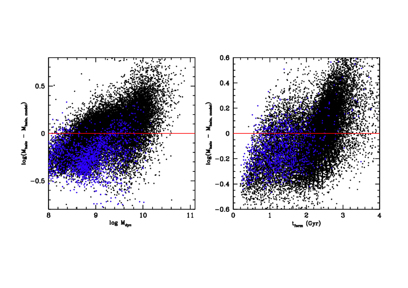

To further demonstrate this, we show that the difference in the halo mass and the best fit model mass based on just the stellar mass (eq. 5) has residuals that correlate with both the dynamical mass and the time-scale of formation (Figure 4). This is such that the scatter in the relationship correlates with each parameter whereby those masses that are overfit (negative values) formed earlier and have lower dynamical masses, and those which are underfit (positive values) have later formation times and higher dynamical masses.


log M log M
Redshift
0.4
0.12
0.58
4.46
2.09
-0.82
-1.57
0.7
0.12
0.56
4.60
2.01
-0.68
-2.02
1.0
0.15
0.51
4.82
1.79
-0.40
-2.52
1.3
0.18
0.47
4.98
1.63
-0.24
-2.51
1.6
0.21
0.43
5.10
1.49
-0.06
-2.88
1.9
0.22
0.41
5.12
1.36
0.10
-3.15
log M log M
Redshift
0.4
0.53
0.04
5.78
1.25
-0.05
-0.68
0.7
0.52
0.04
5.82
1.37
-0.02
-2.08
1.0
0.52
0.05
5.82
1.47
0.02
-3.46
1.3
0.51
0.07
5.82
1.49
0.06
-3.89
1.6
0.51
0.10
5.72
1.51
0.12
-4.35
1.9
0.50
0.16
5.53
1.52
0.16
-4.55
log M log M
Redshift
0.4
0.41
0.07
6.89
1.23
0.09
-1.31
0.7
0.41
0.09
6.89
1.29
0.11
-1.86
1.0
0.41
0.11
6.90
1.35
0.13
-2.40
1.3
0.41
0.14
6.94
1.33
0.16
-2.32
1.6
0.40
0.17
6.98
1.36
0.20
-2.59
1.9
0.39
0.21
7.03
1.38
0.24
-2.91
log M log M
Redshift
0.4
0.32
0.28
5.39
0.11
1.14
-0.97
0.7
0.36
0.25
5.31
0.13
1.22
-2.02
1.0
0.37
0.24
5.33
0.20
1.23
-2.86
1.3
0.38
0.23
5.38
0.33
1.13
-3.09
1.6
0.38
0.23
5.38
0.41
1.10
-3.51
1.9
0.38
0.23
5.36
0.50
1.00
-3.44
IV.3 Halo Masses from Dynamical Masses using Models
IV.3.1 Methods and Results
Our goal in this section is to examine the relation between the observed dynamical mass and halo masses of galaxies at . We furthermore also investigate the use of the S0.5 parameter for measuring the halo masses of galaxies.
One reason for investigating this in detail is that based on the results of §4.2, the scatter in the stellar mass to halo mass relation is reduced by including the dynamical masses, ages and halo concentrations in the inference of halo mass from the stellar mass. It might be the case, and indeed we later continue to show, that the relation between Mdyn and Mhalo has a lower scatter and cleaner correlation than between halo mass and stellar mass.
Based on this we make the assumption that the dynamical mass is a better indicator of the halo mass than the stellar mass, as not only does it have a reduce scatter, but also it is a measure of the internal motions of galaxies, and thus more directly aligned with a measurement of the halo properties than the stellar mass, which is based on complicated baryonic physics and star formation histories (e.g., Hearin & Watson 2013).
We investigate this using both the Galacticus and Millennium simulation results. We find that the two models give essentially the same pattern between the dynamical mass and halo mass. We use the values of the half-mass radius, velocity dispersion and maximum rotational velocity from the Galacticus simulation to determine the relation between Mdyn and Mhalo using the calculation of Mdyn from eq. 2, as well as when we use the Vmax value instead of S0.5.
When we compare the relationship between Mdyn, as measured using S0.5, and the halo mass we obtain Figure 5. The best fitting relation between these parameters is given by:
| (11) |
Where we list the values for and in Table 8. As can be seen, there is very little evolution in redshift in these parameters, and in fact on average the predicted dynamical mass to total mass relation does not change much up to in these models.
We now ask the question of whether it is better to use these dynamical masses or stellar masses to obtain Mhalo. Essentially, we want to derive Mhalo from observations, and it is likely that M∗ or some form of dynamical mass is the best way to do this. For a method of deriving Mhalo to work well we want a maximum sensitivity, i.e, as you move along the ‘observed’ axis, small changes produce a significant amount of change in the halo mass measure. Flat relations like that seen for the sigma mass in §4.3.3 have ’shallow’ fits where similar halo masses are retrieved for a range of ‘kinematic’ masses. However, we also do not want a very steep relationship, such that small changes in observables produce large changes in halo masses. This is because all observables have uncertainties, and inaccuracies are magnified by a very steep relationship.
Ideally, we want something which has a 1:1 slope as much as possible, and this is provided more by the relation between dynamical vs. halo masses than by the stellar vs. halo mass relations. This can be seen by the slopes in the Mdyn vs. Mhalo relations shown in Table 8 which have values of . This way, galaxy halos can be derived with maximum sensitivity, without inducing large errors. Note that this criteria for deriving maximum usability is in concert with minimizing the scatter, which Mdyn vs. Mhalo also does (Figure 3).
Therefore we conclude that using a dynamical mass is superior to using a stellar mass to obtain the halo mass. Using the Moster et al. (2010) formalism (see Appendix) we are also able to retrieve a good fit, particularly for the lower mass galaxies. We hereafter use this as the model method for finding the total halo masses of galaxies based on their dynamical masses as measured from the kinematics and sizes of galaxies.
| Redshift | ||
|---|---|---|
| 0.4 | 1.340.02 | -1.800.26 |
| 0.7 | 1.210.02 | -0.430.23 |
| 1.0 | 1.290.04 | -1.220.40 |
| 1.3 | 1.210.02 | -0.430.23 |
| 1.6 | 1.200.03 | -0.300.26 |
| 1.9 | 1.210.05 | -0.450.45 |
However, it must be noted that in a real sense these ‘measures’ are model dependent, and as such when we compare with other methods of measuring the halo mass we are in a sense testing this methodology for measuring the halo masses of galaxies based on observational features. This methodology is thus not ideal, as it relies on semi-analytical models, and is not based on fundamental observations or derivations. However, if the mass profile of real galaxies is similar to those in the models we use, our methodology should be effective at tracing the halo masses of individual galaxies. Importantly, this method is superior to just using the stellar mass.
This is also not fundamentally different from halo masses measured through abundance matching, or clustering, where there is an assumption about dark matter halo masses and how these are distributed in abundances and clustering. Alternative methods of deriving and their comparisons between the total masses from lensing or the kinematics of large radii tracers such as clustering will be addressed below.
IV.3.2 Comparison to Virial Mass at Virial Radius
Another direct way to measure the total or halo mass of a galaxy is to use, for disk like galaxies, the circular velocities and virial radius to make a measurement of the halo mass. This can be done using theoretical arguments which relate observed quantities of the effective radius to the virial radius, as well as the circular velocity to the Vmax values which are measured directly from the data.
This can be done in the following way, as first outlined in a similar way in Lampichler et al. (2017). The relationship between the effective radius and the virial radius is given by Kravtsov et al. (2013) and Agertz & Kravtsov et al. (2016) using using the abundance matching assumption that such that:
This equation however requires us to know the half-mass radius, as opposed to the half-light or effective radius, which is what we have measured for the bulk of our galaxies. However, when the half-light radius is compared to the half-mass radius, using the mass maps of galaxies, there is little systematic difference found. Therefore we use the value of the effective radius when measuring the virial mass through this method, i.e., (e.g., Lanyon-Foster et al. 2012).
The next step when converting observations to virial masses through this method requires that we use the circular velocity, rather than the maximum velocity. For this we find that the circular velocity to maximum velocity ratio is given by Cattaneo et al. (2014) such that . We compare our masses measured through this approach using the equation:
| (12) |
which we call the circular masses. We compare these masses with those obtained through our direct approach. The result of this is shown at three different redshifts in Figure 6, where there is a good overlap with the mass measurements using our approach. This is particular the case for those systems which are rotationally dominated with , as shown by the blue points in Figure 6. The analytical relation goes through these points expect at the highest masses.
IV.3.3 Sigma Masses - Early Type Galaxies
A popular method for obtaining the total masses of early type galaxies or ellipticals that are dominated by their velocity dispersion is to use the formula:
| (13) |
which we call the sigma () mass. This is often used to determine the total masses of galaxies, even at high redshifts (e.g., Treu et al. 2005). We show in Figure 7 the relationship between the sigma mass and the halo mass found within the Galacticus models. We find that the sigma mass is a good tracer of halo mass at the highest masses, where log M, but note that the highest mass end of this relation is dominated by galaxies with large sizes.
We also plot this ratio between the halo mass and the sigma mass on the right hand panel of Figure 7. This demonstrates that the halo mass of the highest mass elliptical galaxies can be retrieved from the measurement of internal velocity dispersions () for most, but not all of these high- galaxies.
We furthermore find that the relation between the halo mass and the sigma mass is not well fit by a power-law between the two, as we find for the halo mass and the dynamical S0.5 mass. In fact, we find a good fit when we use the formalism between halo and stellar mass found by Moster et al. (2010) derived from abundance match samples. We show this best fit as the red line in Figure 7. We discuss this relation in more detail in the Appendix.
IV.4 Abundance Matching Masses
We further investigate the halo mass to stellar mass ratios from halo abundance matching using stellar masses calculated using the same methodology and underlying techniques as we do for the primary sample’s stellar masses. The basic idea behind this method is to use measured stellar mass number densities at various redshifts and dark matter relation predictions to determine the halo masses for systems with the same abundances (e.g., Kravtsov et al. 2004; Shankar et al. 2006; Conroy et al. 2007; Moster et al. 2013; Behroozi et al. 2013; Shankar et al. 2014; Buchan & Shankar 2016).
Our primary method is to use the number densities for galaxies as a function of redshift as derived by Mortlock et al. (2015), who furthermore use the Chabrier IMF and fitting methods that we use for our measured stellar masses when comparing with kinematic dynamical masses. We then match these number densities, which get higher at lower masses, to that of dark matter halo abundances at the same redshifts and thereby associate each mass range with a halo mass range.
To carry out this comparison, the mass function of dark matter halos (including sub-halos) is assumed to be monotonically related to the observed stellar mass function of galaxies with zero scatter. This relation is given by,
| (14) |
where, and are the number densities of galaxies and dark matter halos, respectively.
To derive these we use the Jenkins et al. (2001) modification to the Sheth & Tormen (1999) halo mass function, the analytic halo model of Seljak (2000), and generate the linear power spectrum using the fitting formulae of Eisenstein & Hu (1998). Based on this the predicted number density of dark matter halos is given by,
| (15) |
Where is the scale independent halo mass function, ( is the value for spherical over-density collapse). is the variance in spheres of matter in the linear power spectrum, is the mean density of the Universe, and is the average number of halos, including sub-halos where we assume the fraction of sub-halos (fsub) is described by,
| (16) |
as in Conroy & Wechsler (2009). Note that this fraction is small and therefore has little effect on our results, but we include it for completeness. Our method basically assigns the most massive galaxies, as measured in stellar mass, to the most massive halos. Given its simplicity it is reasonably successful at matching various observations at multiple epochs (e.g., mass-to-light ratios, clustering measurements, see Conroy & Wechsler 2009 and references therein).
We find that the fits between the stellar mass and halo mass with abundance matching is well represented by the following analytical functions at and as:
| Redshift | |||
|---|---|---|---|
| 0.40 | 3.680.25 | 9.270.28 | 11.22 |
| 0.70 | 2.680.29 | 9.410.28 | 11.22 |
| 1.25 | 2.730.38 | 8.530.16 | 11.22 |
| 1.75 | 8.280.35 | 8.000.05 | 11.22 |
| 2.25 | 2.690.34 | 8.460.05 | 11.22 |
| 2.75 | 3.640.77 | 6.390.08 | 11.22 |
| (17) |
which are all fits with low values. The results of these fits are shown in Table 9. This differs slightly from other parameterizations which include up to five parameters (Behroozi et al. 2013), yet this is the simplest form that fits our data.
We compare the relation between the halo masses derived from abundance matching and the stellar masses at the same limits in Figure 8. The halo masses derived from abundance matching are derived based on the most massive galaxies at each corresponding stellar mass. Thus it is possible, and likely even, that galaxies which are within larger halos are found to higher a higher halo mass at lower stellar mass through abundance matching than what we find through the model masses derived in §4.1.
We show this comparison at redshifts from z = 0.4 to z = 3. First, we note that there is a small amount of evolution in the halo to stellar mass ratio as a function of redshifts, which is also what we find when we investigate this relationship using the observable relations from simulation output (§4.1). Although we note that at the relation is higher, such that the halo mass is larger at a given stellar mass, particularly at lower masses. At higher masses the trend is not as clear.
We also overplot on Figure 8 the relation between halo and stellar mass derived from the model masses derived from stellar mass (eq. 5, §4.1) at redshifts and . There are some differences between the abundance matched based masses and the stellar mass based model masses, particularly at the lower mass range, however this is due to the fact that there is unlikely a 1:1 galaxy:halo ratio at these masses, something we investigate and discuss further below. Hence we get an overestimate of the individual halo masses for these systems using abundance matching. This is not an unexpected result to some degree within this formalism, and this effect has been seen before by e.g., Conroy & Wechsler (2009). We compare the calculated halo masses as a function of stellar mass using the model approach from eq. (5) to those from abundance matching in Figure 9, which shows the ratio of the halo model masses vs. the abundance match masses.
Overall, we find that the average difference between the two methods of measuring Mhalo is less than a factor of three at log M 10.5, which is the primary mass range we study here. This difference is such that the abundance matching masses overestimate halo masses by a factor of roughly 1.5-3 compared to dynamically based halo masses at log M. The halo masses are similar within these two methods at the highest masses. However, at log M the difference is large, a factor of , between the abundance match based masses and those from the models. This is likely due to abundance matching locating these lower mass galaxies in overall higher halos as few systems are isolated.
This shows that our method of measuring the halo masses for massive galaxies through models is roughly consistent with other independent methods at the highest masses, and thus likely to be reliable given that halo abundance matching reveals nearly the same halo masses for a given stellar mass in the range we are interested, with an uncertainty similar to that of measuring the stellar masses. We furthermore compare our results to other abundance matching results, as well as with gravitational lensing ones in §5.
V Observational Results
In this observational results section we first describe the relations between the various masses calculated in §3 and §4 for actual galaxies, including using our new derived individual halo masses. This is followed by a discussion of how these results can be applied towards understanding how galaxy assembly occurs in terms of its major mass components. Later, in the discussion section we discuss the implications of these results.
V.1 Mass Scaling Relations
In this section we use the various measured and calculated stellar, dynamic, and halo masses to link the stellar and dark masses of galaxies up to for our mostly star forming primary sample. This includes investigating how stellar mass relates to these other masses observationally. Ultimately, we are interested in applying these relations to data to infer galaxy evolution, which we discuss in §6..
V.1.1 The Tully-Fisher Relation

For a first step towards investigating evolution of the different dark masses in galaxies, we construct a Tully-Fisher relation (hereafter TFR) for our sample and compare this to the simulation data that we use to convert dynamical into halo masses. Using the primary sample in this paper, Kassin et al. (2007) use the S0.5 parameter to construct a new type of stellar mass Tully-Fisher relation which takes into account the ionized gas velocity dispersion (S0.5/M∗TFR; hereafter kinematic TFR). The form of this Tully-Fisher relation given by:
where is the slope of the relation and is the intercept. This kinematic TFR is considerably tighter than TFRs calculated without taking into account the velocity dispersion, and has no detectable evolution over the redshift range .
We show the S0.5 Tully-Fisher relation in Figure 10 at redshifts and at . As can be seen there is a good relationship between the stellar mass and the values of S0.5 at both high and low redshifts. This involves galaxies of different types. Furthermore, we also plot on these relations the prediction between these two quantities at both high and low redshift from the Galacticus simulation output. As furthermore can be seen, we find a good agreement with the location of our data and theoretical model output, demonstrating that we can use these simulations as a good cosmological representation of all galaxies up to .
V.1.2 Dynamical and Stellar Masses

In this section we compare the dynamical masses in our primary sample from eq. (2) to their corresponding stellar mass measurements. We plot the dynamical masses for the primary sample as a function of stellar mass in Figure 11. We fit the stellar-to-dynamical mass relation for this primary sample as:
| (18) |
From Figure 11 it is clear that the dynamical mass, as we define it, within the visible radius is dominated by the baryonic and stellar mass. As can also been seen in Figure 11, it is clear that this ratio of dynamical to stellar mass does not change significantly at different redshifts up to .
There is an interesting feature in the stellar to dynamical mass plot which deserves a more careful look. This is the fact that the stellar mass for the primary sample, as well as the elliptical sample from Treu et al. (2005) has the interesting property that the stellar mass is higher than the dynamical mass. This is certainly partially due to the way in which we define the dynamical mass and how it gives a better idea of the total mass for elongated and rotating systems than for compact systems such as ellipticals. The reason for this has to do with the fact that the total mass of spheroids is usually calculated with a constant in front of our dynamical mass equation, with most using ‘5’ (see §4.3.3). This is 0.7 dex, which is roughly the amount of the difference seen between the 1:1 ratio and the location of where ellipticals are located, both in the Treu et al. sample in our primary sample.
We furthermore use these relations to derive how the ratio of the stellar mass to dynamical mass changes with both dynamical and stellar mass. We find overall that these relations are indeed quantitatively relatively constant as a function of redshift. Examining the relationship between stellar and dynamical mass we find a best fit of:
| (19) |
and for the relation in terms of stellar mass we find,
| (20) |
Overall this reveals that the stellar mass ratio goes as and . This shows that within the visible extent of galaxies the efficiency of galaxy assembly, defined as having higher M∗ to total mass, is larger at higher dynamical and stellar masses up to our limit of log (Figure 1).
We plot the ratio of stellar mass to dynamical beta mass against redshift in Figure 12 for our primary sample, divided into morphological types, and in Figure 13 for the total sample. We find that the evolution of this ratio with redshift over the entire sample can be fit as:
| (21) |
However, the bulk of this evolution occurs at . If we carry out this fit at , we find a flat slope with (MM. On the other hand we find an increase from to such that (MM.
This essentially means that there is very little to no evolution in the ratio of stellar to dynamical masses at the highest redshifts. A caveat must be put onto this however as our sample at higher redshifts are probably not representative. However we are likely sampling the more gas rich galaxies at these redshifts, and thus we would expect that value to increase, yet it remains statically flat, at least in our overall sample.
As a further way to test this, we investigate the BOSS sample from SDSS III, using galaxies with high masses at M M, typically higher than those considered in this paper. In Figure 14 we show this relationship for galaxies from the BOSS sample at . When we do a least squares fit to this relationship between stellar to sigma mass ratio for galaxies between M M and redshift we find the relationship:
| (22) |
where there is a slight increase with redshift in this ratio for the entire BOSS sample. This implies as well that there is some evidence for evolution in this ratio at , within the highest mass galaxies. We later investigate this relationship for higher redshift systems in §5.2 using the total halo masses of our systems.
Furthermore Figure 12 is also plotted by morphological type as measured by the CAS parameters (§2.2). Based on this, we find that the early-type systems have a slightly higher stellar-to-dynamical mass ratio than other morphological types at all redshifts. This is potentially a sign that the efficiency of galaxy formation is higher in early-type galaxies than disks/late-types/mergers. This is not a trend which results from the early type galaxies being more massive, as in our primary sample the ellipticals are not more massive on average than the other morphological types (Figure 1). This shows observationally that there is a third parameter in the relation of dynamical mass to halo mass, consistent with age as a third parameter as discussed in §4.2. This must be related to the galaxy morphology and time of formation which correlates with the concentration of the halo/galaxy. We investigate this in more detail in §6.
V.1.3 Halo Mass vs. Stellar Masses
We now use these results to examine the relation between the halo and the stellar mass for our sample of real galaxies. We show in Figure 15 the halo masses derived from §4 as a function of stellar mass for our entire observational sample. The dashed black curved line shows the best three component theory fit from eq. (5), showing a reasonably good agreement with the data at the highest masses. We attempt to improve the above fit and minimize scatter by investigating the stellar-to-halo mass fit when galaxies are binned by morphology and stellar mass density. There is a slight improvement in these fits when the sample is binned by morphological type or by stellar mass surface density.
Figure 16 shows the stellar mass to halo mass ratio as a function of stellar mass for our entire sample using both primary and secondary sources. To compare our halo masses with that of other work, we plot our results with those of Foucaud et al. (2010), van Uitert et al (2016), Leauthaud et al. (2012), and Moster et al. (2013). These studies use different techniques to measure the halo masses of galaxies as described in §2.4. The observational studies are shown as points of various shapes and colours.
In the mass range M∗/M we broadly agree with previous results, except for the Treu et al. (2005) ellipticals. There is also an interesting feature in these figures such that there is no obvious turn-over in the M∗/Mhalo ratio which reaches a maximum at about log M. This turnover is seen in other samples at this halo mass based on clustering (e.g., Foucaud et al. 2010; Coupon et al. 2012). For example, the peak found by Coupon et al. (2012) it is log Mhalo = 11.6 from clustering and in Coupon et al. (2015) is log M. We are able to probe down to log M, yet we do not see an obvious turnover in the ratio of stellar to halo mass to this limit.
This shows that the efficiency of galaxy formation is highest at the highest masses. This relationship is also seen when ones compares the mass ratios by using halo masses as determined from abundance matching (e.g., Behroozi et al. 2013). Figure 17 furthermore shows the ratio of our abundance matching stellar vs. halo masses as a function of stellar mass. This demonstrates that the maximum galaxy formation efficiency is at around log M. Finally, Figure 18 shows the evolution of the ratio of stellar to halo mass as a function of redshift, demonstrating little change with time, as discussed in the follow section.
V.2 Mass Ratios as a Function of Redshift
One of the issues we investigate is how the ratio of stellar to halo mass varies with redshift. This is however a difficult topic to study observationally and our attempts at answering this question should be seen as a preliminary solution until more kinematic and mass data is available for complete samples of galaxies at . However, we can get some idea of this from limited observations of kinematics at various redshifts, as well as through our abundance matched masses.
Overall, however, as we have kinematic data up to we can determine the evolution of this relation up to these redshifts, although for a potentially biased sample of mostly star forming galaxies (§2.3). Figures 12 & 13 plot stellar-to-dynamical mass ratio as a function of redshift up to for our primary and total sample, while Figure 19 plots the M∗/Mhalo ratio against redshift for all of the observational samples compared with theory predictions and other observational results. For all samples of galaxies up to we find a best fitting relationship of the form:
| (23) |
This is consistent, within 1, of this ratio being flat, i.e., does not evolve with redshift. We do find an evolution with a significant slope for the sample at with , as we do for the ratio of the dynamical to stellar mass.
This shows that the majority of the evolution in terms of stellar vs. halo mass occurs at later times when galaxies are primarily finished with their star formation, and are evolving more in terms of galaxy mergers (e.g., Mundy et al. 2017). In summary, we find no significant evidence for any change in the M∗/Mdyn ratio at the highest redshift, although we do find an evolving ratio at lower redshifts, .
We also find very little evolution in the stellar to halo mass ratio when using the abundance matching technique (§4.4). We show in Figure 18 the evolution of the ratio of stellar to halo mass as derived from the abundance matching methodology. Overall, we find that the stellar mass ratio does not significantly evolve with time at any measured stellar mass as measured either from the kinematic based model halo masses, or from using abundance matching.
We fit the evolution of these mass ratios from abundance matching in the form of
The values of the best fitting parameters are and for galaxies with log , , for log systems, , for log , , for log and , for log . With the only case which has a significant slope of is for the highest masses with log .
Our results are in agreement with Conselice et al. (2005), who also find that the highest mass galaxies have the highest M∗/Mhalo ratio. Furthermore, using galaxy clustering, Foucaud et al. (2010) find a declining M∗/Mhalo ratio with redshift at , at a given stellar mass selection. However, Foucaud et al. (2010) effectively measure the parent halo of objects while we are observing the halo mass for individual ‘sub-halos’. Foucaud et al. (2010) interpreted this evolution as a halo downsizing effect.
However, we must keep in mind that the kinematic model mass evolution in the mass ratios is biased. The galaxies towards the higher redshifts are more typically star forming galaxies, with a later-type morphology, and there is no guarantee that these systems are representative of the population as a whole at these redshifts. Our results at should therefore be taken with caution as a preliminary measure of how total and stellar masses relate at higher redshifts.
VI Discussion
VI.1 Dark Matter Accretion Rates
These results have implications for the way in which galaxy formation occurs at . With the observation of a nearly constant stellar to total mass ratio with redshift we can derive the accretion rate of both gas, as well as dark matter, building the halos and galaxies over cosmic time. We start off with a method for parameterizing the star formation history, which for our sample can be represented by an exponentially declining star formation, such that the star formation rate as a given redshift can be written as

| (24) |
where is the initial star formation rate; is the elapsed time since the star formation rate began, and is the characteristic declining rate of the exponential. This form is a good fit to the stellar populations of galaxies at (e.g. Mortlock et al. 2013; Ownsworth et al. 2014). Integrating this between two times, and , we obtain a measure of the amount of stellar mass created between these two epochs:
| (25) |
if we take the star formation rate to begin at then this equation reduces to
| (26) |
In what follows we consider as well the amount of stellar mass which is returned to the ISM of these galaxies after taking into account the results of stellar evolution after 1 Gyr (e.g., Conselice et al. 2013; Ownsworth et al. 2014). If we furthermore consider the form of the ratio of stellar mass to total mass, i.e.,
| (27) |
then a change in stellar mass corresponds to a change in the total mass given by
| (28) |
Where we have used the observation that is roughly independent of redshift at . Using this, we can then consider how the star formation rate relates to the change in the stellar mass as given by eq. (26) over a large time period. Between and the addition of total mass to the system can be calculated by combining with eq. (28). We can then write,
| (29) |
however, we can also consider the instantaneous rate of accretion of material in terms of a star formation rate if we use the approximation that . Using this we can then write the mass accretion rate as
| (30) |
where is the equivalent star formation rate after accounting for the amount of mass returned to the ISM through stellar evolution processes. Effectively, this is the stellar mass formation rate, rather than just the star formation rate. Through the use of stellar evolution models the effective stellar mass formation rate is around 70% of the star formation rate after a few Gyr.
From Ownsworth et al. (2014) we know how the star formation rate of galaxies with similar masses to those studied here evolves. Overall, the star formation rate is given by the form in eq. (24), with Myear-1 and years. Furthermore, the observed star formation rates are: Myear-1 at ; Myear-1 at ; and Myear-1 at .
Using the value of given in Section 5, and using eq. (30) we calculate the total mass accretion rate. We show these calculated values as a function of mass and redshift in Figure 20. This figure reveals that the total mass accretion rate for typical galaxies varies with stellar mass and redshift. We find that the peak halo accretion rate is around: Myear-1 at . This is much higher than the stellar mass or the gas accretion rates at similar redshifts (e.g., Conselice et al. 2013; Mortlock et al. 2014; Ownsworth et al. 2014).
We find that within our assumptions galaxies grow their total integrated halo mass Mhalo at a self-similar rate as their stellar M∗ masses. The M∗ growth can be explained by the process of mergers (both major and minor) triggering star-formation events which increases M∗. The gas for this must come from both minor/major mergers, as well as gas accretion (e.g., Conselice et al. 2013; Mundy et al. 2017). The fact that the dark matter accretion rate follows that of the star formation rate, revealing a nearly constant ratio at , implies that the dark matter is being accreted with the baryons in these galaxies to build up the mass of the system at this epoch.
We can also compare these values to theory which predicts, even based on analytical calculations, what the accretion rate of dark matter is onto halos (e.g., van den Bosch et al. 2002; Wechsler et al. 2002; McBride et al. 2009; Correa et al. 2014). For example, Wechsler et al. (2002) predict an accretion history which scales as an exponential: Me-αz.
It is proposed based on these various simulations and calculations using the Extended Press-Schechter (EPS) formalism that the total mass accretion history can be represented by a combination of an exponential and a power-law in the form (e.g., McBride et al. 2009; Correa et al. 2014):
| (31) |
Taking the derivative of this, we find that the rate of change of the halo mass is given by (e.g., Correa et al. 2014)
where is the halo mass of the galaxy in units of M, and and are the cosmology.
When we fit our data and observations to this we find that the values of and are as given in Table 10. This is in agreement with our observations, as can be seen in the comparison in Figure 20. This is similar to the results of the mass accretion rates derived from other, but similar, assumptions (e.g., e.g., Behroozi et al. 2013; Rodriguez-Puebla et al. 2017).
| Density (Mpc-3) | log M∗ | log Mhalo | ||
|---|---|---|---|---|
| 5 | 10.8 | 12.4 | -0.441.25 | -0.880.41 |
| 1 | 11.2 | 13.1 | -0.120.37 | -0.200.11 |
| 4 | 11.4 | 13.3 | 0.070.33 | 0.210.11 |
VI.2 Dark Matter Mass as a Regulator of Galaxy Formation
One of the goals in this paper is to relate the matter components of galaxies beyond the local universe, and to develop a method for doing this which can be applied to single galaxies, as opposed to stacked systems as used in clustering and lensing (e.g., Coupon et al. 2015). In general we find that the stellar mass is, within some scatter, a good tracer of the dynamical mass and halo masses of field galaxies at within our mass range. This may not be the case for red passive galaxies, or for those in very dense areas such as clusters, which are not present in our sample in great abundance.
This suggests that the different masses in galaxies, and how they build up over time, are highly regulated by the overall halo mass of the galaxy which drives the formation of the amount of stellar mass within these galaxies. That is, fundamentally the formation of galaxies is hierarchical with dark matter accreted from the IGM the main way mass is built up. When this dark matter is accreted baryonic mass is as well, which leads to additional galaxy formation processes such as star formation and likely AGN activity. This also suggests that galaxies are assembling hierarchically, independent of the method in which mass is brought into the systems, whether it be through mergers of various types or through e.g., gas accretion processes.
This is similar to previous findings from other papers, including Kravtsov et al. (2014) where the masses of brightest cluster galaxies (BCGs) have a stellar mass which scales with total mass (M500) such that M M with a scatter in M500 of 0.2 dex for centrals. Satellite galaxies within this sample have s scaling which goes as M M with a smaller scatter of 0.1 dex. This is similar to our results when we examine the scaling between the stellar mass and halo mass for our systems (§5.1.2).
VI.3 Galaxy Formation Efficiency
A standard way to characterize the efficiency of galaxy formation is to compare the stellar masses of galaxies to their halo masses, and to find where this ratio peaks as a function of stellar mass and redshift. Furthermore it is interesting to determine if this peak changes as a function of redshift, as well as if different methods give different answers to this observational question.
It is well known that the peak of the galaxy formation efficiency, i.e., when the stellar to dark matter masses peaks, is at roughly log or log M (e.g., Behroozi et al. 2013) through the use of abundance matching. Our results show a few things that are worth discussing in detail and following up, as we do not find such clear cut evidence for a turn over, at least to within the mass limits of our sample.
First, we find that the ratio of stellar mass to halo mass declines as we observe galaxies at lower stellar masses at . This is as expected, and shows that the galaxy formation process efficiency is lower for lower mass galaxies, as seen in the comparison points from abundance matching and lensing as shown in Figure 16. However, we do not find a ‘peak’ in the galaxy formation process, as we find a continual increase in the ratio of stellar to halo mass for individual galaxies as we go to higher masses. This suggests that the dark matter masses we are measuring are only for single galaxies, and not large halo masses as what might be measured in groups or clusters of galaxies. Our samples are generally not taken from dense environments, and this may be one reason we do not see an enlarged halo mass for the highest mass galaxies.
There is also the issue that the peak in the galaxy formation may evolve with redshift, as is found in halo clustering derived masses (e.g., Coupon et al. 2012). However, this is likely due to the fact that the halo masses derived with clustering measures are observing more the massive parent halo masses due to halo downsizing. We do not see any evidence for an evolution in the ratio of stellar to halo mass, nor do we see evidence that the galaxy formation efficiency peak is changing at higher redshifts.
Based on current ideas, we would expect the stellar mass to halo mass ratios for the most massive galaxies to decline from a peak at the highest masses. We would see this as the most massive galaxies having the largest relative dark matter content. This is usually interpreted as being due to AGN feedback which is most effective at the highest stellar and halo masses which prevents gas from cooling to form stars. The fact that we do not see this, at least when we compare this ratio with stellar mass, suggests that halo masses for these very massive galaxies we are measuring are for the halo associated with just the galaxy itself, and not the overall larger halo that might be present. This may alternatively imply that the effects of AGN feedback are not important for determining the total amount of baryonic mass formed, or that the effects are most pronounced in the outer parts of halos.
In fact, the greatest effect we see is a form of halo downsizing, whereby the earliest galaxies to form in the ‘oldest’ halos have the largest stellar mass to dark matter mass. This implies that the time these halos forms is more critical for their overall ‘efficiency’ of galaxy formation than any other process. We can see this with a higher stellar mass to halo mass ratio at a given mass for systems which are ellipticals compared with for example disks. This higher stellar to halo mass ratio is also seen in the models, suggesting that the time of formation is indeed the third parameter in the correlation between the stellar mass and halo masses of galaxies which correlates with the dynamical mass (§4.3).
VII Conclusions & Summary
In this paper we examine the different forms of galaxy mass (stellar, dynamical, halo) at high redshifts from . We take as our starting point a well defined sample of 544 galaxies with well measured star formation rates, kinematics and sizes and derive relations between the derived gas masses, dynamical masses and halo masses. We find the following major results.
1. Galaxy halo and dynamical masses can be successfully retrieved used the S0.5 index which combines the use of a galaxy’s velocity dispersion and its rotational velocity. This is superior to using just a velocity dispersion or a rotational velocity and allows the measurement of halo masses on individual systems as opposed to ensemble averages. We furthermore argue that the third parameter in this fit is the time of halo formation with systems forming earlier having a higher stellar to halo mass ratio.
1. There is a strong relation between the stellar mass and dynamical masses for galaxies that occupy their own massive halos (i.e., field galaxies). This suggests that galaxy formation is highly regulated and the different masses are correlated and assemble together in galaxies.
2. We show that within the visible radius, dynamical masses of the galaxies in our sample are dominated by stellar mass up to .
3. We derive the halo masses of galaxies by using semi-analytical models which show how to relate the velocity of rotation, size and halo mass together. This method shows that the most massive galaxies in stars have the highest ratios of stellar to halo mass, while the least massive galaxies have the lowest ratios.
4. We develop a series of empirically based relations between the stellar mass of galaxies and their dark masses as a function of redshift. The scatter in these relations are just slightly higher than the expected error budget in stellar masses, with a dispersion of around dex.
5. We use the fact that the stellar to halo mass does not appear to change significantly with redshift at to argue that the dark matter accretion rate is Myear-1 at down to a accretion rate of a few hundred Myear-1 by .
In the future, these types of observations can be extended with longer exposures obtaining deeper kinematic data in the outer parts of galaxies which will hopefully give us a better and more accurate idea of the halo masses for these systems. Doing this is however very difficult with current technology, and may require the use of spectrographs on 20-30m telescopes in the next decade. In the mean-time clustering and lensing analyses of masses will make headway in terms of average galaxy properties and we can measure mass evolution for bulk galaxies divided into finer subsets.
ACKNOWLEDGMENTS
We thank the referee for their comments which significantly improved the presentation of this paper. We thank Alice Mortlock, Jamie Ownsworth and Seb Foucaud for their comments and help with various aspects of this paper, and Andrew Benson for help with the use of the Galacticus models. We thank Sedona Price and the rest of the MOSDEF team for making their data available, and to Alessandra Beifiori for making her SDSS-III galaxy internal measurements of sizes and velocities available. We acknowledge support from the Leverhulme Trust in the form of a Leverhulme Prize to CJC and funding from the STFC as well as financial support from the University of Nottingham.
References
- [1] Agertz, O. & Kravtsov, A.V. 2016, ApJ, 824, 79
- [2] Bauer, A. E., Conselice, C. J., Pérez-González, P. G., et al. 2011, MNRAS, 417, 289
- [3] Behroozi, P.S., Wechsler, R.H., Conroy, C. 2013, ApJ, 770, 57
- [4] Beifiori, A., et al. 2014, ApJ, 789, 92
- [5] Bell, E. F., McIntosh, D.H., Katz, N., Weinberg, M.D. 2003, ApJS, 149, 289
- [6] Berlind, A.A., et al. 2003, ApJ, 593, 1
- [7] Binney, J., & Tremaine, S. 1987, Princeton, NJ, Princeton University Press, 1987, 747 p.,
- [8] Bonnet H., Abuter R., Baker A. et al., 2004, The Messenger, 117, 17
- [9] Bruzual G., Charlot S., 2003, MNRAS, 344, 1000
- [10] Buchan, S., Shankar, F. 2016, MNRAS, 462, 2001
- [11] Bundy K., Ellis R. S., Conselice C. J. et al., 2006, ApJ, 651, 120
- [12] Cappellari et al., 2006, MNRAS, 366, 1126
- [13] Cappellari et al., 2013, MNRAS, 432, 1709
- [14] Chabrier G., 2003, PASP, 115, 763
- [15] Cole S., Lacey C. G., Baugh C. M., Frenk C. S., 2000, MNRAS, 319, 168
- [16] Conroy, C., Wechsler, R.H. 2009, ApJ, 696, 620
- [17] Conselice C. J., 2003, ApJS, 147, 1
- [18] Conselice C. J., Bershady, M., Dickinson, M., Papovich, C. 2003, AJ, 126, 1183
- [19] Conselice C. J., Bundy K., Ellis R. S., Brichmann J., Vogt N. P., Phillips A. C., 2005, ApJ, 628, 160
- [20] Conselice C. J., Bundy K., Trujillo I. et al., 2007, MNRAS, 381, 962
- [21] Conselice C. J., Bundy K., Vivian U., Eisenhardt P., Lotz J., Newman J., 2008a, MNRAS, 383, 1366
- [22] Conselice C. J., Rajgor S., Myers R., 2008b, MNRAS, 386, 909
- [23] Conselice C. J., Bluck A. F. L., Buitrago F. et al., 2011, MNRAS, 413, 80
- [24] Correa, C.A., Wyithe, J.S.B., Schaye, J., Duffy, A.R. 2014, MNRAS, arXiv:1409.5228
- [25] Coupon, J., et al. 2012, A&A, 542, 5
- [26] Daddi, E., et al. 2010, ApJ, 714, 118L
- [27] Davis M., Efstathiou G., Frenk C. S., White S. D. M., 1985, ApJ, 292, 371
- [28] Davis M., Faber S. M., Newman J. et al., 2003, Proc. SPIE, 4834, 161
- [29] Davis M., Guhathakurta P., Konidaris N. P. et al., 2007, ApJ, 660, L1
- [30] De Lucia G., Blaizot J., 2007, MNRAS, 375, 2
- [31] Drory N., Salvato M., Gabasch A., Bender R., Hopp U., Feulner G., Pannella M., 2005, ApJL, 619, L131
- [32] Erb, D.K., Steidel, C.C., Shapely, A.E., Pettini, M., Reddy, N.A., Adelberger, K.L. 2006, ApJ, 646, 107
- [33] Eisenhauer F., Abuter R., Bickert K. et al., 2003, SPIE 4841, 1548
- [34] Elsner F., Feulner G., Hopp U., 2008, A&A, 477, 503
- [35] Epinat B., Contini T., Le Fèvre O. et al., 2009, A&A, 504, 789
- [36] Faber, S.M., Gallagher, J.S. 1979, ARA&A, 17, 135
- [37] Flores H., Hammer F., Puech M., Amram P., Balkowski C., 2006, A&A, 455, 107
- [38] Foucaud S., Conselice C. J., Hartley W. G., Lane K. P., Bamford S. P., Almaini O., Bundy K., 2010, MNRAS, 406, 147
- [39] Fontana A., Pozzetti L., Donnarumma I. et al., 2004, A&A, 424, 23
- [40] Förster Schreiber N. M., Genzel R., Lehnert M. D. et al., 2006, ApJ, 645, 1062
- [41] Giavalisco M., Lee K.-S., Ferguson H. C. et al., 2004, AAS, 36, 1497
- [42] Glazebrook K., Abraham R. G., McCarthy P. J., et al., 2004, Nature, 430, 181
- [43] Guerou, A., et al. 2017, A&A, 608
- [44] Hearin, A.P., Watson, D.F., Becker, M.R., Reyes, R., Berlind, A.A., Zentner, A.R. 2014, MNRAS, 444, 729
- [45] Heavens A. F., Panter B., Jimenez R., Dunlop J., 2004, Nature, 428, 625
- [46] Hook I., Jørgensen I., Allington-Smith J. R. et al., 2004, PASP, 116, 425-440
- [47] Hopkins A. M., 2004, ApJ, 615, 209
- [48] Ilbert, O., et al. 2013, A&A, 556, 55
- [49] Kajisawa M. et al., 2009, ApJ, 702, 1393
- [50] Kassin S. A., Weiner B. J., Faber S. M., 2007, ApJ, 660, L35
- [51] Kennicutt R. C., 1998, ApJ, 498, 541
- [52] Kent, S.M. 1987, AJ, 93, 816
- [53] Kobulnicky, H.A., Gebhardt, K. 2000, AJ, 119, 1608
- [54] Komatsu E. et al., 2009, ApJS, 180, 330
- [55] Kravtsov, A.V., Berlind, A.A., Wechsler, R.H., Klypin, A.A., Gottlober, S., Allgood, B, Primack, J.R. 2004, ApJ, 609, 35
- [56] Kravtsov, A.V.,Vikhlinin, A., Meshscheryakov, A. 2014, arXiv:1401.7329
- [57] Kriek, M., Shapley, A. E., Reddy, N. A., et al. 2015, ApJS, 218, 15
- [58] Leauthaud, A., et al. 2012,
- [59] Lampichler, N., Maier, C., Ziegler, B. 2017, arXiv:1707.09838)
- [60] Lanyon-Foster, N.M., Conselice, C.J., Merrifield, M. 2012, MNRAS, 424, 1852
- [61] Mandelbaum R. Seljak U., Kauffmann G., Hirata C. M., Brinkmann J., 2006, MNRAS, 368, 715
- [62] Mannucci, F. et al. 2009, MNRAS, 398, 1915
- [63] McBride, J., Fakhouri, O., Ma, C.-P. 2009, MNRAS, 398, 1858
- [64] McCracken, H., et al. 2015, MNRAS, 449, 901
- [65] McGaugh S. S., 2005, ApJ, 632, 859
- [66] Mendes de Oliveira C., Amram P., Plana H., Balkowski C., 2003, AJ, 126, 2635
- [67] Miller, S.H., Ellis, R.S., Newman, A.B., Benson, A. 2014, ApJ, 782, 115
- [68] Miller, S.H., Bundy, K., Sullivan, M., Ellis, R.S., Treu, T. 2011, ApJ, 741, 115
- [69] More, S., Kravtsov, A., Dalal, N., Gottlober, S. 2011, ApJS, 195, 4
- [70] Mortlock A., Conselice C. J., Bluck A. F. L., Bauer A. E., Grützbauch R., Buitrago F., Ownsworth J., 2011, MNRAS, 413, 2845
- [71] Mortlock A., et al. 2013, MNRAS, 433, 1185
- [72] Moster, B., Naab, T., White, S.D.M. 2013, MNRAS, 428, 3121
- [73] Muzzin, A., et al. 2013, ApJ, 777, 18
- [74] Navarro J. F., Frenk C. S., White S. D. M., 1996, ApJ, 462, 563
- [75] Noeske K. G., Faber S. M., Weiner B. J. et al., 2007, ApJ, 660, L47
- [76] Östlin G., Amram P., Bergvall N. et al., 2001, A&A, 374, 800
- [77] Ownsworth, J.R., Conselice, C.J., Mortlock, A., Hartley, W.G., Almaini, O., Duncan, K, Mundy, C.J. 2014, MNRAS, 445, 2198
- [78] Panter B., Jimenez R., Heavens A. F., Charlot S., 2007, 378, 1550
- [79] Papovich C., Moustakas L. A., Dickinson M. et al., 2006, ApJ, 668, 48
- [80] Pasquini L., Avila G., Blecha A. et al., 2002, The Messenger, 110, 1
- [81] Pérez-González P. G., Rieke G. H., Villar V. et al., 2008, ApJ, 675, 234
- [82] Persic M., Salucci P., Stel F., 1996, MNRAS, 281, 27
- [83] Planck Collaboration, 2014, arXiv:1303.5076
- [84] Price, S., et al. 2016, ApJ, 819, 80
- [85] Rodríguez-Puebla A., Avila-Reese V., Yang X., Foucaud S., Drory N., Jing Y.P. 2015, ApJ, 799, 130
- [86] Rodríguez-Puebla, A., Primack, J. R., Avila-Reese, V., & Faber, S. M. 2017, MNRAS, 470, 651
- [87] Schiminovich D., Wyder T. K., Martin D. C. et al., 2007, ApJS, 173, 315
- [88] Scoville, N. 2016, ApJ, 820, 83
- [89] Shankar, F., Lapi, A., Salucci, P., De Zotti, G., Danese, L. 2006, ApJ, 643, 14
- [90] Shankar, F., et al. ApJ, 797, 27L
- [91] Skibba, R., et al. 2015, ApJ, 807, 152
- [92] Springel V. et al., 2005, Nat, 435, 629
- [93] Ubler, H., et al. 2017, ApJ, 842, 121
- [94] van den Bosch, F.C. 2002, MNRAS, 331, 98
- [95] van Uitert, E. et al. 2016, MNRAS, 459, 3251
- [96] Watson, D.F., Hearin, A.P., Berlind, A.A., Becker, M.R., Behroozi, P.S., Skibba, R.A., Reyes, R., Zentner, A.R., van den Bosch, F.C. 2015, MNRAS, 446, 651
- [97] Weiner B. J., Willmer C. N. A., Faber S. M. et al., 2006, 653, 1027
- [98] Wechsler R.H., Bullock J.S., Primack J.R., Kravtsov A.V., Dekel A. 2002, ApJ, 568, 52
- [99] Weinmann S. M., van den Bosch F. C., Jing Y. P., 2005, MNRAS, 357, 608
- [100] White S. D. M., Rees M., 1978, MNRAS, 183, 341
Appendix A The Meaning and Usefulness of the S0.5 Parameter
As mentioned in the body of the paper, we use the S0.5 parameter (§3.2) throughout to derive the dynamical masses of galaxies, and furthermore we use this measurements as a proxy and as a way to obtain the halo masses of a galaxy. We investigate in this appendix the nature of the S0.5 parameter and how to interpret the resulting dynamical mass calculated from it.
First, we determine how the distribution of S0.5 values in the models match the data. To do this, we compare at both and the distribution of half-light radii and S0.5 values. As shown in Figure A.1 there is a good overlap in these values, i.e., that the simulation we use to calculate the dynamical masses has a good overlap with the actual data at both high and low redshift. This is also the case when comparing with the observed and predicted relation between S0.5 and stellar mass (Figure 10; §5.1.1) in a Tully-Fisher like relation.
The one exception to this is that we observationally do not see high velocity systems which have very small radii in the same abundance as the simulations. We do however find that there are galaxies with larger radii, namely the early-types, which have large S0.5 parameters but which are not abundant in the model itself. We therefore exclude these simulated galaxies in our further analyses which have sizes kpc. We also find systems which have a very small radii and a large value of combined velocities through the S0.5 parameter which we also exclude from our analyses.

The nature of dynamical masses from S0.5 is such that it should represent a good indicator for the total mass within the galaxy itself, or that it correlates in some way with the total amount of mass within the galaxy. Thus, within the brighter portion of a galaxy, within Re, we would expect that the total mass of our galaxies are dominated by the stellar mass, as dark matter would have very little expected contribution to the inner portions of galaxies.
To demonstrate how well this assumption is we plot at three different redshifts the relationship between the dynamical mass and the stellar mass in Figure A2. Here the dynamical mass is measured at exactly the half-light radius, and thus we do not implement the term from eq. 3 here.

As can be seen, there is a good relationship between the stellar mass and the dynamical mass within the Galacticus models. This relationship is nearly 1:1 up to about stellar masses of M Mwhen the relationship becomes softer, particularly at higher dynamical masses at a lower redshifts. However, this difference is less striking at higher redshifts, , where the relationship between these two quantities is slightly improved. This figure however does justify the use of our dynamical mass as a measure of ’mass’ in a galaxy. Given that it is kinematically based, and measured within the visible portions of galaxies, we find that it statically matches the stellar mass at the location where the stellar mass dominates the total mass of a galaxy.
Appendix B Other Fitting Forms
B.1 Modeled Stellar Mass to Halo Mass Relation
There are a myriad of ways that the relation between the stellar mass or dynamical mass can be fit as a function of the halo mass. In this section we discuss some of these fits and give their forms. We also consider how other masses, the circular mass and the sigma mass, are related to the halo mass. First, we consider however alternative methods for measuring the halo mass based on the dynamical mass.
The first relationship we consider is whereby the relation between stellar to halo mass is fit by two power-laws with a break at M Mwhich is the representative location where the slope of the relationship changes. We fit this relation between stellar and halo mass with a linear relationship between the log of these quantities using the form:
| (B1) |
where the quantities for and are listed in Table B1 at the separation point log M. As we find in the main paper we find that there is no evolution in the relationship between stellar and halo masses, at least in these models.
| log M | log M | |||
|---|---|---|---|---|
| Redshift | ||||
| 0.4 | 0.440.04 | 6.80.3 | 1.680.12 | -5.81.3 |
| 0.7 | 0.380.05 | 7.50.4 | 1.650.05 | -5.50.6 |
| 1.0 | 0.400.05 | 7.20.4 | 1.650.04 | -5.40.5 |
| 1.3 | 0.440.05 | 6.90.5 | 1.580.02 | -4.70.2 |
| 1.6 | 0.440.05 | 6.90.4 | 1.550.02 | -4.20.1 |
| 1.9 | 0.420.04 | 7.10.4 | 1.530.04 | -4.00.4 |
We also examine results from the Millennium simulation to see if there is any differences between different models for the relationship between stellar and halo mass. To carry out this comparison we select galaxies from the De Lucia & Blaizot (2007) catalogue at giving us 684,357 galaxies selecting both stellar and halo masses. We use the friend-of-friend halo masses from this simulation as a measure of our halo mass. These friends-of-friends masses are not based on a certain mass threshold, but on a linking length parameter, and there is a variation in the mass overdensity depending upon the concentration of the various mass profiles (e.g., More et al. 2011). The corresponding relationship for the Millennium simulation over our redshifts of interest is given by:
| (B2) |
Where we find a very similar relationship that we find in the Galacticus simulations, which we discuss in the main body of the paper.
B.2 Alternative Dynamical Mass-Halo Mass Relations
B.2.1 Moster et al. (2010) Functional Form
One of the functional forms in which we fit the dynamical to halo mass is through that established by Moster et al. (2010) for the relationship between the stellar mass and the halo mass through abundance matching. The form of this fitting for our relation between the dynamical and halo mass is:
| (B3) |
As discussed in §4.3 the best fitting relations for the Moster et al. (2010) relations is shown as the green line in Figure 5. As also discussed, these fits are not superior to the simplified form of a single power-law relationship between the value of log Mdyn and log Mhalo. We also use this form of fit when fitting the sigma mass to the halo mass in §4.3.3 and Figure 7. It’s likely that this more complex form is more accurate for fitting functional forms, something which can be explored in more detail once models predicting the quantities we study are better calibrated.