Modeling continuous levels of resistance to multidrug therapy in cancer
Abstract
Multidrug resistance consists of a series of genetic and epigenetic alternations that involve multifactorial and complex processes, which are a challenge to successful cancer treatments. Accompanied by advances in biotechnology and high-dimensional data analysis techniques that are bringing in new opportunities in modeling biological systems with continuous phenotypic structured models, we study a cancer cell population model that considers a multi-dimensional continuous resistance trait to multiple drugs to investigate multidrug resistance. We compare our continuous resistance trait model with classical models that assume a discrete resistance state and classify the cases when the continuum and discrete models yield different dynamical patterns in the emerging heterogeneity in response to drugs. We also compute the maximal fitness resistance trait for various continuum models and study the effect of epimutations. Finally, we demonstrate how our approach can be used to study tumor growth regarding the turnover rate and the proliferating fraction, and show that a continuous resistance level may result in a different dynamics when compared with the predictions of other discrete models.
Keywords:
Multidrug resistance, Tumor growth, Phenotype structured model, Epimutation1 Introduction
The biological mechanisms responsible for the emergence of drug resistance and its propagation often involve a multifactorial and complex process of genetic and epigenetic alternations [1, 2, 3], that arise through a series of genetic and non-genetic changes [4, 5, 6, 7]. Such changes can be due to drug administration (drug induced resistance) [8, 9], or they can emerge independent of therapy due to intrinsic mechanisms. Cancer cells may develop simultaneous resistance to structurally and mechanistically unrelated drugs, leading to multidrug resistance (MDR) [1, 2, 10]. The complex dynamical nature of MDR is one of the most challenging obstacles to successful treatment.
The complexity of the mechanisms underlying drug resistance has encouraged its study through mathematical modeling. Such models aim at providing quantitative tools for testing therapies that circumvent or at least delay the unfortunate consequences of drug resistance. Examples include the models of Goldie and Coldman [11, 12, 13] that are based on resistance due to point mutations. These works were proceeded by many studies considering stochastic models (including branching process and multiple mutations) to study MDR and optimal control of drug scheduling [14, 15, 16, 17]. Alternative approach includes continuum deterministic models using ordinary differential equations, for example, modeling kinetic resistance [18] and point mutations [19], and partial differential equations, where spatial heterogeneity and vascularization can be readily incorporated [20, 21, 22]. For additional approaches see [23, 17, 24, 25, 26, 27, 28].
In addition to the aforementioned modeling approaches, the advance of biotechnology in collecting data characterizing the phenotype is bringing in new opportunities of mathematical modeling of biological systems. The most recent technology allows cytometry data to be collected up to O dimensions, Methylation profiles in the scale of O(1000), and gene-expression profile in the scale of O(10000) [29, 30, 31, 32, 33, 34]. In particular, recent advances in single cell RNA sequencing technologies has enabled a new high-dimensional definition of cell states, that is on the order of 20,000 protein encoding genes that compose the transcriptome [35, 32]. The high-dimensionality of the data makes it practically impossible to consider a meaningful model on the original space in which the data is collected. Thus, various dimension reduction techniques, such as, principal component analysis [36, 37], t-distributed stochastic neighbor embedding [38, 30, 39], diffusion maps [40, 41], and machine learning techniques [42, 43], have been employed to reduce the dimensionality and to identify only the critical directions. In contrast to classical biology and modeling approaches, where cell types are classified into discrete states and differentiation is considered as a stepwise process of binary branching decision, the new technologies and data analysis enabled considering cell differentiation as a continuous process that can be mapped into a continuum of cellular and molecular phenotypes [31, 40, 33]. In other words, the high-dimensional configuration space is mapped into a continuous trait in a lower-dimensional space. Figure 1 shows two examples of high-dimensional cell data mapped into a continuous trait in a lower dimensional space using stochastic neighbor embedding (viSNE) [38] and diffusion mapping [41]. This reveals the continuous phenotypic trait space where resistance can be locally characterized. For instance, the left figure shows that relapsed leukemia cells are associated with high expression of CD34, and the ALDH1 in the right figure is related to cancerous stem cells in mammary gland and breast cancer [44]. This opens the door to mathematical models that assume a continuous trait space [45, 46].
(a) (b)

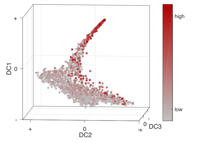
Among continuous phenotypic structured models, recent studies in [47, 48, 49, 50, 51, 52] consider a continuous trait variable that represents the level of cytotoxic drug resistance. This framework allows to explicitly model the heterogeneous response to drugs and effectively study the selection dynamics under microenvironmental constraints and chemotherapy. The asymptotic distributions on the resistance trait space are obtained in [47], and the following works in [49, 51] extend it to include mutations and epimutations. The distribution of resistance levels can be then translated to therapeutic recommendation. The effectiveness of a combination of cytotoxic and cytostatic drugs when cytotoxic resistance emerge is studied in [47]. An optimal combination therapy to eliminate the most resistant clones is proposed in [52]. Moreover, [52] extends the framework that was restricted to solid tumor that is radially symmetric with a fixed boundary [48] to an asymmetric tumor growth model with moving boundary. However, this framework is limited to a single trait variable to a cytotoxic drug.
In this paper we extend the framework of [52] to multi-dimensional resistance trait. We compare our approach that allows for a continuous drug response to more traditional approaches that assume a discrete response to drugs. The paper is organized as follows. In section 2, we introduce a mathematical model for MDR assuming continuous trait variables. We parameterize our model as an extension of a discrete resistance state model in section 2.1 and compute the maximal fitness trait of resistance in section 2.2 for different types of continuum models. This allows us to characterize the cases when the solutions of the continuous models are qualitatively different than the corresponding discrete models. Section 2.3 presents simulation results for the different cases of cytotoxic and cytostatic drugs studied in 2.2. The impact of mutations and epimutations is studied in section 2.4. In section 3 we simulate tumor growth and resistance dynamics subject to MDR on different types of tumors characterized by turnover rates and the proliferating ratios. Our simulations correspond to the discrete MDR models studied by Komarova and Wodarz (2005) [53] and Gardner (2002) [54]. We observe that a combination therapy with multiple cytotoxic drugs is also effective in high turnover tumors using relatively high dosages. Increasing the dosage in low turnover tumor is effective only for certain drug uptake functions. In addition, the drug response function plays a key role in determining the tumor growth dynamics when combination therapy is administered using cell-cycle nonspecific cytotoxic drugs, such as Cyclophosphamide and Doxorubicin. Conclusions and future directions are discussed in section 4.
2 Models of multidrug resistance
Let us consider a cancer growth model under multidrug therapy that depends on an -dimensional phenotype variable . The phenotype variable in the -th direction characterizes the resistance level to the -th drug or the -th drug mechanism, where and represents the fully-sensitive cells and fully-resistant cells to drug , respectively. The value of can be obtained by normalizing the expression level of a gene or a gene cluster that is linked to the cellular levels of drug resistance and proliferative potential, such as ALDH1, CD44, CD117, or MDR1 [38, 55, 56, 57]. The governing equations follows the dynamics of the density of proliferating cells, , and quiescent cells, , as
| (1) | |||||
| (2) |
The first term on the RHS of Eq. (1) is a growth term, , which we assume depends on the resource level with the proliferation rate function as . Also, we assume an exponential growth by considering a constant apoptosis rate for the proliferating cells and for the quiescent cells. To consider a logistic growth, we substitute both terms with a density-dependent apoptosis term , where is the total number of cells
and is a constant that determines the cell capacity.
The net effects of the cytotoxic drugs on the proliferating and quiescent cells are denoted as and , respectively. These terms depend on the marginal drug effects, , the cell death rate due to the -th drug, which is assumed to be a function of the drug concentration . We either consider , where is the drug uptake function of the -th drug, or the exponential kill model [54], , where represents the probability of the cell death due to the -th drug. The net drug effect is modeled as , where is the overall drug effect function that can be taken for the cytotoxic drugs as
| (3) |
and similarly for . The form (3) is valid when is the probability of death due to the -th drug (), and assuming that the drug effects are independent. Dependency between the drugs can be imposed through different choices of , e.g., Copula functions [58] that are used to describe the dependence between random variables using multivariate probability distributions with prescribed marginal distribution functions. In addition to the cytotoxic drugs, we consider cytostatic drugs, which we assume delay the proliferation according to
The net cytostatic drug effect delays the progression of the proliferating cells through the cell cycle. We assume an additive :
Proliferating cells enter the quiescent state at a rate and quiescent cells return to the cycling compartment at a rate . These rates regulate the proliferating portion . To balance a fixed ratio of proliferating cells, namely the proliferating index , the transfer rate can be computed as
The last term in Eq. (1) is a mutation term. We assume that mutations occur at a rate during the proliferation cycle. The mutation is modeled as a integral term with a kernel function . represents the probability of a mother trait mutating to a daughter trait that is taken as an asymmetric exponential function with mutation range , i.e., for , and zero otherwise. Here, is a normalizing constant. This model represents a mutation that gradually increases the resistance level through multiple mutations. A rare mutation that confers a complete drug resistance in a single step can be imposed with a discrete kernel function [50] and a smaller value of .
2.1 Multidrug resistance models parameterized with a binary level of resistance
In this section, we simplify the model given by Eq. (1) to a model that assumes a binary trait space. In this case, cells are either fully-sensitive or fully resistant with respect to each drug, i.e., . To compare the discrete- and continuous-trait models, we parameterize the proliferation and drug function with the parameters related to the microenvironment selection as follows. We denote the proliferation rate of the fully-sensitive cells () as , and assume that the proliferation rate of the fully-resistant cells () is reduced by . With a normalized constant resource level (),
We scale the drug dosage to represent the drug effect on the fully-sensitive cells and assume that the fully-resistant cells do not respond to the drug. This yields a drug uptake function for which and . Hence, the effect of the cytotoxic drug boils down to
See Table 1 for a summary of the fitness parameters.
| parameters | biological meaning |
|---|---|
| maximum proliferation rate | |
| reduced proliferation due to resistance (selection gradient) | |
| maximum apoptosis rate of sensitive cells due to drug |
The resulting model can be written as a dynamical system. For instance, we consider a single () cytotoxic drug affecting the proliferating cells. There exists two cell states: sensitive cells, , and resistant cells, . In this case, the resulting system is
| (4) | |||||
where, , and . In the case of a single cytostatic drug affecting the proliferating cells, the dynamics follows
| (5) | ||||
In case of drugs, the resulting model will involve discrete cell state variables.
The binary models (4) and (5) yield an outcome where either the sensitive cells or the resistant cells dominate the population asymptotically depending on the fitness parameters. In particular, for Eq. (4), with fixed values of and , if the drug dosage is low, , the sensitive cells dominate, but if the drug dosage increases as , the resistant cells dominate the population. The same holds for Eq. (5) with a threshold . If the mutation during treatment is negligible () [53], the thresholds become and for models (4) and (5), respectively.
To connect between models with binary traits and models with continuous traits, we extend the binary models assuming that the proliferation and drug effects are smooth and monotone with respect to . This assumption (although may not always hold) makes it possible to classify continuum scenarios and helps in identifying cases in which the continuous traits dynamics is qualitatively different than the corresponding binary models. Since we only consider proliferating cells, the transfer terms to the quiescent cells are removed from Eq. (1), and we simulate
| (6) |
Starting from the proliferation, we assume that cells that are resistant to cytotoxic drugs use their resources to develop and maintain the drug resistance mechanism [59, 60], that is, . On the domain of , the proliferation function can be characterized according to its concavity. We consider three sample cases: , , and . The cytotoxic drug effect can be modeled similarly. Assuming that apoptosis decreases with an increased level of resistance, we have . Accordingly, we consider three characteristic cases: , , and . The models we consider are summarized in Table 2 and Figure 2.
| concave up | linear | concave down | |
|---|---|---|---|
| (1) | (2) | (3) | |
| (i) | (ii) | (iii) |

2.2 Differentiating models with binary traits from models with continuous traits
To demonstrate the difference between models that are based on binary traits and continuous-traits models, we compute the trait that achieves the maximal fitness of Eq. (6) under different microenvironment conditions. We denote such trait with the maximal growth rate as . Our choices of and in Section 2.1 yield nine cases that are presented in the following list11 1 For simplicity, we compute the maximal fitness trait following the assumption that mutations during treatment are negligible () [53].. We comment that among the nine cases, six cases resemble the discrete model in a sense that the maximal fitness trait is binary, either fully-sensitive or fully-resistant, while three cases allow intermediate trait levels. This demonstrates that in certain circumstances, continuum models are necessary. We first consider the single cytotoxic drug setup that is comparable to the binary model (4). The results are summarized in Table 3.
- 1.
Case (3,i). The maximal growth rate is achieved at that changes its value from to . This case allows an intermediate maximal fitness trait for any drug dosage .
- 2.
Case (3,ii). The maximal growth rate is achieved at . This model increases the maximal trait linearly in terms of the drug dosage when . For , the maximal fitness occurs at .
- 3.
Case (3,iii). The maximal growth rate is either achieved at when , or at when . Since the phenotype distribution asymptotically converges to a delta function centered at or , the overall quality of the solution is similar to the binary-trait model. We also remark that there exists a critical drug dosage at that yields multiple fitness traits.
- 4.
Case (2,i). This model is similar to the case (3,ii), but opposite in the sense that the maximal growth rate is achieved at for , and increases as for .
- 5.
Cases (2,ii), (2,iii), (1,i), (1,ii), and (1,iii). These models also yield a solution that is either concentrated at or , similar to case (3,iii), that is, , where is an indicator function on .
| Case (1) | Case (2) | Case (3) | |
|---|---|---|---|
| (i) | |||
| (ii) | |||
| (iii) |
In addition to cytotoxic drugs, we also consider the drug uptake models in Table 2 for a single cytostatic drug that is comparable to the binary model (5). The maximal fitness traits for the different choices of proliferation rate functions and drug uptake functions are summarized in Table 4.
| Case (1) | Case (2) | Case (3) | |
| (i) | , | , | |
| where | where | ||
| (ii) | , | ||
| where | |||
| (iii) |
2.3 Simulation of continuum model in cytotoxic and cytostatic resistance
In this section, we simulate the model (6) for the cases shown in Table 2 and compare the results with the binary models (4)–(5). For the numerical simulations, we consider the maximal proliferation rate as per day, corresponding to a cell cycle of approximately 25 hours [61, 62]. We also assume that the reduction in proliferation of the resistant cells is per day based on the experiments of non-small lung cancer cells exposed to Erlotinib [59], where the growth rate of resistant cell is reduced by approximately 70%. Experiments with HL60 leukemic cells exposed to vincristine [63] and calculation in [51] further support this assumption. We assume a logistic growth by , where the apoptosis constant that represents the average death rate is taken as . This corresponds to a cell capacity of [63] assuming a solid tumor of size 1cm3 prior to angiogenesis [64] and a tumor cell volume cm3 [65, 66].
case (3,i)
case (3,ii)
case (2,i)
case (2,ii)
case (1,iii)
In Figure 3, we first present the result of the binary-trait model (4) showing that either the fully-resistant or the fully-sensitive cells survive depending on the drug dosage compared to . The total number of sensitive and resistant cells, and , are plotted in log scale with a constant drug dosage up to time . We observe that when , the sensitive cells dominate at , however, when the drug dosage increases to , the resistant cells dominate. When , but close to , the resistant cells will eventually dominate.
In contrast, Figure 4 shows the cancer cell density of the continuous-trait model (6) subject to cytotoxic drug for cases (3,i), (3,ii), (2,i), (2,ii), and (1,iii). We vary the constant cytotoxic drug dosage from to and compute the solution up to time . Case (3,i) always yields an intermediate level of maximal fitness trait of resistance level . Case (3,ii) also yields intermediate levels of when , and otherwise. Alternatively in case (2,i), when , and otherwise. These simulations are consistent with Table 3. Moreover, we observe that the transition from the sensitive to the resistant trait is faster in cases (3,ii) and (2,i) compared with case (3,i), and even more rapid in cases (2,ii) and (1,iii). In particular, cases (2,ii) and (1,iii) result in a distribution that is either concentrated at the fully sensitive or fully resistant trait with a threshold .
(a) binary (b) case (3,i) (c) case (1,iii)
In addition to the resistance trait density, the following quantities of interest are computed. We denote the time that the tumor size as
In addition, the full cell capacity is approximately computed as , where , the time when tumor growth slows down.
(a) (b)
Figure 5 compares the dynamics of the total number of cancer cells using the continuous model (6) and binary model (4) up to . The times and are delayed as the cytotoxic drug dosage increases. However, in the binary model, the results are essentially identical when the dosage is relatively high as . Moreover, the tumor size of approximate full capacity in the continuum case (3,i) is gradually reduced as the drug dosage increases, which is not the case in the binary-trait model and case (1,iii). The results of and with respect to the cytotoxic drug dosage shown in Figure 6, where the distinction between the binary and continuum models are more apparent. The binary model yields an identical result after the drug dosage increases above , while the continuum models show a gradual change depending on the drug dosage. We observe that with our model parameters the results are more sensitive to the choice of the drug effect function (case i, ii, iii) than to the proliferation function (case 1, 2, 3).
case (3,i)
case (2,ii)
case (1,iii)
(a) (b)
The case of a cytostatic drug comparing the continuous model (6) and binary model (5) is shown in Figures 7 and 8. The resistance trait distribution considering cases (3,i), (2,ii), and (1,iii) are plotted in Figure 7. The intermediate resistance level of maximal fitness is achieved in case (3,i) for all drug dosages at , where , similar to the results of using cytotoxic drugs. We also observe a binary outcome either at the most sensitive or the most resistant trait depending on the drug dosage threshold . The time and approximate capacity are shown in Figure 8. In contrast to the cytotoxic drug case, the binary model also shows a gradual change as a function of the drug dosage. Still, the results obtained by the binary and continuous models are different.
2.4 Epimutation in drug resistance
In this section, we investigate the effect of epimutation on the drug resistance dynamics of cancer cells. Phenotypic variants in cancer cell populations emerge not only from genetic mutations, but also due to epimutations. Epimutations are heritable changes in gene expression that do not alter the DNA, but contribute to the phenotypic instability [67, 68, 69, 70, 71]. Recent experiments demonstrate that such non-genetic instability and phenotypic variability allows cancer cells to reversibly transit between different phenotypic states [72, 63, 73] and contributes to development of resistance to cytotoxic drugs [75, 76]. In the continuous phenotypic models, epimutation can be readily modeled as a diffusion term assuming that random epimutations yield infinitesimally small phenotypic modifications [77, 78, 51]. The dynamics of proliferating cells in Eq. (6) with an epimutation rate can be written as
| (7) |
The asymptotic distribution of the continuum model with epimutation for the case (3,i) is derived in [51]. Here, we study the effect of epimutation in different continuum models.
case (3,i)
case (1,iii)
cytotoxic drug cytostatic drug
Figure 9 shows the resistance trait density with epimutation using Eq. (7) corresponding to cases (3,i) and (1,iii) when the rate of epimutation is . Although the maximum fitness trait is similar to the results without epimutations in Figure 4, the phenotypic instability yields a significantly more heterogeneous population, not only in case (3,i), where the maximal fitness trait is intermediate, but also in case (1,iii), where the distribution becomes a Dirac-delta function at the boundary trait without epimutations.
(a) (b)
We now study the effect of epimutations on the time that the tumor size reaches a certain size in different models subject to cytotoxic drugs. In particular, we compare epimutations with regular mutations. Figure 10 shows the time of relapse using the binary models (4)–(5) with and without mutations of rate initiated from and . In general, mutations accelerate the relapse time by increasing the proportion of resistant cells under a sufficiently high dosage. We remark that this is similar in the continuum models, when using the asymmetric mutation kernel described section 2. However, Figures 11 and 12 show that epimutations in the continuum model (7) often delay the relapse time. We consider two initial conditions: (a) , where we set and so that and ; and (b) a linear distribution , which has a larger population of resistant cells.
(a) (b)
In Figure 11, using the epimutation model (7) subject to cytotoxic drugs, we observe that is delayed with the initial condition , especially in case (iii) with a larger rate . However, epimutations with initial condition accelerate the relapse in case (i), and also for a certain range of drug dosages in case (iii). For a higher cytotoxic dosage in case (iii), the relapse time is again delayed. Similarly, Figure 12 shows the effect of epimutations on the conitnuum model (7) subject to cytostatic drugs. Compared with the cytotoxic drugs, resistance to cytostatic drugs is less affected by epimutation especially when starting with the initial condition . However, an earlier relapse is observed with the initial condition in both models (i) and (iii).
In conclusion, compared with regular mutations that give advantage to tumor growth under drug administration, epimutations have more diverse effects that can either promote or slow down tumor growth depending on other circumstances, including the drug uptake function and the initial conditions.
3 Simulating tumor growth under multidrug therapy
In this section we demonstrate how our continuous phenotype structured modeling framework can be used to study MDR. The impact of the tumor’s turnover rate and the proliferating fraction of cancer cells have been studied within a discrete phenotype framework by Komarova and Wodarz (2005) [53] and by Gardner (2002) [54]. Here, we compare the results obtained with our approach with the conclusions of [53, 54].
3.1 Multidrug resistance: tumor turnover rate
The impact of the turnover rate in tumor growth and resistance dynamics has been studied by Komarova and Wodarz (2005) [53]. Their model assumes two discrete states for cytotoxic drugs, adding to discrete resistance levels. The model assumes a constant growth rate , a constant death rate , and is independent of the cell-cycle. Komarova and Wodarz conclude that when comparing tumors of identical sizes at detection, high turnover tumors () have a higher probability of treatment failure than low turnover tumors (). Moreover, a combination therapy () is less likely to have an advantage over single-drug therapy in tumors with high turnover rates. In contrast, in the continuum models we show that depending on the proliferation and drug response functions, a combination therapy to high turnover tumor can be more effective than a single drug treatment. This is the case with relatively higher dosages when the drug uptake follows model (i). In addition, increasing the dosage in low turnover tumors is effective in delaying the tumor relapse when the drug uptake follows model (i), but not in model (iii).
(iii,iii) (i,iii) (i,i)

The simulation we present is computed using the continuum model (6) with the different drug response functions in Table 2. As in [53], we assume a constant proliferation rate , and model the high and low turnover tumor by setting and , respectively. The cytotoxic drug effect is taken as , where we consider a single parameter for the drug dosage, and with the uptake functions . We consider the drug dosages around in high turnover tumors and in low turnover tumors.
Figure 13 presents the cell density in the resistance trait space using the continuum model (6) subject to a combination therapy using two cytotoxic drugs (). We consider a high turnover tumor with the uptake functions of cases (i,i), (i,iii), and (iii,iii), and set the drug dosage as . The distributions shown are cancer cell densities in log scale, , at time . The marginalized distribution in each resistance trait is similar to the results of section 2.3, where case (iii) yields more localized distributions near in relatively higher dosages compared to case (i).
We now compare the responses of high and low turnover tumors with respect to the number of drugs in the continuous models. Figure 14 shows the total number of cells up to for an increasing number of drugs , and increasing drug dosages. We choose case (i) for the drug uptake function. As expected, we observe a delayed growth with an increased number of drugs and increased dosages. While increasing the number of drugs is not effective in high turnover tumors in the model of [53], it is effective in the continuum model (6) with the drug update model (i) and high dosages . Figure 15 compares the total number of cells in four different continuum models, combining the drug effect (case (i), (iii)) and the turnover rate (, ). We observe that increasing the drug dosage over a certain threshold is less likely to delay the relapse time in low turnover tumor for which the drug uptake follows case (iii). It is effective in drug uptake case (i).
case (iii) case (i)

Finally, Figure 16 shows the effect of increasing the number of drugs assuming a logistic growth model by taking in Eq. (6). In this case, the dynamics does not depend on the turnover rate except that the cell capacity changes. The results are shown for , and we remark that taking shows essentially no difference. However, the relapse does depend on the choice of a continuum model. Increasing the number of drugs delays the relapse in both cases (i) and (iii), but more so in case (iii) compared with (i).
We conclude that in addition to the turnover rate, the drug uptake function of the continuum model is also important in controlling the outcome of the treatment. In particular, a combination therapy with multiple drugs is effective not only in low turnover tumors, but also in high turnover tumors with the drug uptake case (i). Moreover, a high cytotoxic drug dosage in low turnover tumor with case (iii) is less effective than case (i). The drug uptake function is often more important than the turnover rate in determining the outcome of the tumor growth and relapse, particularly with a logistic growth condition.
3.2 Multidrug resistance: heterogeneity due to the proliferating index
Gardner (2002) [54] proposed an individually tailored model based on the tumor cell kinetics of patients following heterogeneous colonies of proliferating and quiescent cells. This study considered multidrug resistance to six specific drugs, including two cell-cycle specific (CS) cytotoxic drugs, 5-Fluorouracil and Methotrexate, that only affect the proliferating cells; two cell-cycle nonspecific (nCS) cytotoxic drugs, Cyclophosphamide and Doxorubicin, that kill both proliferating and quiescent cells; and two cytostatic drugs, Tamoxifen and Herceptin. The model assumed discrete levels of resistance in addition to the parameters of cell division rates, apoptotic rates, response to drugs, and evolution of drug resistance. It then used the discrete model to predict drug combinations and schedules that are likely to be effective in reducing the tumor size.
The governing system in [54] assumes three discrete drug resistance levels, , for each of the six drugs, and it is similar to Eqs. (1)-(2):
| (8) | ||||
Here and are defined on discrete resistance levels. In addition, includes the effect of apoptosis of proliferating cells of rate , the quiescent cells die as a result of necrosis of rate , and denotes the mutation term similar to Eq. (1) [54]. The transfer rates from the quiescent cells to the proliferating cells to balance a fixed ratio of proliferating cells is . We denote the CS cytotoxic drugs as and , the nCS cytotoxic drugs as and , and the cytostatic drugs as and . The drug effects are modeled using the exponential kill model [81] as for the CS cytotoxic drug (), for the nCS cytotoxic drug (), and for the cytostatic drug (), where and the domain of resistance trait is taken at three discrete levels . The net drug effects are taken as
| (9) | |||
Figure 17 shows the three discrete levels of drug effect using the dosages , …, from [54] (see A). We note that although Gardner considers three levels of resistance, the cells with sensitive levels and of , and have similar response to the drug. Moreover, the exponential kill model of , , , and based on the concavity can be classified as our case (iii), and and as case (ii). In the following simulations, we assume that the proliferation and the drug effects in Eqs. (1)–(2) follow the models as in Table 2 with the net drug effect as in (9), and compare the results with the discrete model (8). See A for the model parameters.
no drug

[, ] [, ] [,…,]

Figure 18 compares the result of the discrete model (8) and the continuum model (1)–(2), in particular with regards to the drug . Shown is the cell distribution on the resistance trait space of drug in log scale22 2 , where is the vector of except the -th index and is its domain. , when using no drug, a single drug , and all 6 drugs. Here, the continuum model is taken as the exponential kill model that can be classified as cases (iii) and (ii). As expected from the shape of the uptake function in Figure 17, the distribution in the trait space is concentrated at the boundary traits, similarly to the discrete model. However, the continuum model predict emerging cells with intermediate levels of resistance, and the degree of heterogeneity in the resistance level can be quantitatively computed.
Figure 19 compares the sensitivity of the tumor size with respect to the drug dosage between the continuum model (1)–(2) and the discrete model (8). For comparison, we plot the normalized total number of cells in log scale at time that is normalized by the mean. Here, two drugs are applied, either or , with different weighted dosages , where . The results show that the tumor size in the continuum model is more sensitive to the drug dosage, with variation of a larger order of magnitude compared with the results of the discrete model. In addition, the effects of drugs , , and in the discrete model are binary depending on whether the drug is applied () or not (). In contrast, the continuum model shows a gradual decay when increasing the dosage. Figure 19 also shows the total number of cells when all six drugs are applied. We observe that significantly depends on the choice of model, as the tumor size varies by two orders of magnitudes around .
(a) (b) (c)
Figure 20 compares the mean resistance level33 3 , where and is the vector of except the -th index and is its domain. up to when all 6 drugs are applied. While the mean resistance level in implies the dominating resistance to the -th drug, we observe distinct results in different models. First, using the discrete model (8), the resistance level in each drug eventually converges to the most resistant cells . This implies that the surviving cancer cells are only the ones that are fully resistant to all six drugs. However, the continuum model (1)–(2) shows a more gradual increase of resistance. Moreover, the resistance to nCS cytotoxic drugs develops more rapidly in case (iii) than in case (i). On the other hand, resistance to CS cytotoxic drugs and to cytostatic drugs is more sensitive to the drug application in case (i) that in case (iii). We finally comment that shows similar dynamics when using drugs with the same mechanism, that is, the results with drugs , , and are similar to , , and , respectively.

Gardner (2002) [54] presents the effect of different drug combinations particularly to cancer cells with different proliferating proportions . Figure 21 shows simulations of the total number of tumor cells with a highly proliferating index () and a low proliferating index (). We demonstrate that the drug response function plays a key role in determining the tumor growth dynamics using certain combination therapies that often involve the nCS cytotoxic drugs ( and ). In general, the drug combinations that includes CS cytotoxic drugs ( and ) are more effective in highly proliferating tumors. In the discrete model (8), the drug combinations without the CS cytotoxic drugs show no difference. However, in the continuum model (1)–(2), the highly proliferating cancer cells show disadvantage under drug combinations without CS cytotoxic drugs, which reveals a possible internal dependency between the drugs.
We observe that the choice of continuum model is critical to the emerging drug response. For an effective individually-tailored cancer modeling, these results stress the importance of identifying an appropriate model depending on the drug response of each individuals.
4 Conclusion
In this paper we propose a mathematical model for multidrug resistance, assuming a continuous resistance phenotype space. The multidrug resistance trait variable represents the level of resistance to various drugs including cell-cycle specific and nonspecific cytotoxic drugs, as well as cytostatic drugs. We classify the proliferation and drug uptake functions and identify the cases where the continuum model results in an intermediate maximal fitness resistance, i.e., the cases in which the continuum and discrete models are essentially different. Thus, by observing the proliferation and drug effects, we can predict when the continuum models are different than the corresponding discrete models. We study the effect of epimutation on the cytotoxic and cytostatic resistance traits. In contrast to standard mutations that are associated with an early relapse, epimutations may either accelerate or delay the relapse time. We demonstrate such effects on different continuum models, initial preexisting resistance ratios, and types of drugs.
We use our approach to revising the works of Komarova and Wodarz (2005) [53] and the Gardner (2002) [54]. Following [53], we study the impact of the turnover rate on tumor growth and drug response. We verify the effectiveness of a combination therapy with multiple cytotoxic drugs in low turnover tumors and also in high turnover tumors with a drug uptake function of case (i) under high drug dosages. Increasing the cytotoxic drug dosage delays the relapse in tumor that the drug uptake follows case (iii), but not in low turnover tumor with case (i), thus in particular in such cases, the dosage should be carefully chosen. Moreover, the choice of a drug uptake function is shown to have a higher impact than the turnover rate under a logistic growth condition. These results provide new insights on the dynamics beyond what is accessible by (and in certain cases even contradictory to) the discrete-trait model of [53].
The second example we studied followed [54] by considering three different types of drugs: cell cycle specific and nonspecific cytotoxic drugs, and cytostatic drugs. We demonstrated that the size of the tumor is more sensitive to the drug dosage in the continuum models compared with the model of [54]. In addition, a drug combination without the cell cycle specific cytotoxic drug shows no disadvantage in highly proliferating tumors in the discrete model, which is not the case in the continuum models. We conclude that the dynamics of the cancer cell population including the time of relapse and the resistance profile significantly depends on the choice of (continuum) models, in addition to the turnover rate and the proliferation index. Thus, it is critical to select appropriate multidrug resistance models depending on the drug response of each individuals, to accomplish an effective individually-tailored cancer modeling framework and a corresponding optimal drug therapy.
Our future work includes deriving a continuum model from high-dimensional data that will be preprocessed with data analysis techniques. In addition, modeling the dependency structure of multiple drugs and investigating its effect on the resistance dynamics is another challenging topic. Finally, due to its dimensionality, simulation of multidrug resistance model requires developing an efficient numerical method that balances computational cost and accuracy. This will be addressed with adaptive numerical methods that take advantage of the underlying low dimensional structure of the solution.
Acknowledgments
The work of DL was supported in part by the National Science Foundation under Grant Number DMS-1713109 and by the Jayne Koskinas Ted Giovanis Foundation.
Appendix A Parameters of simulation
- 1.
- 2.
- 3.
- 4.
Necrosis rate of the quiescent cells: [88].
- 5.
where is the amount of drug built up from previous drug applications and the parameters for drug administration are as follows [89, 90, 91].
-Periods of drug administration: , , .
-Duration of drug administration: h, h, h.
-Drug dosage scaled for and : , , , , , .
- 6.
Mutation rate: [26].
References
References
- [1] M. M. Gottesman, Mechanisms of cancer drug resistance., Annu Rev Med 53 (2002) 615–627.
- [2] M. M. Gottesman, T. Fojo, S. E. Bates, Multidrug Resistance in Cancer: Role of ATP-Dependent Transporters, Nat. Rev. Cancer 2 (1) (2002) 48–58.
- [3] V. Fodal, M. Pierobon, L. Liotta, E. Petricoin, Mechanisms of cell adaptation: when and how do cancer cells develop chemoresistance?, Cancer J. 17 (2) (2011) 89–95.
- [4] S. Byler, S. Goldgar, S. Heerboth, M. Leary, G. Housman, K. Moulton, S. Sarkar, Genetic and epigenetic aspects of breast cancer progression and therapy, Anticancer Res. 34 (3) (2014) 1071–1077.
- [5] S. Byler, S. Sarkar, Do epigenetic drug treatments hold the key to killing cancer progenitor cells?, Epigenomics 6 (2) (2014) 161–165.
- [6] C. L. Chaffer, R. A. Weinberg, A perspective on cancer cell metastasis, Science 331 (6024) (2011) 1559–1564.
- [7] S. Sarkar, G. Horn, K. Moulton, A. Oza, S. Byler, S. Kokolus, M. Longacre, Cancer development, progression, and therapy: an epigenetic overview, Int. J. Mol. Sci. 14 (10) (2013) 21087–21113.
- [8] C. Pouchol, J. Clairambault, A. Lorz, E. Trélat, Asymptotic analysis and optimal control of an integro-differential system modelling healthy and cancer cells exposed to chemotherapy, Journal de Mathématiques Pures et Appliquées (2018) 1–47.
- [9] J. M. Greene, J. L. Gevertz, E. D. Sontag, A mathematical approach to differentiate spontaneous and induced evolution to drug resistance during cancer treatment, bioRxiv https://doi.org/10.1101/235150.
- [10] J.-P. Gillet, M. M. Gottesman, Mechanisms of Multidrug Resistance in Cancer, Methods Mol Biol 596 (2010) 47–76.
- [11] J. H. Goldie, A. J. Coldman, A mathematical model for relating the drug sensitivity of tumors to their spontaneous mutation rate, Cancer Treat. Rep. 63 (1979) 1727–1733.
- [12] J. H. Goldie, A. J. Coldman, A model for resistance of tumor cells to cancer chemotherapeutic agents, Math. Biosci. 65 (1983a) 291–307.
- [13] J. H. Goldie, A. J. Coldman, Quantative model for multiple levels of drug resistance in clinical tumors, Cancer Treat. Rep. 67 (1983b) 923–931.
- [14] Y. Iwasa, M. A. Nowak, F. Michor, Evolution of resistance during clonal expansion, Genetics 172 (2006) 2557–2566.
- [15] M. Kimmel, A. Swierniak, A. Polanski, Infinite-dimensional model of evolution of drug resistance of cancer cells, J. Math. Syst. Estim. Control 8 (1998) 1–16.
- [16] N. Komarova, Stochastic modeling of drug resistance in cancer, Theor. Popul. Biol. 239 (3) (2006) 351–366.
- [17] F. Michor, M. A. Nowak, Y. Iwasa, Evolution of Resistance to Cancer Therapy, Curr. Pharm. Des. 12 (2006) 261–271.
- [18] B. G. Birkhead, E. M. Rakin, S. Gallivan, L. Dones, R. D. Rubens, A mathematical model of the development of drug resistance to cancer chemotherapy, Eur. J. Cancer Clin. Oncol. 23 (1987) 1421–1427.
- [19] C. Tomasetti, D. Levy, An elementary approach to modeling drug resistance in cancer, Math. Biosci. Eng. 7 (2010) 905–918.
- [20] A. R. Anderson, M. Chaplain, Continuous and discrete mathematical models of tumor-induced angiogenesis., Bull. Math. Biol. 60 (5) (1998) 857–899.
- [21] O. Trédan, C. M. Galmarini, K. Patel, I. F. Tannock, Drug resistance and the solid tumor microenvironment, J. Natl. Cancer Inst. 99 (2007) 1441–1454.
- [22] A. Wu, K. Loutherback, G. Lambert, L. Estévez-Salmerón, T. D. Tlsty, R. H. Austin, J. C. Sturm, Cell motility and drug gradients in the emergence of resistance to chemotherapy, Proc. Natl. Acad. Sci. 110 (40) (2013) 16103–16108.
- [23] O. Lavi, M. M. Gottesman, D. Levy, The dynamics of drug resistance: A mathematical perspective, Drug Resist. Updates 15 (1-2) (2012) 90–97.
- [24] J. Foo, F. Michor, Evolution of resistance to anti-cancer therapy during general dosing schedules, J. Theor. Biol. 263 (2010) 179–188.
- [25] T. Roose, S. J. Chapman, P. K. Maini, Mathematical models of avascular tumor growth, Siam Review 49 (2) (2007) 179–208.
- [26] J. H. Goldie, A. J. Coldman, Drug resistance in cancer: mechanisms and models, Cambridge University Press, first edn., 1998.
- [27] V. Panagiotopoulou, G. Richardson, O. E. Jensen, C. Rauch, On a biophysical and mathematical model of Pgp-mediated multidrug resistance: understanding the “space-time” dimension of MDR, Eur. Biophys. J. 39 (2010) 201–211.
- [28] A. Swierniak, M. Kimmel, J. Smieja, Mathematical modeling as a tool for planning anticancer therapy, Eur. J. Pharmacol. 625 (1-3) (2009) 108–121.
- [29] Y. Saeys, S. Van Gassen, B. N. Lambrecht, Computational flow cytometry: Helping to make sense of high-dimensional immunology data, Nature Reviews Immunology 16 (7) (2016) 449–462.
- [30] A. Wagner, A. Regev, N. Yosef, Revealing the vectors of cellular identity with single-cell genomics, Nature Biotechnology 34 (11) (2016) 1145–1160.
- [31] I. C. Macaulay, V. Svensson, C. Labalette, L. Ferreira, F. Hamey, T. Voet, S. A. Teichmann, A. Cvejic, Single-Cell RNA-Sequencing Reveals a Continuous Spectrum of Differentiation in Hematopoietic Cells, Cell Reports 14 (4) (2016) 966–977.
- [32] M. J. T. Stubbington, O. Rozenblatt-Rosen, A. Regev, S. A. Teichmann, Single-cell transcriptomics to explore the immune system in health and disease, Science 358 (6359) (2017) 58–63.
- [33] L. Velten, S. F. Haas, S. Raffel, S. Blaszkiewicz, S. Islam, B. P. Hennig, C. Hirche, C. Lutz, E. C. Buss, D. Nowak, T. Boch, W. K. Hofmann, A. D. Ho, W. Huber, A. Trumpp, M. A. Essers, L. M. Steinmetz, Human haematopoietic stem cell lineage commitment is a continuous process, Nature Cell Biology 19 (4).
- [34] S. C. Bendall, E. F. Simonds, P. Qiu, E.-a. D. Amir, P. O. Krutzik, R. V. Bruggner, R. Melamed, A. Trejo, O. I. Ornatsky, R. S. Balderas, S. K. Plevritis, K. Sachs, D. Pe, S. D. Tanner, G. P. Nolan, Single-Cell Mass Cytometry of Differential Immune and Drug Responses Across a Human Hematopoietic Continuum, Science 332 (6030) (2011) 687–696.
- [35] A. H. Rizvi, P. G. Camara, E. K. Kandror, T. J. Roberts, I. Schieren, T. Maniatis, R. Rabadan, Single-cell topological RNA-seq analysis reveals insights into cellular differentiation and development, Nature Biotechnology 35 (6) (2017) 551–560.
- [36] M. Mojtahedi, A. Skupin, J. Zhou, I. G. Castaño, R. Y. Leong-Quong, H. Chang, K. Trachana, A. Giuliani, S. Huang, Cell Fate Decision as High-Dimensional Critical State Transition, PLoS Biology 14 (12) (2016) 1–28.
- [37] A. Grover, A. Sanjuan-Pla, S. Thongjuea, J. Carrelha, A. Giustacchini, A. Gambardella, I. Macaulay, E. Mancini, T. C. Luis, A. Mead, S. E. W. Jacobsen, C. Nerlov, Single-cell RNA sequencing reveals molecular and functional platelet bias of aged haematopoietic stem cells., Nature communications 7 (2016) 11075.
- [38] E.-a. D. Amir, K. L. Davis, M. D. Tadmor, E. F. Simonds, H. Levlne, Jacob, S. C. Bendall, D. K. Shenfeld, S. Krishnaswamy, G. P. Nolan, D. Pe’er, viSNE enables visualization of high dimensional single-cell data and reveals phenotypic heterogeneity of leukemia, Nat Biotechnol. 31 (6) (2013) 545–552.
- [39] V. van Unen, T. Höllt, N. Pezzotti, N. Li, M. J. T. Reinders, E. Eisemann, F. Koning, A. Vilanova, B. P. F. Lelieveldt, Visual analysis of mass cytometry data by hierarchical stochastic neighbour embedding reveals rare cell types, Nature Communications 8 (1) (2017) 1740.
- [40] L. Haghverdi, F. Buettner, F. J. Theis, Diffusion maps for high-dimensional single-cell analysis of differentiation data, Bioinformatics 31 (18) (2015) 2989–2998.
- [41] S. Nestorowa, F. K. Hamey, B. Pijuan Sala, E. Diamanti, M. Shepherd, E. Laurenti, N. K. Wilson, D. G. Kent, B. Gottgens, B. P. Sala, E. Diamanti, M. Shepherd, E. Laurenti, N. K. Wilson, D. G. Kent, G. Berthold, A single-cell resolution map of mouse hematopoietic stem and progenitor cell differentiation, Blood 128 (8) (2016) 20–32.
- [42] F. Buggenthin, F. Buettner, P. S. Hoppe, M. Endele, M. Kroiss, M. Strasser, M. Schwarzfischer, D. Loeffler, K. D. Kokkaliaris, O. Hilsenbeck, T. Schroeder, F. J. Theis, C. Marr, Prospective identification of hematopoietic lineage choice by deep learning, Nature Methods 14 (4) (2017) 403–406.
- [43] P. S. Stumpf, R. C. Smith, M. Lenz, A. Schuppert, F. J. Müller, A. Babtie, T. E. Chan, M. P. Stumpf, C. P. Please, S. D. Howison, F. Arai, B. D. MacArthur, Stem Cell Differentiation as a Non-Markov Stochastic Process, Cell Systems 5 (3) (2017) 268–282.
- [44] D. Julie, B. Raymond, B. Danuta, ALDH1 as a Functional Marker of Cancer Stem and Progenitor Cells, Stem Cells and Development 18 (1) (2009) 17–26.
- [45] G. Schiebinger, J. Shu, M. Tabaka, B. Cleary, V. Subramanian, A. Solomon, S. Liu, S. Lin, P. Berube, L. Lee, J. Chen, J. Brumbaugh, P. Rigollet, K. Hochedlinger, R. Jaenisch, A. Regev, E. Lander, Reconstruction of developmental landscapes by optimal-transport analysis of single-cell gene expression sheds light on cellular reprogramming., bioRxiv, https://doi.org/10.1101/191056 .
- [46] H. Cho, K. Ayers, L. DePills, Y.-H. Kuo, J. Park, A. Radunskaya, R. Rockne, Modeling acute myeloid leukemia in a continuum of differentiation states, Letters in Biomathematics (2018) 1–30.
- [47] A. Lorz, T. Lorenzi, M. E. Hochberg, J. Clairambault, B. Perthame, Populational adaptive evolution, chemotherapeutic resistance and multiple anti-cancer therapies, Esaim Math Model Numer Anal 47 (2013) 377–399.
- [48] A. Lorz, T. Lorenzi, J. Clairambault, A. Escargueil, B. Perthame, Modeling the Effects of Space Structure and Combination Therapies on Phenotypic Heterogeneity and Drug Resistance in Solid Tumors, Bull Math Biol 77 (2015) 1–22.
- [49] J. Greene, O. Lavi, M. M. Gottesman, D. Levy, The Impact of Cell Density and Mutations in a Model of Multidrug Resistance in Solid Tumors, Bull. Math. Biol. 74 (2014) 627–653.
- [50] H. Cho, D. Levy, Modeling the dynamics of heterogeneity of solid tumors in response to chemotherapy, Bull. Math. Biol. 79 (12) (2017) 2986–3012.
- [51] T. Lorenzi, R. H. Chisholm, J. Clairambault, Tracking the evolution of cancer cell populations through the mathematical lens of phenotype-structured equations, Biology Direct 11 (43) (2016) 1–17.
- [52] H. Cho, D. Levy, Modeling the chemotherapy-induced selection of drug-resistant traits during tumor growth, J. Theor. Biol. 436 (7) (2018) 120–134.
- [53] N. L. Komarova, D. Wodarz, Drug resistance in cancer: principles of emergence and prevention., Proc. Natl. Acad. Sci. 102 (27) (2005) 9714–9719.
- [54] S. N. Gardner, Modeling multi-drug chemotherapy: Tailoring treatment to individuals, Journal of Theoretical Biology 214 (2) (2002) 181–207.
- [55] D. Hanahan, R. A. Weinberg, Hallmarks of cancer: the next generation, Cell 144 (5) (2011) 646–674.
- [56] J. P. Medema, Cancer stem cells: the challenges ahead, Nat. Cell Biol. 15 (4) (2013) 338–344.
- [57] A. O. Pisco, S. Huang, Non-genetic cancer cell plasticity and therapy-induced stemness in tumour relapse: ’What does not kill me strengthens me’, British Journal of Cancer 112 (11) (2015) 1725–1732.
- [58] R. B. Nelsen, An Introduction to Copulas, New York: Springer, 1999.
- [59] S. M. Mumenthaler, J. Foo, N. C. Choi, N. Heise, K. Leder, D. B. Agus, W. Pao, F. Michor, P. Mallick, The Impact of Microenvironmental Heterogeneity on the Evolution of Drug Resistance in Cancer Cells, Cancer Informatics 14 (2015) 19–31.
- [60] K. Wosikowski, J. A. Silverman, P. Bishop, J. Mendelsohn, S. E. Bates, Reduced growth rate accompanied by aberrant epidermal growth factor signaling in drug resistant human breast cancer cells, Biochimica et Biophysica Acta 1497 (2) (2000) 215–226.
- [61] G. Steel, L. Lamerton, The growth rate of human tumours, Br. J. Cancer 20 (1) (1966) 74–86.
- [62] P. Calabresi, P. S. Schein, Medical Oncology : Basic principles and clinical management of cancer, New York : McGraw-Hill, second edn., 1993.
- [63] A. O. Pisco, A. Brock, J. Zhou, A. Moor, M. Mojtahedi, D. Jackson, S. Huang, Non-darwinian dynamics in therapy-induced cancer drug resistance, Nat. Commun 4 (2013) 2467.
- [64] A. R. Anderson, A hybrid mathematical model of solid tumour invasion: The importance of cell adhesion, Math. Med. Biol. 22 (2) (2005) 163–186.
- [65] J. J. Casciari, S. V. Sotirchos, R. M. Sutherland, Variation in tumour cell growth rates and metabolism with oxygen-concentration, glucose-concentration and extracellular pH, J. Cell. Physiol. 151 (1992) 386–394.
- [66] J. Folkman, M. Hochberg, Self-regulation of growth in three dimensions, J. Exp. Med. 138 (1973) 745–753.
- [67] A. Brock, H. Chang, S. Huang, Non-genetic heterogeneity - a mutation-independent driving force for the somatic evolution of tumours, Nat. Rev. Genet. 10 (5) (2009) 336–342.
- [68] R. Glasspool, J. M. Teodoridis, R. Brown, Epigenetics as a mechanism driving polygenic clinical drug resistance, Br. J. Cancer 94 (8) (2006) 1087–1092.
- [69] P. B. Gupta, C. M. Fillmore, G. Jiang, S. D. Shapira, K. Tao, C. Kuperwasser, E. S. Lander, Stochastic state transitions give rise to phenotypic equilibrium in populations of cancer cells, Cell 146 (4) (2011) 633–644.
- [70] J. R. Newman, S. Ghaemmaghami, J. Ihmels, D. K. Breslow, M. Noble, J. L. DeRisi, J. S. Weissman, Single-cell proteomic analysis of s. cerevisiae reveals the architecture of biological noise, Nature 441 (7095) (2006) 840–846.
- [71] A. Raj, A. van Oudenaarden, Nature, nurture, or chance: stochastic gene expression and its consequences, Cell 135 (2) (2008) 216–226.
- [72] H. H. Chang, P. Y. Oh, D. E. Ingber, S. Huang, Multistable and multistep dynamics in neutrophil differentiation, BMC Cell Biol. 7 (11) (2006) 1–12.
- [73] S. V. Sharma, D. Y. Lee, B. Li, M. P. Quinlan, F. Takahashi, S. Maheswaran, U. McDermott, N. Azizian, L. Zou, M. A. Fischbach, A chromatin-mediated reversible drug-tolerant state in cancer cell subpopulations, Cell 141 (1) (2010) 69–80.
- [74] R. H. Chisholm, T. Lorenzi, A. Lorz, A. K. Larsen, L. N. d. Almeida, A. Escargueil, J. Clairambault, Emergence of Drug Tolerance in Cancer Cell Populations: An Evolutionary Outcome of Selection, Nongenetic Instability, and Stress-Induced Adaptation, Cancer Research 75 (6) (2015) 930–939.
- [75] R. H. Chisholm, T. Lorenzi, J. Clairambault, Cell population heterogeneity and evolution towards drug resistance in cancer: biological and mathematical assessment, theoretical treatment optimization, Biochimica et Biophysica Acta (BBA) 1860 (11) (2016) 2627–2645.
- [76] S. Huang, Genetic and non-genetic instability in tumor progression: link between the fitness landscape and the epigenetic landscape of cancer cells, Cancer Metastasis Rev. 32 (3–4) (2013) 423–448.
- [77] C. Becker, J. Hagmann, J. Müller, D. Koenig, O. Stegle, K. Borgwardt, D. Weigel, Spontaneous epigenetic variation in the arabidopsis thaliana methylome, Nature 480 (2011) 245–249.
- [78] N. E. Navin, Cancer genomics: one cell at a time, Genome Biol. 15 (8) (2014) 452.
- [79] W. D. Stein, W. D. Figg, W. Dahut, A. D. Stein, M. B. Hoshen, D. Price, S. E. Bates, T. Fojo, Tumor Growth Rates Derived from Data for Patients in a Clinical Trial Correlate Strongly with Patient Survival: A Novel Strategy for Evaluation of Clinical Trial Data, The Oncologist 13 (10) (2008) 1046–1054.
- [80] M. Rosa Durán, A. Podolski-Renić, A. Álvarez-Arenas, J. Dinić, J. Belmonte-Beitia, M. Pešić, V. M. Pérez-García, Transfer of Drug Resistance Characteristics Between Cancer Cell Subpopulations: A Study Using Simple Mathematical Models, Bulletin of Mathematical Biology 78 (6) (2016) 1218–1237.
- [81] S. N. Gardner, A mechanistic, predictive model of dose response curves for cell cycle phase-speciffc and non-speciffc drugs, Cancer Res. 60 (2000) 1417–1425.
- [82] G. G. Steel, The Growth Kinetics of tumors, Oxford University Press, 1977.
- [83] F. L. Baker, L. J. Sanger, R. W. Rodgers, K. Jabboury, O. R. Mangini, Cell proliferation kinetics of normal and tumor tissue in vitro: quiescent reproductive cells and the cycling reproductive fraction, Cell Prolif. 28 (1995) 1–15.
- [84] A. C. Begg, Basic Clinical Radiobiology, chap. Cell proliferation in tumors, New York: Oxford University Press, Inc., 14–22, 1997.
- [85] J. C. Panetta, A mathematical model of drug resistance: heterogeneous tumors, Math. Biosci. 147 (1) (1997) 41–61.
- [86] B. I. Lord, Stem Cells, chap. Biology of haemopoietic stem cell, San Diego: Academic Press, 401–422, 1997.
- [87] T. Papayannopoulou, J. Abkowitz, A. D’andrea, Hematology, Basic Principles and Practice, chap. Biology of Erythropoiesis, erythroid differentiation, and maturation, New York: Churchill Livingstone, 203, 2000.
- [88] J. T. Leith, S. Michelson, Changes in the extents of viable and necrotic tissue, interstitial fluid pressure, and proliferation kinetics in clone. A human colon tumour xenografts as a function of tumour size, Cell Prolif. 27 (12) (1994) 723–739.
- [89] B. A. Chabner, Cancer, chap. Anticancer drugs, Philadelphia: Lippincott, 325–340, 1993.
- [90] M. M. Goldenberg, Trastuzumab, a recombinant DNA-derived humanized monoclonal antibody, a novel agent for the treatment of metastatic breast cancer, Clin. Ther. 21 (2) (1999) 309–318.
- [91] Tamoxifen monograph, http://www.bccancer.bc.ca/drug-database-site/Drug%20Index/Tamoxifen_monograph_1May2017.pdf, 2017.