跳到论文正文
W Papers独立论文阅读器 arXiv:1806.07549 论文正文 计算阅读时间 · 0%
引用这篇论文根据当前论文元数据生成,正式投稿前建议核对。


License: arXiv.org perpetual non-exclusive license
arXiv:1806.07549v1 [math.PR] 20 Jun 2018

Maximum of the characteristic polynomial for a random permutation matrixThanks: ‡Partially supported by NSF postdoctoral fellowship DMS-1606310Thanks: §Partially supported by ERC advanced grant LogCorFields

Nicholas Cook‡ Address: ‡Department of Mathematics, University of California
Los Angeles, CA 90095-1555
and Ofer Zeitouni§ Address: §Department of Mathematics, Weizmann Institute of Science
POB 26, Rehovot 76100, Israel
Date: August 24, 2026
Abstract.

Let PNP_{N} be a uniform random N×NN\times N permutation matrix and let χN​(z)=det(z​IN−PN)\chi_{N}(z)=\det(zI_{N}-P_{N}) denote its characteristic polynomial. We prove a law of large numbers for the maximum modulus of χN\chi_{N} on the unit circle, specifically,

sup|z|=1|χN​(z)|=Nx0+o⁡(1)\sup_{|z|=1}|\chi_{N}(z)|=N^{x_{0}+o(1)}

with probability tending to one as N→∞N\to\infty, for a numerical constant x0≈0.652x_{0}\approx 0.652. The main idea of the proof is to uncover a logarithmic correlation structure for the distribution of (the logarithm of) χN\chi_{N}, viewed as a random field on the circle, and to adapt a well-known second moment argument for the maximum of the branching random walk. Unlike the well-studied CUE field in which PNP_{N} is replaced with a Haar unitary, the distribution of χN​(e2​π​i​t)\chi_{N}(e^{2\pi\mathrm{i}t}) is sensitive to Diophantine properties of the point tt. To deal with this we borrow tools from the Hardy–Littlewood circle method in analytic number theory.

1. Introduction

For a large integer NN let PNP_{N} be an N×NN\times N permutation matrix drawn uniformly at random, and consider its characteristic polynomial

χN​(z)=det(z​IN−PN).\chi_{N}(z)=\det(zI_{N}-P_{N}).

Our goal is to understand the asymptotic size of the maximum of |χN​(z)||\chi_{N}(z)| over the unit circle, up to sub-polynomial factors. It will be convenient for us to work with the logarithm of the following modification of χN\chi_{N}:

χ~N​(z)=det(IN−z​PN)=zN​χN​(1/z).\widetilde{\chi}_{N}(z)=\det(I_{N}-zP_{N})=z^{N}\chi_{N}(1/z).

Note that for |z|=1|z|=1 we have |χN​(z)|=|χ~N​(z¯)||\chi_{N}(z)|=|\widetilde{\chi}_{N}(\bar{z})|. Hence we will consider the following random field on the torus ℝ/ℤ{\mathbb{R}/\mathbb{Z}}:

(1.1) XN​(t)=log⁡|χ~N​(e⁡(t))|=log⁡|det(IN−e⁡(t)​PN)|X_{N}(t)=\log|\widetilde{\chi}_{N}(e(t))|=\log|\det(I_{N}-e(t)P_{N})|

taking values in [−∞,∞)[-\infty,\infty). Here and throughout we abbreviate e⁡(t):=exp⁡(2​π​i​t)e(t):=\exp(2\pi\mathrm{i}t). See Figure 1 for some numerical simulations.

Refer to caption
(a) N=100N=100, I=(0,1)I=(0,1)
Refer to caption
(b) N=104N=10^{4}, I=(0,1)I=(0,1)
Refer to caption
(c) N=104N=10^{4}, I=(0.1,0.11)I=(0.1,0.11)
Refer to caption
(d) N=109N=10^{9}, I=(0,0.6)I=(0,0.6)
Figure 1. Simulations of the field XNX_{N} on subintervals I⊂ℝ/ℤI\subset{\mathbb{R}/\mathbb{Z}}, computed from the cycle structures for the permutations PNP_{N} using the formula (2.2)). The cycle structures are random partitions of [N][N] generated using the Chinese restaurant process. The respective partitions are:
  • (A):

    {56,22,9,9,4}\{56,22,9,9,4\},

  • (B/C):

    {6310,1914,909,668,79,47,33,19,12,5,3,1}\{6310,1914,909,668,79,47,33,19,12,5,3,1\},

  • (D):

    {892060223,78087020,19479718,9152317,630684,352623,114502,104059,\{892060223,78087020,19479718,9152317,630684,352623,114502,104059,

  • 8973,8193,1641,33,5,3,2,2,1,1}8973,8193,1641,33,5,3,2,2,1,1\}.

In (D) there are noticeable dips in the field near the rationals 00, 1/21/2, and 1/31/3.

In [HKOS00], Hambly, Keevash, O’Connell and Stark obtained a central limit theorem for the value of XNX_{N} at fixed points t∈ℝ/ℤt\in{\mathbb{R}/\mathbb{Z}} satisfying a qualitative condition on approximability by rationals:

Theorem 1.1 ([HKOS00]).

Let t∈ℝ/ℤt\in{\mathbb{R}/\mathbb{Z}} be of finite type, that is,

(1.2) lim infn→∞nγ​‖n​t‖ℝ/ℤ>0\liminf_{n\to\infty}n^{\gamma}\|nt\|_{\mathbb{R}/\mathbb{Z}}>0

for some constant γ<∞\gamma<\infty, where ‖s‖ℝ/ℤ\|s\|_{\mathbb{R}/\mathbb{Z}} is the distance from ss to the nearest integer. Then XN​(t)/π212​log⁡NX_{N}(t)/\sqrt{\frac{\pi^{2}}{12}\log N} converges in distribution to a standard normal variable. Moreover, the same conclusion holds for Im​χN​(e⁡(t))\mathrm{Im}\,\chi_{N}(e(t)) in place of XN​(t)X_{N}(t).

It is not hard to see that for any fixed rational t=p/q∈ℝ/ℤt=p/q\in{\mathbb{R}/\mathbb{Z}} the distribution of XN​(t)X_{N}(t) has an atom at −∞-\infty, which explains why a hypothesis of the form (1.2) should be needed (note in particular that XN​(0)≡−∞X_{N}(0)\equiv-\infty).

Earlier, Wieand had obtained a multidimensional CLT for the number of eigenvalues lying in a fixed collection of disjoint arcs [Wie00], which, as noted in [HKOS00], is related to the distribution of the imaginary part of χN\chi_{N} by the argument principle. Ben Arous and Dang established non-Gaussian fluctuations for sufficiently smooth linear statistics of eigenvalues [BAD15]. Theorem 1.1 was extended by Dang and Zeindler [DZ14] to a multidimensional CLT for fixed dd-tuples (t1,…,td)∈(ℝ/ℤ)d(t_{1},\dots,t_{d})\in({\mathbb{R}/\mathbb{Z}})^{d} satisfying a multivariate version of the finite type condition (1.2). We note that the multi-dimensional CLT is related to the notion of mod-Gaussian convergence for permutons, see [FMN17] for details. For information on mesoscopic and microscopic scales, see recent work of Bahier [Bah18b, Bah18a]. Many of these works also considered permutations sampled from the Ewens distribution (see also [Zei13]); even more general distributions were considered in [HNNZ13]. There has also been extensive work on “modified permutation matrices” with entries weighted by i.i.d. complex variables (zi)i=1N(z_{i})_{i=1}^{N} [Wie03, Eva02, DZ14, Bah18b, NN13]; in the case that |zi|=1|z_{i}|=1 these matrices are representations of random elements of the wreath product S1≀𝔖NS^{1}\wr\mathfrak{S}_{N} of the circle with the symmetric group on NN letters.

In the present article we are concerned with the global maximum of the field XN​(t)X_{N}(t), for which we obtain a law of large numbers:

Theorem 1.2 (Main result).

We have

1log⁡N​supt∈ℝ/ℤXN​(t)⟶x0in probability,\frac{1}{\log N}\sup_{t\in{\mathbb{R}/\mathbb{Z}}}X_{N}(t)\longrightarrow x_{0}\qquad\text{in probability},

where x0x_{0} is a numerical constant, defined implicitly in (1.9) below, with approximate value x0≈0.6524x_{0}\approx 0.6524.

A similar result for the imaginary part of the log-characteristic polynomial can be obtained by a much shorter argument – see Section 2.1.

Theorem 1.2 parallels recent results on the CUE field XN{CUE}​(t)X_{N}^{\cue}(t), in which PNP_{N} is replaced by an N×NN\times N Haar unitary matrix UNU_{N}. It was conjectured by Fyodorov, Hiary and Keating that

(1.3) maxt∈ℝ/ℤ⁡XN{CUE}​(t)=log⁡N−34​log⁡log⁡N+MN,\max_{t\in{\mathbb{R}/\mathbb{Z}}}X_{N}^{\cue}(t)=\log N-\frac{3}{4}\log\log N+M_{N},

where MNM_{N} is a sequence of random variables converging in law to an explicit distribution [FHK12, FK14]. The leading order log⁡N\log N term in (1.3) was established by Arguin, Belius and Bourgade in [ABB17], thus obtaining the analogue of our Theorem 1.2 (with x0x_{0} replaced by 1). The order log⁡log⁡N\log\log N correction was subsequently obtained by Paquette and the second author [PZ17]. Currently, the best result is due to Chhaibi, Madaule and Najnudel, who showed (1.3) holds with MNM_{N} having a tight sequence of distributions; moreover, they handled the more general Cβ\betaE field, which specializes to the CUE at β=2\beta=2 [CMN16]. Some important progress toward the identification of the limit law (for the case β=2\beta=2) is contained in [Rem17].

The conjecture (1.3) was motivated by a well-known analogy between the characteristic polynomial of a Haar unitary matrix and the Riemann zeta function ζ⁡(s)\zeta(s) in the neighborhood of a random point on the critical axis Re​s=1/2\mathrm{Re}\,s=1/2. Specifically, letting TT be a large positive real, we draw t0∈[T,2​T]t_{0}\in[T,2T] uniformly at random and study the random function t↦ζ⁡(1/2+i⁡(t0+t))t\mapsto\zeta(1/2+\mathrm{i}(t_{0}+t)). In the analogy, log⁡T\log T plays the role of NN, the dimension of the Haar unitary. At the level of microscopic spacing of zeros (at scale 1/log⁡T1/\log T) the analogy is formalized in the Montgomery pair correlation conjecture [Mon73], as well as the stronger GUE hypothesis (see [KS99]). A central limit theorem for log|ζ(1/2+i(t0+t)|\log|\zeta(1/2+\mathrm{i}(t_{0}+t)| for fixed t∈ℝt\in\mathbb{R} was obtained by Selberg [Sel46], and his result was extended to multidimensional CLTs in [HNY08, Bou10]. The analogue of (1.3) for the zeta function was recently established to leading order in [ABB+], where it was shown

1log⁡log⁡T​max|t−t0|≤1​log⁡|ζ⁡(1/2+i⁡(t0+t))|⟶1\frac{1}{\log\log T}\max_{|t-t_{0}|\leq 1}\log|\zeta(1/2+\mathrm{i}(t_{0}+t))|\longrightarrow 1

in probability. The same result was independently established in [Naj16] (where the maximum of the imaginary part of log⁡ζ\log\zeta was also considered) conditional on the Riemann hypothesis. The order log⁡log⁡log⁡T\log\log\log T correction was proved for a randomized model of the zeta function in [ABH17].

A key property of XN{CUE}X_{N}^{\cue} is that it is a logarithmically correlated field, an archetypical example of which is the branching random walk. All of the aforementioned works made use of approaches developed for the extremes of branching random walk going back to Bramson [Bra78]. See Section 2 for further discussion of these ideas.

In the present work we also make use of analogies with branching random walk. However, the discrete nature of the permutation matrix PNP_{N} presents unique challenges for establishing Theorem 1.2. Here we highlight three key differences from the CUE field:

  1. (a)

    In contrast to the CUE field, the distribution of XN​(t)X_{N}(t) is not invariant under rotations t↦t+st\mapsto t+s. In particular, as we saw in Theorem 1.1, the distribution is sensitive to Diophantine properties of the point tt.

  2. (b)

    Some difficulties arise from Poissonian aspects of the field XN​(t)X_{N}(t). In particular, the permutation is determined by NN discrete random variables describing the number of cycles of different lengths. For fixed tt, all these variables participate in determining the value of XN​(t)X_{N}(t). However, certain unlikely (but not very unlikely) “clumpings” of these variables can globally affect XNX_{N}.

  3. (c)

    For the CUE, for fixed t∈ℝ/ℤt\in\mathbb{R}/\mathbb{Z} a central limit theorem was proved for XN{CUE}​(t)/12​log⁡NX_{N}^{\cue}(t)/\sqrt{\frac{1}{2}\log N} in [KS00] (see also [BHNY08]). Moreover, it turns out that the level ∼log⁡N\sim\log N of the maximum is correctly predicted by modelling the field by a sequence of NN i.i.d. Gaussians of variance 12​log⁡N\frac{1}{2}\log N. In contrast, a sequence of NN i.i.d. Gaussians of variance π212​log⁡N\frac{\pi^{2}}{12}\log N (as suggested by Theorem 1.1) incorrectly predicts a maximum of ∼π6​log⁡N≈1.28​log⁡N\sim\frac{\pi}{\sqrt{6}}\log N\approx 1.28\log N for XN​(t)X_{N}(t). The difference is due to the fact that the CUE enjoys strong comparisons with Gaussian tails, even in the large deviations regime, whereas the tails of XN​(t)X_{N}(t) are non-Gaussian (even at points obeying a condition like (1.2)).

We elaborate further on these points below.

To deal with (a) we borrow ideas from the Hardy–Littlewood circle method in analytic number theory, in particular the more Fourier-analytic version developed by Vinogradov in his work on the odd Goldbach conjecture. In many applications of the method, one is faced with obtaining uniform control over the torus on an exponential sum SI​(t)=∑n∈If⁡(n)​e​(n​t)S_{I}(t)=\sum_{n\in I}f(n)e(nt), for some interval I⊂ℕI\subset\mathbb{N}. If II is of length NN and f:I→ℂf:I\to\mathbb{C} is bounded then the triangle inequality gives the trivial bound supt∈ℝ/ℤ|SI​(t)|≪N\sup_{t\in{\mathbb{R}/\mathbb{Z}}}|S_{I}(t)|\ll N (here we use the Vinogradov symbol; see Section 1.2 for our conventions on asymptotic notation). To improve this estimate to supt∈ℝ/ℤ|SI​(t)|=o⁡(N)\sup_{t\in{\mathbb{R}/\mathbb{Z}}}|S_{I}(t)|=o(N), one has to argue in different ways on two complementary subsets of the torus: the set of major arcs, consisting of points lying close to a rational with small denominator, and the complementary set of minor arcs. See [Vau97], [IK04, Chapter 13] and [Tao15] for more background on the circle method.11 1 We note that in most applications of the circle method, the major arcs are where the dominant contribution is; as we will see, here the major arcs are actually a nuisance region and do not play a role in the determination of the maximum. See however Section 2.1 where we argue that the opposite is true for the maximum of the imaginary part of log⁡χN​(e​(t))\log\chi_{N}(e(t)). We further note that major arcs were also a nuisance region for establishing concentration for the log-modulus of Kac polynomials in [TV15].

To prove Theorem 1.2 we will also separately consider the behavior of the field XN​(t)X_{N}(t) for tt lying in major and minor arcs. While the field is badly behaved on major arcs, it is not hard to see that it is likely to be very negative there, so with high probability the points in major arcs are not contenders as maximizers for XNX_{N}. For points t∈ℝ/ℤt\in{\mathbb{R}/\mathbb{Z}} lying in minor arcs we can obtain accurate large deviation estimates for the field XN​(t)X_{N}(t) that are uniform in tt by Fourier-analytic arguments. We also obtain joint upper tail estimates for the field at two minor arc points s,ts,t, which are crucial for our proof of the lower bound in Theorem 1.2 by the second moment method. These joint tail estimates reflect the logarithmic correlation structure, with respect to a certain notion of “arithmetic distance” between ss and tt which quantifies the degree to which 1,s1,s and tt are linearly independent over ℤ\mathbb{Z}.

To elaborate on (b), the first step of our argument is to decompose XNX_{N} into modes corresponding to the contribution of cycles of different lengths (see (2.2)). We then replace the variables Cℓ​(PN)C_{\ell}(P_{N}) counting cycles of length ℓ\ell with independent Poi(1/ℓ)(1/\ell) variables. (One can actually only replace the first N1−εN^{1-\varepsilon} of the variables Cℓ​(PN)C_{\ell}(P_{N}) with Poisson variables; arguing that the cycles of length larger than N1−εN^{1-\varepsilon} have negligible impact is a significant technical hurdle for the proof of the lower bound.) In passing, we note that the tails of |XN​(t)||X_{N}(t)| for tt fixed are Poissonian, in contrast with the Gaussian tails encountered in case of Cβ\betaE. The relatively heavy-tailed Poisson variables give rise to certain “clumping” events which, though rare, are large enough to spoil the usual first and second moment arguments for the maximum of log-correlated fields. This requires us (roughly speaking) to condition on a “typical” realization of the counts of cycles with lengths in a fixed lacunary sequence of intervals.

Finally, we elaborate on (c). First let us define the constant x0x_{0} in Theorem 1.2. Let U∈ℝ/ℤU\in{\mathbb{R}/\mathbb{Z}} be uniformly distributed in the torus and consider the random variable

(1.4) V=log⁡|1−e⁡(U)|.V=\log|1-e(U)|.

From the fact that log⁡|1−z|\log|1-z| is harmonic on the open disk and the dominated convergence theorem, we have

(1.5) 𝔼⁡V=∫ℝ/ℤlog⁡|1−e⁡(u)|​du=0.\e V=\int_{\mathbb{R}/\mathbb{Z}}\log|1-e(u)|du=0.

Let us denote the logarithm of its Fourier–Laplace transform by

(1.6) λ:ℂ+→ℂ,λ(z)=log𝔼exp(zV)=log∫ℝ/ℤ|1−e(u)|zdu,\lambda:\mathbb{C}_{+}\to\mathbb{C},\quad\lambda(z)=\log\e\exp\left(zV\rule{0.0pt}{8.53581pt}\right)=\log\int_{\mathbb{R}/\mathbb{Z}}|1-e(u)|^{z}du,

where ℂ+\mathbb{C}_{+} denotes the open right half-plane, and we take the usual principal branch of the logarithm with branch cut along the negative real axis. We have λ⁡(0)=0\lambda(0)=0, and (by routine considerations for cumulant generating functions) the restriction of λ\lambda to the positive real line is strictly increasing and convex. We denote the Legendre transform

(1.7) λ∗​(x)=supβ>0{x​β−λ⁡(β)}.\lambda^{*}(x)=\sup_{\beta>0}\{x\beta-\lambda(\beta)\}.

The supremum is attained at

(1.8) β=β∗​(x):=(λ′)−1​(x)=dd​x​λ∗​(x).\beta=\beta_{*}(x):=(\lambda^{\prime})^{-1}(x)=\frac{d}{dx}\lambda^{*}(x).

Since λ:ℝ+→ℝ+\lambda:\mathbb{R}^{+}\to\mathbb{R}^{+} is convex and increasing, and λ⁡(β)∼β​log⁡2−(log⁡β)/2\lambda(\beta)\sim\beta\log 2-(\log\beta)/2 as β→∞\beta\to\infty, we have that λ∗\lambda^{*} is a bijection from [0,log⁡2)[0,\log 2) to the positive real line. We define x0>0x_{0}>0 as the unique solution to

(1.9) λ∗​(x0)=1.\lambda^{*}(x_{0})=1.

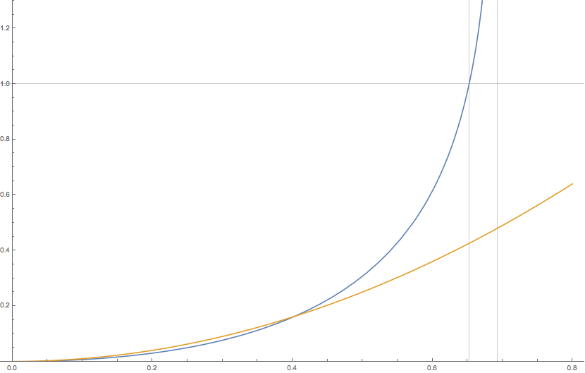
Numerically solving the above equation gives x0≈0.6524x_{0}\approx 0.6524, with the supremum in λ∗​(x0)\lambda^{*}(x_{0}) attained at β0=β∗​(x0)≈11.746\beta_{0}=\beta_{*}(x_{0})\approx 11.746. See Figure 2 for a comparison of the Gaussian rate function with λ∗\lambda^{*}, which is in some sense the “effective” rate function for XN​(t)X_{N}(t).

Refer to caption
Figure 2. Numerically generated plot of the rate function λ∗​(x)\lambda^{*}(x) from (1.7) (blue), with the Gaussian rate function x2x^{2} (orange) for comparison (normalized as in the upper tail N−x2+o⁡(1)N^{-x^{2}+o(1)} for the CUE field XN{CUE}​(t)X_{N}^{\cue}(t)). Included are the vertical lines x=x0=(λ∗)−1​(1)≈0.652x=x_{0}=(\lambda^{*})^{-1}(1)\approx 0.652, and x=log⁡2x=\log 2, where λ∗\lambda^{*} diverges. The lighter tail for XN​(t)X_{N}(t) as compared to that of the CUE helps explain the smaller value for the maximum.

We briefly indicate the way in which the function λ\lambda and the constant x0x_{0} arise in the proof of Theorem 1.2. Roughly speaking, we will model the field XN​(t)X_{N}(t) by a sequence (Y~​(t))t∈TN(\widetilde{Y}(t))_{t\in T_{N}} of weakly correlated variables indexed by a discrete set TNT_{N} of roughly NN equally spaced points tt in ℝ/ℤ{\mathbb{R}/\mathbb{Z}}. For each t∈TNt\in T_{N}, Y~​(t)\widetilde{Y}(t) is a sum of roughly log⁡N\log N i.i.d. copies of the variable VV in (1.4). (Such an approximation of XN​(t)X_{N}(t) can only be justified for points t∈ℝ/ℤt\in{\mathbb{R}/\mathbb{Z}} obeying a quantitative “minor arc” condition similar in spirit to the finite type condition (1.2).) Assuming the variables {Y~​(t)}t∈TN\{\widetilde{Y}(t)\}_{t\in T_{N}} are sufficiently weakly correlated, one can show that maxt∈TN⁡Y~​(t)=(x0+o⁡(1))​log⁡N\max_{t\in T_{N}}\widetilde{Y}(t)=(x_{0}+o(1))\log N with high probability. Indeed, the expected number of points t∈TNt\in T_{N} for which Y~​(t)≥x​log⁡N\widetilde{Y}(t)\geq x\log N is

|TN|​e−(λ∗​(x)+o⁡(1))​log⁡N=N1−λ∗​(x)+o⁡(1),|T_{N}|e^{-(\lambda^{*}(x)+o(1))\log N}=N^{1-\lambda^{*}(x)+o(1)},

which is o⁡(1)o(1) for x≥x0+ϵx\geq x_{0}+\epsilon. This leads to an upper bound on the maximum of Y~​(t)\widetilde{Y}(t) by Markov’s inequality. The lower bound is more involved and requires understanding the two-point correlations for the field XNX_{N}, which decay logarithmically with respect to a certain “arithmetic” distance.

A more detailed overview of proof ideas is provided in Section 2.

1.1. Organization of the paper

The rest of the paper is organized as follows. After setting up notation in Section 1.2, we give a high-level description of the main ideas of the proof in Section 2. In Section 3 we prove some preliminary estimates: Section 3.1 gives estimates on the distribution of cycle lengths for a random permuation, while Sections 3.2 and 3.3 provide lemmas that are used in Section 4 to estimate Fourier–Laplace transforms of the Poisson field. In Section 4 we also provide upper and lower bounds on large deviation events for the Poisson field (at one and two points). In Section 5 we prove the upper bound in Theorem 1.2, and we prove the matching lower bound in Sections 6 and 7.

1.2. Notation

We use the Vinogradov symbol ≪\ll; thus, f≪gf\ll g, g≫fg\gg f, f=O⁡(g)f=O(g) all mean |f|≤C​g|f|\leq Cg for some universal constant C<∞C<\infty. f≍gf\asymp g means f≪g≪ff\ll g\ll f. We indicate dependence of the implied constant on parameters with subscripts, e.g. f≪αgf\ll_{\alpha}g. f=oα;q→q0​(g)f=o_{\alpha;\,q\to q_{0}}(g) means that f/g→0f/g\to 0 as q→q0q\to q_{0} for any fixed value of the parameter α\alpha (so the rate of convergence may depend on α\alpha). In the usual case that the asymptotic parameter is NN we suppress the subscript N→∞N\to\infty: thus, f=o⁡(g)f=o(g), f=oα​(g)f=o_{\alpha}(g) mean f=oN→∞​(g)f=o_{N\to\infty}(g), f=oα;N→∞​(g)f=o_{\alpha;\,N\to\infty}(g). f=ω⁡(g)f=\omega(g) means g=o⁡(f)g=o(f).

For x∈ℝ/ℤx\in{\mathbb{R}/\mathbb{Z}}, ‖x‖ℝ/ℤ\|x\|_{\mathbb{R}/\mathbb{Z}} denotes the distance from xx to zero.

We use |S||S| to denote the cardinality of a set SS, and Leb⁡(E)\Leb(E) to denote the Lebesgue measure of a Borel set E⊂𝕋E\subset\mathbb{T}.

For an interval J⊂ℝJ\subset\mathbb{R}, by ∑j∈J\sum_{j\in J} we mean ∑j∈J∩ℤ\sum_{j\in J\cap\mathbb{Z}}. Sums written ∑j≤M\sum_{j\leq M} are understood to mean ∑1≤j≤M\sum_{1\leq j\leq M}.

We denote the Fourier coefficients of a function f:(ℝ/ℤ)d→ℂf:({\mathbb{R}/\mathbb{Z}})^{d}\to\mathbb{C} by

(1.10) f^(𝝃)=∫ℝ/ℤe(−𝝃⋅𝒕)f(𝒕)dt1⋯dtd,𝝃∈ℤd.\widehat{f}(\bm{\xi})=\int_{\mathbb{R}/\mathbb{Z}}e(-\bm{\xi}\cdot\bm{t})f(\bm{t})dt_{1}\cdots dt_{d},\quad\bm{\xi}\in\mathbb{Z}^{d}.

2. Proof overview

In this section we provide a high-level overview of proof ideas.

2.1. Decomposition of XNX_{N} into modes according to cycle structure

A routine computation shows that if QQ is the ℓ×ℓ\ell\times\ell permutation matrix for a cycle of length ℓ\ell, then

(2.1) det(1−z​Q)=1−zℓ.\det(1-zQ)=1-z^{\ell}.

Thus, letting Cℓ​(PN)C_{\ell}(P_{N}) denote the number of cycles of length ℓ\ell in the cycle decomposition of PNP_{N}, we have

(2.2) XN​(t)=∑ℓ=1NCℓ​(PN)​log⁡|1−e⁡(ℓ​t)|.X_{N}(t)=\sum_{\ell=1}^{N}C_{\ell}(P_{N})\log|1-e(\ell t)|.

Before proceeding we make a couple of quick observations. Since log⁡|1−e⁡(⋅)|\log|1-e(\cdot)| is uniformly bounded by log⁡2\log 2 on ℝ/ℤ{\mathbb{R}/\mathbb{Z}}, we have

(2.3) supt∈ℝ/ℤXN​(t)≤(log⁡2)​∑ℓ=1NCℓ​(PN) almost surely.\sup_{t\in{\mathbb{R}/\mathbb{Z}}}X_{N}(t)\leq(\log 2)\sum_{\ell=1}^{N}C_{\ell}(P_{N})\qquad\text{ almost surely.}

Moreover, an easy first and second moment argument for the total number of cycles (similar to the proof of Lemma 5.3 below) yields

(2.4) supt∈ℝ/ℤXN​(t)≤(log⁡2+ϵ)​log⁡N with probability 1−o⁡(1)\sup_{t\in{\mathbb{R}/\mathbb{Z}}}X_{N}(t)\leq(\log 2+\epsilon)\log N\qquad\text{ with probability $1-o(1)$}

for any fixed ϵ>0\epsilon>0. Since log⁡2≈0.693\log 2\approx 0.693, this fails to achieve the sharp bound of Theorem 1.2. However, we point out here that the same argument does achieve the sharp bound for the supremum of the imaginary part of log⁡χN​(e​(t))\log\chi_{N}(e(t)). Indeed, similarly to (2.2) we have

(2.5) Im​log​det(IN−e⁡(t)​PN)=∑ℓ=1NCℓ​(PN)​arg⁡(1−e⁡(ℓ​t)),\mathrm{Im}\,\log\det(I_{N}-e(t)P_{N})=\sum_{\ell=1}^{N}C_{\ell}(P_{N})\arg(1-e(\ell t)),

where we take the principal branch of arg\arg so that arg(1−e(u))∈[−π/2,π/2)\arg(1-e(u))\in[-\pi/2,\pi/2) for u∈ℝ/ℤu\in{\mathbb{R}/\mathbb{Z}}. Now we can bound

supt∈ℝ/ℤIm​log​det(IN−e⁡(t)​PN)≤π2​∑ℓ=1NCℓ​(PN)≤(π2+ϵ)​log​Nwith probability 1−o⁡(1).\sup_{t\in{\mathbb{R}/\mathbb{Z}}}\mathrm{Im}\,\log\det(I_{N}-e(t)P_{N})\leq\frac{\pi}{2}\sum_{\ell=1}^{N}C_{\ell}(P_{N})\leq\Big(\frac{\pi}{2}+\epsilon\Big)\log N\qquad\text{with probability $1-o(1)$.}

Conversely, one notes that for t∈(1−ϵ/N,1)t\in(1-\epsilon/N,1) we have arg⁡(1−e⁡(ℓ​t))>π2​(1−ϵ)\arg(1-e(\ell t))>\frac{\pi}{2}(1-\epsilon) for all 1≤ℓ≤N1\leq\ell\leq N, so in fact

supt∈ℝ/ℤIm​log​det(IN−e⁡(t)​PN)=(π2+o⁡(1))​log​Nwith probability 1−o⁡(1).\sup_{t\in{\mathbb{R}/\mathbb{Z}}}\mathrm{Im}\,\log\det(I_{N}-e(t)P_{N})=\Big(\frac{\pi}{2}+o(1)\Big)\log N\qquad\text{with probability $1-o(1)$.}

The reason the trivial upper bound for the imaginary part is sharp is that the function arg⁡(1−e⁡(u))=π⁡(u−12)\arg(1-e(u))=\pi(u-\frac{1}{2}) achieves its maximum in a neighborhood of zero, and for points tt very close to zero, the sequence (ℓ​t)ℓ∈[N](\ell t)_{\ell\in[N]} stays within such a neighborhood. By contrast, the function log⁡|1−e⁡(u)|\log|1-e(u)| diverges to −∞-\infty near zero, while the maximum is achieved at 1/21/2. This makes the upper bound (2.4) impossible to achieve (any sequence (ℓ​t)ℓ∈[N](\ell t)_{\ell\in[N]} visiting a neighborhood of 1/21/2 very often will also visit a neighborhood of zero very often). Instead, as we will see below, the maximum tends to be attained at “minor arc” points tt, for which the sequence (ℓ​t)ℓ∈[N](\ell t)_{\ell\in[N]} mixes rapidly in the torus, or equivalently, does not visit a small neighborhood of zero very often.

2.2. Poisson approximation

It is well known that for any fixed k∈ℕk\in\mathbb{N}, as N→∞N\to\infty the joint distribution of the cycle counts (C1​(PN),…,Ck​(PN))(C_{1}(P_{N}),\dots,C_{k}(P_{N})) converges in distribution to a sequence of independent Poisson variables (Z1,…,Zk)(Z_{1},\dots,Z_{k}), where 𝔼⁡Zℓ=1/ℓ\e Z_{\ell}=1/\ell. In fact, this still holds if kk grows with NN at any speed with k=o⁡(N)k=o(N), as shown by the following result of Arratia and Tavaré.

Theorem 2.1 (Poisson approximation [AT92, Theorem 2]).

Let (Zℓ)ℓ∈ℕ(Z_{\ell})_{\ell\in\mathbb{N}} denote a sequence of independent Poisson random variables with 𝔼⁡Zℓ=1/ℓ\e Z_{\ell}=1/\ell for each ℓ∈ℕ\ell\in\mathbb{N}. Let 1≤M≤N1\leq M\leq N. Then then following bound on the total variation distance between the sequences (Cℓ​(PN))ℓ≤M(C_{\ell}(P_{N}))_{\ell\leq M} and (Zℓ)ℓ≤M(Z_{\ell})_{\ell\leq M} holds:

supA∈ℤ≥0M|ℙ⁡((Cℓ​(PN))ℓ≤M∈A)−ℙ⁡((Zℓ)ℓ≤M∈A)|≤exp⁡(−(1+o⁡(1))​NM​log​NM​).\sup_{A\in\mathbb{Z}_{\geq 0}^{M}}\Big|\pr\Big((C_{\ell}(P_{N}))_{\ell\leq M}\in A\Big)-\pr\Big((Z_{\ell})_{\ell\leq M}\in A\Big)\Big|\leq\exp\left(-(1+o(1))\frac{N}{M}\log\frac{N}{M}\rule{0.0pt}{8.53581pt}\right).

See [AT92] for a more specific bound; for us it is only important that the total variation distance goes to zero if M=o⁡(N)M=o(N).

This motivates splitting the permutation field XNX_{N} as follows. We first truncate the sum in (2.2). Let WW be a sowly growing parameter satisfying

(2.6) ω⁡(1)≤W≤No⁡(1)\omega(1)\leq W\leq N^{o(1)}

and write

(2.7) XN​(t)\displaystyle X_{N}(t) =∑ℓ≤N/WCℓ​(PN)​log⁡|1−e⁡(ℓ​t)|+∑N/W<ℓ≤NCℓ​(PN)​log|1−e⁡(ℓ​t)|=:XN≤​(t)+XN>​(t).\displaystyle=\sum_{\ell\leq N/W}C_{\ell}(P_{N})\log|1-e(\ell t)|+\sum_{N/W<\ell\leq N}C_{\ell}(P_{N})\log|1-e(\ell t)|=:X_{N}^{\leq}(t)+X_{N}^{>}(t).

Let (Zℓ)ℓ≥1(Z_{\ell})_{\ell\geq 1} be a sequence of independent Poisson variables with 𝔼⁡Zℓ=1/ℓ\e Z_{\ell}=1/\ell, and define the Poisson field

(2.8) YN​(t)=∑ℓ≤NZℓ​log⁡|1−e⁡(ℓ​t)|.Y_{N}(t)=\sum_{\ell\leq N}Z_{\ell}\log|1-e(\ell t)|.

From Theorem 2.1, we can understand the maximum of the field XN≤X_{N}^{\leq} by instead considering the Poisson field YN/WY_{N/W}. Then we have two problems:

  1. (I)

    Estimate the maximum of YN/W​(t)Y_{N/W}(t).

  2. (II)

    Show that the high frequency tail XN>X_{N}^{>} has negligible impact.

2.3. Upper bound: Failure of the first moment method

We begin the discussion of how to prove the upper bound in Theorem 1.2, i.e. that for any fixed ϵ∈(0,1)\epsilon\in(0,1),

(2.9) supt∈ℝ/ℤXN​(t)≤(x0+ϵ)​log⁡N with probability 1−oϵ​(1).\sup_{t\in{\mathbb{R}/\mathbb{Z}}}X_{N}(t)\leq(x_{0}+\epsilon)\log N\qquad\text{ with probability $1-o_{\epsilon}(1)$}.

For the upper bound, problem (II) is relatively simple: a straightforward second moment computation shows that with probability 1−o⁡(1)1-o(1),

(2.10) maxt∈ℝ/ℤ⁡XN>​(t)≤O⁡(log⁡W)=o⁡(log⁡N);\max_{t\in{\mathbb{R}/\mathbb{Z}}}X_{N}^{>}(t)\leq O(\log W)=o(\log N)\,;

see Lemma 5.3. The key point is that the functions log|1−e(ℓ⋅)|\log|1-e(\ell\,\cdot)| are bounded pointwise by log⁡2<1\log 2<1 on ℝ/ℤ{\mathbb{R}/\mathbb{Z}}, so XN>​(t)X_{N}^{>}(t) is uniformly controlled by the number of cycles of length between N/WN/W and NN. (As we discuss below, problem (II) is significantly more challenging for proving the lower bound due to the singularities of log|1−e(ℓ⋅)|\log|1-e(\ell\,\cdot)|.) Thus, to prove (2.9) our task is reduced to showing the same estimate for the Poisson field YN/WY_{N/W}, which from (2.6) is equivalent to showing

(2.11) supt∈ℝ/ℤYN​(t)≤(x0+ϵ)​log⁡N with probability 1−oϵ​(1).\sup_{t\in{\mathbb{R}/\mathbb{Z}}}Y_{N}(t)\leq(x_{0}+\epsilon)\log N\qquad\text{ with probability $1-o_{\epsilon}(1)$}.

It turns out it is enough to control the maximum on a fine mesh for the torus. (Actually, in the proof it will be more convenient to pass to a mesh before replacing the permutation field XNX_{N} with the Poisson field YNY_{N}, but we ignore this point here.) Specifically, it will suffice to show

(2.12) maxt∈TN⁡YN​(t)≤(x0+ε)​log⁡Nwith probability ​1−o⁡(1)\max_{t\in T_{N}}Y_{N}(t)\leq(x_{0}+\varepsilon)\log N\qquad\text{with probability }1-o(1)

where TN⊂ℝ/ℤT_{N}\subset{\mathbb{R}/\mathbb{Z}} is a finite mesh for ℝ/ℤ{\mathbb{R}/\mathbb{Z}} of cardinality O⁡(N)O(N).

Following the standard first moment paradigm, see e.g. [ABB17] for a similar approach, we consider the super-level sets

(2.13) 𝒮NY​(T,x):={t∈T:YN​(t)≥x​log⁡N}\mathcal{S}^{Y}_{N}(T,x):=\{t\in T:Y_{N}(t)\geq x\log N\}

with T=TNT=T_{N}. From Markov’s inequality, for the upper bound in Theorem 1.2 it will suffice to establish the first moment estimate

(2.14) 𝔼⁡|𝒮NY​(T,x0+ϵ)|=∑t∈Tℙ⁡(YN​(t)≥(x0+ϵ)​log⁡N)=oϵ​(1).\e|\mathcal{S}^{Y}_{N}(T,x_{0}+\epsilon)|=\sum_{t\in T}\pr(Y_{N}(t)\geq(x_{0}+\epsilon)\log N)=o_{\epsilon}(1).

Our task thus reduces to a large deviations problem: to obtain accurate estimates for the tail events {YN(t)≥xlogN}\{Y_{N}(t)\geq x\log N\} at different points t∈ℝ/ℤt\in{\mathbb{R}/\mathbb{Z}}. (Recall that, in contrast to the CUE field discussed around (1.3), the distribution of YN​(t)Y_{N}(t) depends on tt.) As YN​(t)Y_{N}(t) is a sum of independent variables, we can obtain accurate upper bounds on tail events by Laplace’s method. We can easily evaluate the Laplace transform:

(2.15) 𝔼⁡eβ​YN​(t)=∏ℓ≤N𝔼⁡exp⁡(β​Zℓ​log⁡|1−e⁡(ℓ​t)|​)=exp⁡(∑ℓ≤N1ℓ​(|1−e⁡(ℓ​t)|β−1)).\e e^{\beta Y_{N}(t)}=\prod_{\ell\leq N}\e\exp\left(\beta Z_{\ell}\log|1-e(\ell t)|\rule{0.0pt}{8.53581pt}\right)=\exp\bigg(\sum_{\ell\leq N}\frac{1}{\ell}\left(|1-e(\ell t)|^{\beta}-1\right)\bigg).

From considerations of Diophantine approximation that will be discussed in Section 2.6, one can show that for generic points t∈ℝ/ℤt\in{\mathbb{R}/\mathbb{Z}} (points that are in a certain quantitative sense “sufficiently irrational”),

(2.16) log⁡𝔼⁡eβ​YN​(t)=∑ℓ≤N1ℓ​(|1−e⁡(ℓ​t)|β−1)=(∫ℝ/ℤ(|1−e⁡(u)|β−1)​du+o⁡(1))​log​N,\log\e e^{\beta Y_{N}(t)}=\sum_{\ell\leq N}\frac{1}{\ell}\left(|1-e(\ell t)|^{\beta}-1\right)=\bigg(\int_{\mathbb{R}/\mathbb{Z}}(|1-e(u)|^{\beta}-1)du+o(1)\bigg)\log N,

where, crucially, the error o⁡(1)o(1) is uniform over all generic points tt. Applying Markov’s inequality to an exponential moment 𝔼⁡exp⁡(β​YN​(t))\e\exp(\beta Y_{N}(t)) and optimizing β\beta one obtains a sharp upper tail bound for YN​(t)Y_{N}(t) at such points. Assuming (optimistically) that our mesh TNT_{N} contains only generic points, then upon inserting the resulting tail bounds into (2.14), a computation shows

𝔼⁡|𝒮NY​(T,x)|≍{N−c⁡(ε)for ​x=1+εNc′​(ε)for ​x=1−ε\e|\mathcal{S}^{Y}_{N}(T,x)|\asymp\begin{cases}N^{-c(\varepsilon)}&\text{for }x=1+\varepsilon\\ N^{c^{\prime}(\varepsilon)}&\text{for }x=1-\varepsilon\end{cases}

for any sufficiently small ε>0\varepsilon>0, where c⁡(ε),c′​(ε)c(\varepsilon),c^{\prime}(\varepsilon) are positive constants depending only on ε\varepsilon. In particular, this first moment computation suggests (incorrectly) that x0=1x_{0}=1. From Markov’s inequality we obtain the upper bound

(2.17) maxt∈TN⁡YN​(t)≤(1+ε)​log⁡Nwith probability ​1−oϵ​(1).\max_{t\in T_{N}}Y_{N}(t)\leq(1+\varepsilon)\log N\qquad\text{with probability }1-o_{\epsilon}(1).

Recalling that x0≈0.652x_{0}\approx 0.652, this bound is consistent with (2.12) but not sharp – in fact, it even fails to beat the trivial bound (2.4).

2.4. Conditioning on a typical distribution of cycle lengths at coarse scale

To obtain the sharp bound in Theorem 1.2 we need to modify our first and second moment computations to avoid a certain class of rare events. Indeed, there is a class of small events on which the maximum of YN​(t)Y_{N}(t) is atypically large (of size ∼x​log⁡N\sim x\log N for some x∈(x0,1)x\in(x_{0},1)), but which are of probability N−cN^{-c} for some c∈(0,1)c\in(0,1). When we are looking at height xx these events cause the first moment to blow up. However, the first moment (i.e. the union bound) is wasteful as these events have significant overlap for different values of t∈ℝ/ℤt\in{\mathbb{R}/\mathbb{Z}}.

Roughly speaking, the problematic events occur when there is a “clump” in the sequence of Poisson variables ZℓZ_{\ell} (or cycle counts Cℓ​(PN)C_{\ell}(P_{N})) – specifically, when 𝒩⁡(I):=∑ℓ∈IZℓ\mathcal{N}(I):=\sum_{\ell\in I}Z_{\ell} is atypically large for a short interval II. Recall that 𝔼⁡Zℓ=1/ℓ\e Z_{\ell}=1/\ell, so “large” and “short” in the preceding sentence depend on the position of ℓ∈[N]\ell\in[N] (for instance when ℓ\ell is of order NN the event that 𝒩⁡({ℓ})=Zℓ≥2\mathcal{N}(\{\ell\})=Z_{\ell}\geq 2 is atypical). Since 𝔼∑ℓ≤NZℓ=logN+O(1)\e\sum_{\ell\leq N}Z_{\ell}=\log N+O(1), we expect gaps between consecutive nonzero variables ZℓZ_{\ell} to be of order ℓ\ell. Thus, for a given expected size for 𝒩⁡(I)\mathcal{N}(I) we should consider intervals of exponentially growing length. If it occurs that a large number of cycles have lengths in the interval [ℓ,(1+δ)​ℓ][\ell,(1+\delta)\ell] for some ℓ∼Nc\ell\sim N^{c} and small δ>0\delta>0, then the corresponding modes t↦log⁡|1−(ℓ​t)|t\mapsto\log|1-(\ell t)| in the expansion (2.2) (or (2.8)) will add constructively on large subsets of ℝ/ℤ{\mathbb{R}/\mathbb{Z}} (roughly, on intervals of length ∼N−c\sim N^{-c} spaced at distance ∼1/δ\sim 1/\delta from each other), creating an atypically large number of high points (on the order of δ​N1−c\delta N^{1-c}).

We deal with these rare clumping events by grouping the summands in (2.8) into intervals with a lacunary sequence of endpoints, and conditioning on the event that (for most intervals) there is at most one nonzero summand. To state this more precisely we develop some additional notation. For J⊂ℝ+J\subset\mathbb{R}_{+} we let

(2.18) 𝒩⁡(J)=∑ℓ∈J∩ℤZℓ\mathcal{N}(J)=\sum_{\ell\in J\cap\mathbb{Z}}Z_{\ell}

denote the number of “cycles” with lengths in the set JJ (recall the ZℓZ_{\ell} are actually Poisson variables that model the cycle counts), and for t∈ℝ/ℤt\in{\mathbb{R}/\mathbb{Z}} we write

(2.19) YJ​(t)=∑ℓ∈J∩ℤZℓ​log⁡|1−e⁡(ℓ​t)|Y_{J}(t)=\sum_{\ell\in J\cap\mathbb{Z}}Z_{\ell}\log|1-e(\ell t)|

for the contribution of these cycles to the field YN​(t)Y_{N}(t) (assuming J⊂(0,N]J\subset(0,N]). We let ϱ∈(0,1/2)\varrho\in(0,1/2) be a small parameter (which may depend on NN and ϵ\epsilon) and for k≥0{k}\geq 0 denote

(2.20) Ik=[eϱ​k,eϱ⁡(k+1)),ρk=𝔼⁡𝒩⁡(Ik)=∑ℓ∈Ik1ℓ.I_{k}=[e^{\varrho{k}},e^{\varrho({k}+1)}),\qquad\rho_{k}=\e\mathcal{N}(I_{k})=\sum_{\ell\in I_{k}}\frac{1}{\ell}.

Taking ϱ,n\varrho,n depending on N,ϵN,\epsilon is such a way that

(2.21) ϱ​n=(1+o⁡(1))​log⁡N\varrho n=(1+o(1))\log N

it now suffices to show

(2.22) maxt∈TN⁡Y[1,eϱ​n)​(t)=max⁡∑1≤k<nt∈TN⁡YIk​(t)≤(1+ϵ)​ϱ​n with probability 1−oϵ​(1).\max_{t\in T_{N}}Y_{[1,e^{\varrho n})}(t)=\max_{t\in T_{N}}\sum_{1\leq{k}<n}Y_{I_{k}}(t)\leq(1+\epsilon)\varrho n\qquad\text{ with probability $1-o_{\epsilon}(1)$}.

The variables 𝒩⁡(Ik)\mathcal{N}(I_{k}) are independent Poisson variables with expectation ρk\rho_{k}, and for k{k} reasonably large we have ρk≈ϱ\rho_{k}\approx\varrho (specifically, if k=ω⁡(1ϱ​log⁡1ϱ){k}=\omega(\frac{1}{\varrho}\log\frac{1}{\varrho}) then ρk=(1+o⁡(1))​ϱ\rho_{k}=(1+o(1))\varrho). To avoid the atypical clumping events described above we will condition on a “typical” sequence of the partial sums 𝒩⁡(Ik)\mathcal{N}(I_{k}). For a≥0a\geq 0 let

(2.23) Qa={k≥0:𝒩⁡(Ik)=a},Q≥a={k≥0:𝒩⁡(Ik)≥a}Q_{a}=\{{k}\geq 0:\mathcal{N}(I_{k})=a\},\qquad Q_{\geq a}=\{{k}\geq 0:\mathcal{N}(I_{k})\geq a\}

denote the sets k{k} indexing intervals IkI_{k} containing exactly aa cycles and at least aa cycles, respectively. When ϱ\varrho is sufficiently small, for a long interval [m,n)[m,n) we expect (roughly speaking)

(2.24) |Q0∩[m,n)|≈(1−ϱ)​(n−m),|Q1∩[m,n)|≈ϱ⁡(n−m),|Q≥2∩[m,n)|≈0.|Q_{0}\cap[m,n)|\approx(1-\varrho)(n-m),\qquad|Q_{1}\cap[m,n)|\approx\varrho(n-m),\qquad|Q_{\geq 2}\cap[m,n)|\approx 0.

We will condition on fixed realizations Q,Q~Q,\widetilde{Q} for Q1∩[m,n)Q_{1}\cap[m,n) and Q≥2∩[m,n)Q_{\geq 2}\cap[m,n), respectively, satisfying the above. For given m,n,Q,Q~m,n,Q,\widetilde{Q} we denote the event

(2.25) 𝒬:=𝒬(m,n,Q,Q~):={Q1∩[m,n)=Q,Q≥2∩[m,n)=Q~}.\mathcal{Q}:=\mathcal{Q}(m,n,Q,\widetilde{Q}):=\left\{Q_{1}\cap[m,n)=Q,\quad Q_{\geq 2}\cap[m,n)=\widetilde{Q}\right\}.

With a fixed choice of m,n,Q,Q~m,n,Q,\widetilde{Q} we will often abbreviate

(2.26) 𝔼𝒬(⋅):=𝔼(⋅|𝒬),ℙ𝒬(⋅):=𝔼𝒬𝟙(⋅).\e^{\mathcal{Q}}(\,\cdot\,):=\e\left(\,\cdot\ \middle|\ \mathcal{Q}\right),\qquad\pr^{\mathcal{Q}}(\,\cdot\,):=\e^{\mathcal{Q}}\ind(\,\cdot\,).

Now in place of (2.14) we want to show that for a typical choice of Q,Q~Q,\widetilde{Q},

(2.27) 𝔼𝒬⁡|𝒮⌊eϱ​n⌋Y​(T,x0+ϵ)|=∑t∈Tℙ𝒬⁡(Y[1,eϱ​n)​(t)≥(x0+ϵ)​ϱ​n)=oϵ​(1).\e^{\mathcal{Q}}|\mathcal{S}^{Y}_{\lfloor e^{\varrho n}\rfloor}(T,x_{0}+\epsilon)|=\sum_{t\in T}\pr^{\mathcal{Q}}\Big(Y_{[1,e^{\varrho n})}(t)\geq(x_{0}+\epsilon)\varrho n\Big)=o_{\epsilon}(1).

(2.22) then follows from Markov’s inequality and the fact that we conditioned on typical realizations of Q1,Q≥2Q_{1},Q_{\geq 2}.

Note that (2.24) suggests that for typical choices of Q,Q~Q,\widetilde{Q}, on the event 𝒬⁡(1,n,Q,Q~)\mathcal{Q}(1,n,Q,\widetilde{Q}),

Y[1,eϱ​n)​(t)≈∑k∈QYIk​(t),Y_{[1,e^{\varrho n})}(t)\approx\sum_{{k}\in Q}Y_{I_{k}}(t),

where for k∈Qk\in Q,

YIk​(t)=log⁡|1−e⁡(ℓk​t)|Y_{I_{k}}(t)=\log|1-e(\bm{\ell}_{k}t)|

and ℓk\bm{\ell}_{k} is a random element of IkI_{k} with distribution ℙ⁡(ℓk=ℓ)∝1ℓ​1ℓ∈Ik\pr(\bm{\ell}_{k}=\ell)\propto\frac{1}{\ell}1_{\ell\in I_{k}}. As will be discussed below, in the generic case that t∈ℝ/ℤt\in{\mathbb{R}/\mathbb{Z}} is not too close to a rational with small denominator, the sequence {ℓ​t}ℓ∈Ik⊂ℝ/ℤ\{\ell t\}_{\ell\in I_{k}}\subset{\mathbb{R}/\mathbb{Z}} rapidly equidistributes in the torus. One can use this together with (1.5) to show that for such points tt and for k∈Q{k}\in Q,

𝔼𝒬⁡YIk​(t)=𝔼⁡(YIk​(t)|𝒩⁡(Ik)=1)≈0.\e^{\mathcal{Q}}Y_{I_{k}}(t)=\e\left(Y_{I_{k}}(t)\,\big|\,\mathcal{N}(I_{k})=1\right)\approx 0.

One can similarly show that at such points tt the variables {YIk​(t)}k∈Q\{Y_{I_{k}}(t)\}_{{k}\in Q} have comparable variance. Thus we expect the variables YIk​(t)Y_{I_{k}}(t) to have comparable contribution to the fluctuations of Y[1,eϱ​n)​(t)Y_{[1,e^{\varrho n})}(t) (at least for generic points t∈ℝ/ℤt\in{\mathbb{R}/\mathbb{Z}}).

2.5. Upper bound: major and minor arcs

To show (2.27) we need accurate estimates on the summands; the value for x0x_{0} will then be the critical value of xx at which the tail probability

(2.28) ℙ𝒬⁡(Y[1,eϱ​n)​(t)≥x​ϱ​n)\pr^{\mathcal{Q}}\Big(Y_{[1,e^{\varrho n})}(t)\geq x\varrho n\Big)

is of order e−ϱ​n+o⁡(1)=N−1+o⁡(1)e^{-\varrho n+o(1)}=N^{-1+o(1)}, balancing the entropy cost |T|≍N|T|\asymp N.

A major difficulty is that the distribution of YN​(t)Y_{N}(t), and in particular the tail probabilities (2.28), depend on the choice of t∈ℝ/ℤt\in{\mathbb{R}/\mathbb{Z}}. Indeed, a moment’s thought reveals there is no hope of showing a probability estimate of size e−ϱ​n+o⁡(1)e^{-\varrho n+o(1)} for all tt: consider for instance taking t=0t=0, where YNY_{N} (and XNX_{N}) are −∞-\infty for all NN. Moreover, for any rational p/q∈ℝ/ℤp/q\in{\mathbb{R}/\mathbb{Z}} with q=O⁡(1)q=O(1) we have that ℙ⁡(Zq≠0)\pr(Z_{q}\neq 0) is of constant order, and from (2.8) we see that YN​(p/q)=−∞Y_{N}(p/q)=-\infty on this event.

One thus sees that a general obstruction to obtaining nice tail estimates for YN​(t)Y_{N}(t) is that tt is well-approximated by a rational with small denominator. We quantify this in terms of Bohr sets. Recall that for an integer frequency ξ∈ℤ\xi\in\mathbb{Z} and κ∈(0,1)\kappa\in(0,1), the associated Bohr set is defined

(2.29) Bξ​(κ)={t∈ℝ/ℤ:‖ξ​t‖ℝ/ℤ≤κ}B_{\xi}(\kappa)=\{t\in{\mathbb{R}/\mathbb{Z}}:\|\xi t\|_{\mathbb{R}/\mathbb{Z}}\leq\kappa\}

(recall our notation ‖s‖ℝ/ℤ\|s\|_{\mathbb{R}/\mathbb{Z}} for the distance from ss to 0 in the torus). For a cuttoff frequency ξ0∈ℕ\xi_{0}\in\mathbb{N} we denote the set of “major arc points”

(2.30) Maj⁡(ξ0,κ)=⋃1≤ξ≤ξ0Bξ​(κ).\Maj(\xi_{0},\kappa)=\bigcup_{1\leq\xi\leq\xi_{0}}B_{\xi}(\kappa).

Borrowing terms from the Hardy–Littlewood circle method, we refer to elements of the complement ℝ/ℤ∖Maj⁡(ξ0,κ){\mathbb{R}/\mathbb{Z}}\setminus\Maj(\xi_{0},\kappa) as “minor arc points”. (Viewed as a subset of the circle ∂𝔻=e⁡(ℝ/ℤ)\partial\mathbb{D}=e({\mathbb{R}/\mathbb{Z}}), Maj⁡(ξ0,κ)\Maj(\xi_{0},\kappa) is a union of arcs with lengths in {2​κ/ξ:1≤ξ≤ξ0}\{2\kappa/\xi:1\leq\xi\leq\xi_{0}\}.) We will take ξ0,κ\xi_{0},\kappa small enough that Maj⁡(ξ0,κ)\Maj(\xi_{0},\kappa) has Lebesgue measure o⁡(1)o(1), so that generic points in the torus are minor arc.

For major arc points tt the sequence {ℓ​t}ℓ≥1⊂ℝ/ℤ\{\ell t\}_{\ell\geq 1}\subset{\mathbb{R}/\mathbb{Z}} is poorly mixing, and for small values of ℓ\ell it returns often to a small neighorhood of 00. Since log⁡|1−e⁡(⋅)|\log|1-e(\,\cdot\,)| is very negative there, from (2.8) one can (correctly) guess it is possible to choose ξ0,κ\xi_{0},\kappa in such a way that, with high probability, the values of ℓ\ell corresponding to these visits cause a large deficit in the value of YN​(t)Y_{N}(t) that cannot be compensated by all of the other terms in the sum. Thus, with high probability, the Poisson field does not even take positive values at major arc points, and it only remains to establish (2.22) with the supremum restricted to minor arcs.

While major arcs were fairly easy to handle in the proof of the upper bound, they will enter the proof of the lower bound in a more subtle way, as will be discussed in Section 2.7.

2.6. Large deviation estimates for the field on minor arcs

For t∈ℝ/ℤt\in{\mathbb{R}/\mathbb{Z}} that are minor arc we can obtain fairly accurate estimates on the tails of partial sums Y[eϱ​m,eϱ​n)​(t)Y_{[e^{\varrho m},e^{\varrho n})}(t), with uniform error bounds depending on ξ0,κ\xi_{0},\kappa. We briefly indicate why Bohr sets should play such a role. For the sake of discussion we ignore the contribution of cycles with lengths in Q~\widetilde{Q}. From large deviations theory we can deduce accurate tail estimates from estimates on the moment generating function

(2.31) 𝔼𝒬⁡exp⁡(β​∑k∈QYIk​(t))=∏k∈Qexp⁡(β​YIk​(t)|𝒩⁡(Ik)=1​)=∏k∈Q(1ρk​∑ℓ∈Ik|1−e⁡(ℓ​t)|βℓ)\e^{\mathcal{Q}}\exp\bigg(\beta\sum_{{k}\in Q}Y_{I_{k}}(t)\bigg)=\prod_{{k}\in Q}\exp\left(\beta Y_{I_{k}}(t)\,\middle|\,\mathcal{N}(I_{k})=1\rule{0.0pt}{8.53581pt}\right)=\prod_{{k}\in Q}\bigg(\frac{1}{\rho_{k}}\sum_{\ell\in I_{k}}\frac{|1-e(\ell t)|^{\beta}}{\ell}\bigg)

(compare with (2.16)). Recalling that ρk=∑ℓ∈Ik1/ℓ\rho_{k}=\sum_{\ell\in I_{k}}1/\ell, we recognize the above as a logarithmic average of the function ϕβ:=|1−e⁡(⋅)|β\phi_{\beta}:=|1-e(\,\cdot\,)|^{\beta} from ℝ/ℤ{\mathbb{R}/\mathbb{Z}} to ℝ\mathbb{R} along the Kronecker sequence {ℓ​t}m≤ℓ<n⊂ℝ/ℤ\{\ell t\}_{m\leq\ell<n}\subset{\mathbb{R}/\mathbb{Z}}. Now it is well known that that if t∈ℝ/ℤt\in{\mathbb{R}/\mathbb{Z}} is irrational and f:ℝ/ℤ→ℂf:{\mathbb{R}/\mathbb{Z}}\to\mathbb{C} is continuous, we have

1n​∑ℓ≤nf⁡(ℓ​t)⟶∫ℝ/ℤf⁡(u)​𝑑u as n→∞;\frac{1}{n}\sum_{\ell\leq n}f(\ell t)\longrightarrow\int_{\mathbb{R}/\mathbb{Z}}f(u)du\qquad\text{ as $n\to\infty$};

from summation by parts we get the same limit for the logarithmic averages 1log⁡n​∑ℓ≤nf⁡(ℓ​t)ℓ\frac{1}{\log n}\sum_{\ell\leq n}\frac{f(\ell t)}{\ell}. However, we require quantitative bounds depending on parameters ξ0,κ\xi_{0},\kappa, which we obtain in Section 3 by standard Fourier-analytic arguments. These estimates show

|1ρk​∑ℓ∈Ik|1−e⁡(ℓ​t)|βℓ−∫ℝ/ℤ|1−e⁡(u)|β​𝑑u|≤Error​(k,ϱ,ξ0,κ)\left|\frac{1}{\rho_{k}}\sum_{\ell\in I_{k}}\frac{|1-e(\ell t)|^{\beta}}{\ell}-\int_{\mathbb{R}/\mathbb{Z}}|1-e(u)|^{\beta}du\right|\leq\text{Error}({k},\varrho,\xi_{0},\kappa)

where the right hand side is ok→∞​(1)o_{{k}\to\infty}(1) for ϱ\varrho sufficiently small and appropriate choices of ξ0,κ\xi_{0},\kappa. From the above and (2.31), and recalling (1.6), we can show

(2.32) 𝔼𝒬⁡exp⁡(β​∑k∈QYIk​(t))=(1+on−m→∞​(1))​eλ⁡(β)​|Q|\e^{\mathcal{Q}}\exp\bigg(\beta\sum_{{k}\in Q}Y_{I_{k}}(t)\bigg)=(1+o_{n-m\to\infty}(1))e^{\lambda(\beta)|Q|}

for appropriate ξ0,κ\xi_{0},\kappa depending on n,mn,m (see Proposition 4.3 for a precise statement).

The above estimate suggests comparing Y[eϱ​m,eϱ​n)​(t)Y_{[e^{\varrho m},e^{\varrho n})}(t) with a sum of i.i.d. copies of the variable VV from (1.4). Let (Uk)k∈Q(U_{k})_{{k}\in Q} be a sequence of i.i.d. uniform elements of ℝ/ℤ{\mathbb{R}/\mathbb{Z}} and put

(2.33) Vk=log⁡|1−e⁡(Uk)|,Y~Q=∑k∈QVk.V_{k}=\log|1-e(U_{k})|,\qquad\widetilde{Y}_{Q}=\sum_{{k}\in Q}V_{k}.

We recognize the main term on the right hand side of (2.32) as the moment generating function for Y~Q\widetilde{Y}_{Q}. We can use this estimate to make a comparison of the form

(2.34) ℙ𝒬⁡(Y[eϱ​m,eϱ​n)​(t)≥y​|Q|)=(1+o⁡(1))​ℙ⁡(Y~Q≥y​|Q|)\pr^{\mathcal{Q}}\big(Y_{[e^{\varrho m},e^{\varrho n})}(t)\geq y|Q|\big)=(1+o(1))\pr\big(\widetilde{Y}_{Q}\geq y|Q|\big)

(see Proposition 4.6 for the quantitative estimate). This comparison yields a tail bound that is sufficient to complete the proof of (2.22) for minor arc points, and hence the upper bound in Theorem 1.2 (in fact we can even get by with a weaker tail estimate given by Corollary 4.2). Note the comparison (2.34) and the form of the moment generating function for Y~Q\widetilde{Y}_{Q} explain where the definition of the constant x0x_{0} in (1.9) comes from.

For the proof of the lower bound by a second moment argument we will also need joint tail estimates for partial sums of the Poisson field at two points s,t∈ℝ/ℤs,t\in{\mathbb{R}/\mathbb{Z}}. We defer discussion of this to the following subsection.

2.7. Lower bound: Logarithmic decay of correlations and structural dichotomy for high points

On a conceptual level we find it convenient to adopt some terminology that is suggestive of analogies with branching processes. For M≤NM\leq N, let us denote the partially summed field

(2.35) X≤M​(t)=∑ℓ≤MCℓ​(PN)​log⁡|1−e⁡(ℓ​t)|,X_{\leq M}(t)=\sum_{\ell\leq M}C_{\ell}(P_{N})\log|1-e(\ell t)|,

and for a level x∈ℝx\in\mathbb{R}, the associated set of “survivors”

(2.36) 𝒮≤M​(x)={t∈TN:X≤M​(t)≥x​log⁡M},\mathcal{S}_{\leq M}(x)=\{t\in T_{N}:X_{\leq M}(t)\geq x\log M\},

where, as before, TNT_{N} is a fixed mesh for ℝ/ℤ{\mathbb{R}/\mathbb{Z}} of size O⁡(N)O(N). (We will need to take TNT_{N} to be a slight rotation of the set of N′N^{\prime}-th roots of unity for some N′=O⁡(N)N^{\prime}=O(N), but we do not discuss this issue here.) We think of the cutoff MM as a time parameter, and 𝒮≤M​(x)\mathcal{S}_{\leq M}(x) as the portion of an initial “population” TNT_{N} that has attained a “fitness level” xx.

Our goal is to show that the final set of survivors 𝒮≤N​(x0−ϵ)\mathcal{S}_{\leq N}(x_{0}-\epsilon) is non-empty with high probability. This task is considerably more delicate than for the upper bound. We track the population across three epochs:

  1. (1)

    (Early generations): We show

    (2.37) 𝒮≤Nc​(−C)≫N with high probability\mathcal{S}_{\leq N^{c}}(-C)\gg N\qquad\text{ with high probability}

    for some constants C,c>0C,c>0 sufficiently large and small, respectively.

  2. (2)

    (Middle generations): Letting WW be a slowly growing parameter as in (2.6), we show

    (2.38) |𝒮≤N/W​(x0−ϵ)|≥Nc⁡(ϵ) with high probability.|\mathcal{S}_{\leq N/W}(x_{0}-\epsilon)|\geq N^{c(\epsilon)}\qquad\text{ with high probability}.
  3. (3)

    (Late generations): Finally, we argue

    (2.39) |𝒮≤N​(x0−2​ϵ)|≥1 with high probability.|\mathcal{S}_{\leq N}(x_{0}-2\epsilon)|\geq 1\qquad\text{ with high probability.}

For early and middle generations we can use Theorem 2.1 to replace the cycle counts Cℓ​(PN)C_{\ell}(P_{N}) with Poisson variables ZℓZ_{\ell}, as we did for the upper bound. The reason to consider early generations separately is to gain some independence between different “lineages” for the second moment argument for middle generations. The basic idea for establishing (2.37) is that the partially summed Poisson field Y≤M​(t)=∑≤MZℓ​log⁡|1−e⁡(ℓ​t)|Y_{\leq M}(t)=\sum_{\leq M}Z_{\ell}\log|1-e(\ell t)| is an average over samples from the mean zero function log⁡|1−e⁡(⋅)|\log|1-e(\cdot)|; since we already have control on such random averages from above, we can argue that the truncated field can’t be too much smaller than its average value at too many points t∈ℝ/ℤt\in{\mathbb{R}/\mathbb{Z}}.

For the middle generations we adapt a well known second moment argument for the maximum of branching random walk, the basic ideas of which go back to [Bra78]. (The analogue of Theorem 1.2 for branching random walk goes back a bit further – see [Ham74, Theorem 2], as well as [Kin75, Kin76, Big77].) The second moment argument is also used in the works [ABB17, PZ17, CMN16] on the maximum for the CUE field. We will not review the detailed argument here, and instead refer the reader to [Arg17, Kis15, Zei16] for an exposition. The main point is that a straightforward application of the second moment method to the number of survivors |𝒮≤N/W​(x0−ϵ)||\mathcal{S}_{\leq N/W}(x_{0}-\epsilon)| fails to show it is nonzero with high probability, despite the fact that its first moment is of size Nc⁡(ϵ)N^{c(\epsilon)}. Instead, we compute the first and second moments of a (smaller) number of points t∈TNt\in T_{N} for which the partially summed Poisson field Y≤M​(t)Y_{\leq M}(t) makes steady progress towards the extreme level x0​log⁡Nx_{0}\log N. We measure the notion of steady progress, in terms advocated by Kistler [Kis15], as follows. Conditioning on an event 𝒬\mathcal{Q} as in (2.25), for integers n1<n2n_{1}<n_{2} we denote the partial lineage of a point t∈TNt\in T_{N}

(2.40) Δn1,n2​(t):=∑k∈Q∩[n1,n2)YIk​(t)=∑k∈Q∩[n1,n2)∑eϱ​n1≤ℓ<eϱ​n2Zℓ​log⁡|1−e⁡(ℓ​t)|.\Delta_{n_{1},n_{2}}(t):=\sum_{k\in Q\cap[n_{1},n_{2})}Y_{I_{k}}(t)=\sum_{k\in Q\cap[n_{1},n_{2})}\sum_{e^{\varrho n_{1}}\leq\ell<e^{\varrho n_{2}}}Z_{\ell}\log|1-e(\ell t)|.

For a large parameter KK (which we eventually take to be of size ≫1/ϵ\gg 1/\epsilon) we cut the set Q∩[1,n)Q\cap[1,n) into KK legs Qi=Q∩[(i−1)​n/K,i​n/K)Q_{i}=Q\cap[(i-1)n/K,in/K), and aim to show that the set of “rapidly rising” points

(2.41) ℛn​(TN,x0−ϵ)={t∈TN:Δ(i−1)​nK,i​nK​(t)≥(x0−ϵ)​|Qi|​∀2≤i≤K}\mathcal{R}_{n}(T_{N},x_{0}-\epsilon)=\Big\{t\in T_{N}:\Delta_{\frac{(i-1)n}{K},\frac{in}{K}}(t)\geq(x_{0}-\epsilon)|Q_{i}|\;\forall 2\leq i\leq K\Big\}

is nonempty with high probability. This is enough to establish (2.38) since the set of rapidly rising points, intersected with the set of survivors 𝒮≤Nc​(−C)\mathcal{S}_{\leq N^{c}}(-C) from early generations, is a subset of the set of high points for the Poisson field (once KK is sufficiently large depending cc).

To show |ℛn​(TN,x0−ϵ)|≥Nc⁡(ϵ)|\mathcal{R}_{n}(T_{N},x_{0}-\epsilon)|\geq N^{c(\epsilon)} with high probability, we lower bound its expectation (first moment) and show it is concentrated (bound its second moment). The lower bound on the first moment can be obtained from the tail estimate (2.34) applied to each leg QiQ_{i} (the associated increments Δ(i−1)​nK,i​nK​(t)\Delta_{\frac{(i-1)n}{K},\frac{in}{K}}(t) are independent across ii).

The upper bound on the second moment is where we need to expose the logarithmic correlation structure of the Poisson field. Specifically, the key for a satisfactory bound on the second moment is to show that tail events for partial lineages become approximately independent for points s,t∈ℝ/ℤs,t\in{\mathbb{R}/\mathbb{Z}} that are sufficiently far apart, i.e.

(2.42) ℙ𝒬⁡(Δn1,n2​(s),Δn1,n2​(t)≥y​|Qi|)≤(1+o⁡(1))​ℙ⁡(Y~Q∩[n1,n2)≥y​|Q∩[n1,n2)|)2,\pr^{\mathcal{Q}}\Big(\Delta_{n_{1},n_{2}}(s),\;\Delta_{n_{1},n_{2}}(t)\geq y|Q_{i}|\Big)\leq(1+o(1))\pr\big(\widetilde{Y}_{Q\cap[n_{1},n_{2})}\geq y|Q\cap[n_{1},n_{2})|\big)^{2},

with Y~Q\widetilde{Y}_{Q} as in (2.34). It turns out that for the above to hold, it is not enough for ss and tt to be well separated under the usual metric d⁡(s,t)=‖s−t‖ℝ/ℤd(s,t)=\|s-t\|_{\mathbb{R}/\mathbb{Z}} on the torus: we also need all linear combinations with sufficiently small integer weights to be well separated from zero. Specifically, for a parameter ξ0∈ℕ\xi_{0}\in\mathbb{N} we define the “distance”

(2.43) dξ0​(s,t):=minξ,ξ′∈{−ξ0,⋯,ξ0}∖{0}⁡‖ξ​s+ξ′​t‖ℝ/ℤ,s,t∈ℝ/ℤ.d_{\xi_{0}}(s,t):=\min_{\xi,\xi^{\prime}\in\{-{\xi_{0}},\cdots,{\xi_{0}}\}\setminus\{0\}}\|\xi s+\xi^{\prime}t\|_{\mathbb{R}/\mathbb{Z}},\qquad s,t\in{\mathbb{R}/\mathbb{Z}}.

Writing Aξ0={−ξ0,⋯,ξ0}∖{0}A_{\xi_{0}}=\{-{\xi_{0}},\cdots,{\xi_{0}}\}\setminus\{0\}, one sees this is the distance between the dilates s​Aξ0sA_{\xi_{0}} and t​Aξ0tA_{\xi_{0}} in ℝ/ℤ{\mathbb{R}/\mathbb{Z}}. A lower bound on dξ0​(s,t)d_{\xi_{0}}(s,t) amounts to a quantitative linear independence of {1,s,t}\{1,s,t\} over ℚ\mathbb{Q}, which can be seen as a two-dimensional minor arc condition (note that t∉Maj⁡(ξ0,κ)t\notin\Maj(\xi_{0},\kappa) enforces quantitative linear independence of {1,t}\{1,t\}, i.e. quantitative irrationality).

Roughly speaking, we get (2.42) when dξ0​(s,t)=ω⁡(e−ϱ​m)d_{\xi_{0}}(s,t)=\omega(e^{-\varrho m}). This is what we should expect, as e−ϱ​n1e^{-\varrho n_{1}} is the reciprocal of the lowest frequency summand appearing in (2.40), so the field should become decorrelated at separations that are large compared with this wavelength.

Finally, we discuss the argument for (2.39). For the late stage the Poisson approximation is no longer available. Here we will condition on the cycles in PNP_{N} of length ℓ≤N/W\ell\leq N/W, which fixes the set of survivors 𝒮≤N/W​(x0−ϵ)\mathcal{S}_{\leq N/W}(x_{0}-\epsilon) up to generation N/WN/W, and aim to show that they are not wiped out by the high frequency tail XN>=XN−X≤N/WX_{N}^{>}=X_{N}-X_{\leq N/W}.

First we identify points in the torus which are “at risk”. Note that log⁡|1−e⁡(ℓ​t)|≤−ϵ​log⁡N\log|1-e(\ell t)|\leq-\epsilon\log N for all tt in the Bohr set

(2.44) Bℓ​(N−ϵ)={t∈ℝ/ℤ:‖ℓ​t‖ℝ/ℤ≤N−ϵ}.B_{\ell}(N^{-\epsilon})=\{t\in{\mathbb{R}/\mathbb{Z}}:\|\ell t\|_{\mathbb{R}/\mathbb{Z}}\leq N^{-\epsilon}\}.

If 𝒮≤N/W​(x0−ϵ)⊂Bℓ​(N−ϵ)\mathcal{S}_{\leq N/W}(x_{0}-\epsilon)\subset B_{\ell}(N^{-\epsilon}) for some ℓ∈(N/W,N]\ell\in(N/W,N], then on the event that PNP_{N} has a cycle of length ℓ\ell we have maxt∈TN⁡𝒮≤N​(x0−2​ϵ)=∅\max_{t\in T_{N}}\mathcal{S}_{\leq N}(x_{0}-2\epsilon)=\emptyset, which we want to avoid. Note that |Bℓ​(N−ϵ)∩TN|≈N1−ϵ|B_{\ell}(N^{-\epsilon})\cap T_{N}|\approx N^{1-\epsilon}, while we have only shown |𝒮≤N/W​(x0−ϵ)|≥Nc⁡(ϵ)|\mathcal{S}_{\leq N/W}(x_{0}-\epsilon)|\geq N^{c(\epsilon)}, so we get no help from the cardinality of survivors alone.

We will show (2.39) using a structural dichotomy for the set of survivors 𝒮≤N/W​(x0−ϵ)⊂ℝ/ℤ\mathcal{S}_{\leq N/W}(x_{0}-\epsilon)\subset{\mathbb{R}/\mathbb{Z}}: we say that 𝒮≤N/W​(x0−ϵ)\mathcal{S}_{\leq N/W}(x_{0}-\epsilon) is structured if 𝒮≤N/W​(x0−ϵ)\mathcal{S}_{\leq N/W}(x_{0}-\epsilon) has large overlap with Bℓ​(N−ϵ)B_{\ell}(N^{-\epsilon}) for many different frequencies ℓ∈(N/W,N]\ell\in(N/W,N] (on the order of N/WO⁡(1)N/W^{O(1)}), and unstructured otherwise. In the unstructured case, the number of bad frequencies ℓ∈(N/W,N]\ell\in(N/W,N] is small enough that we can argue it is unlikely that any of them are selected (i.e. that PNP_{N} contains a cycle of that length). For the structured case, we can use a Vinogradov-type lemma (Lemma 7.3) and a pigeonholing argument to show that 𝒮≤N/W​(x0−ϵ)\mathcal{S}_{\leq N/W}(x_{0}-\epsilon) must actually contain an element that is major arc – specifically, an element of a thin, low-frequency Bohr set Bξ​(η)B_{\xi}(\eta). But as we showed in the proof of the upper bound, such major arc points are unlikely to be in 𝒮≤N/W​(x0−ϵ)\mathcal{S}_{\leq N/W}(x_{0}-\epsilon) in the first place.

3. Preliminaries

In this section we gather some preliminary lemmas. In Section 3.1 we establish the heuristics (2.24) for the “typical” distribution of cycle lengths among intervals of the form (2.20). Sections 3.2 and 3.3 contain some Fourier-analytic preliminaries for Section 4. In particular, in Section 3.3 we provide quantitative estimates for logarithmic averages of a function f:(ℝ/ℤ)d→ℂf:({\mathbb{R}/\mathbb{Z}})^{d}\to\mathbb{C} along sequences of the form (ℓ​t)ℓ∈ℕ(\ell t)_{\ell\in\mathbb{N}}, in terms of the Fourier coefficients of ff. In Section 4 these will be applied with f⁡(t)=ϕz​(t):=|1−e⁡(t)|zf(t)=\phi_{z}(t):=|1-e(t)|^{z} (whose Fourier coefficients are estimated in Section 3.2) to obtain accurate tail estimates for the Fourier–Laplace transform of partial sums of the Poisson field YN​(t)Y_{N}(t) at minor arc points t∈ℝ/ℤt\in{\mathbb{R}/\mathbb{Z}}.

3.1. Typical distribution of cycle lengths at coarse scale

Recall the notation (2.18) and (2.23). In this subsection we prove the following:

Lemma 3.1.

Let m<nm<n be integers and ϱ∈(0,1)\varrho\in(0,1). Assume

(3.1) m≥Cϱ​log⁡1ϱm\geq\frac{C}{\varrho}\log\frac{1}{\varrho}

for a sufficiently large constant C>0C>0. Then for any ε∈(0,1)\varepsilon\in(0,1),

(3.2) 𝒩⁡([eϱ​m,eϱ​n))=∑m≤k<n𝒩⁡(Ik)=(1+O⁡(ε))​ϱ​(n−m)\mathcal{N}([e^{\varrho m},e^{\varrho n}))=\sum_{m\leq{k}<n}\mathcal{N}(I_{k})=(1+O(\varepsilon))\varrho(n-m)

with probability 1−O⁡(exp⁡(−c​ε2​ϱ​(n−m)))1-O(\exp(-c\varepsilon^{2}\varrho(n-m))), and

(3.3) |Q1∩[m,n)|=(n−m)​[ϱ⁡(1−ϱ)+O⁡(ε+ϱ3)]|Q_{1}\cap[m,n)|=(n-m)\big[\varrho(1-\varrho)+O(\varepsilon+\varrho^{3})\big]

with probability 1−O⁡(exp⁡(−c​ε​ϱ​(n−m)​))1-O(\exp\left(-c\varepsilon\varrho(n-m)\rule{0.0pt}{8.53581pt}\right)). Moreover,

(3.4) 𝔼⁡|Q≥2∩[m,n)|≪ϱ2​(n−m)\e|Q_{\geq 2}\cap[m,n)|\ll\varrho^{2}(n-m)

and for all K≥C′K\geq C^{\prime} for a sufficiently large constant C′>0C^{\prime}>0,

(3.5) ℙ⁡(|Q≥2∩[m,n)|≥K​ϱ2​(n−m))≤exp⁡(−c​K​ϱ2​(n−m)​).\mathbb{P}\left(|Q_{\geq 2}\cap[m,n)|\geq K\varrho^{2}(n-m)\right)\leq\exp\left(-cK\varrho^{2}(n-m)\rule{0.0pt}{8.53581pt}\right).
Proof.

Recalling (2.20), we begin by noting that if C>0C>0 is sufficiently large then we have ρk≍ϱ\rho_{k}\asymp\varrho for all m≤k<nm\leq{k}<n.

For (3.2), 𝒩⁡([eϱ​m,eϱ​n))\mathcal{N}([e^{\varrho m},e^{\varrho n})) has Poisson distribution with expectation

𝔼⁡𝒩⁡([eϱ​m,eϱ​n))=∑eϱ​m≤ℓ<eϱ​n1ℓ=ϱ⁡(n−m)+O⁡(e−c​ϱ​m)\e\mathcal{N}([e^{\varrho m},e^{\varrho n}))=\sum_{e^{\varrho m}\leq\ell<e^{\varrho n}}\frac{1}{\ell}=\varrho(n-m)+O(e^{-c\varrho m})

and the claim follows from standard concentration for Poisson variables. For (3.3),

𝔼⁡|Q1∩[m,n)|\displaystyle\e|Q_{1}\cap[m,n)| =∑m≤k<nℙ⁡(𝒩⁡(Ik)=1)=∑m≤k<nρk​e−ρk=∑m≤k<nρk−ρk2+O⁡(ρk3).\displaystyle=\sum_{m\leq{k}<n}\pr(\mathcal{N}(I_{k})=1)=\sum_{m\leq{k}<n}\rho_{k}e^{-\rho_{k}}=\sum_{m\leq{k}<n}\rho_{k}-\rho_{k}^{2}+O(\rho_{k}^{3}).

Since ρk=ϱ+O⁡(e−ϱ​k)\rho_{k}=\varrho+O(e^{-\varrho{k}}),

𝔼⁡|Q1∩[m,n)|\displaystyle\e|Q_{1}\cap[m,n)| =ϱ⁡(n−m)−ϱ2​(n−m)+O⁡(ϱ3​(n−m))+O⁡(∑k≥me−ϱ​k)\displaystyle=\varrho(n-m)-\varrho^{2}(n-m)+O(\varrho^{3}(n-m))+O\left(\sum_{{k}\geq m}e^{-\varrho{k}}\right)
=ϱ⁡(n−m)−ϱ2​(n−m)+O⁡(ϱ3​(n−m)+1ϱ​e−ϱ​m)\displaystyle=\varrho(n-m)-\varrho^{2}(n-m)+O(\varrho^{3}(n-m)+\frac{1}{\varrho}e^{-\varrho m})
(3.6) =ϱ⁡(n−m)−ϱ2​(n−m)+O⁡(ϱ3​(n−m)),\displaystyle=\varrho(n-m)-\varrho^{2}(n-m)+O(\varrho^{3}(n-m)),

where in the third line we used (3.1). (3.3) is a direct consequence of the above estimate and Bernstein’s inequality. For (3.4),

𝔼⁡|Q≥2∩[m,n)|\displaystyle\e|Q_{\geq 2}\cap[m,n)| =∑m≤k<nℙ⁡(𝒩⁡(Ik)≥2)=∑m≤k<n1−e−ρk​(1+ρk)≪ϱ2​(n−m).\displaystyle=\sum_{m\leq{k}<n}\pr(\mathcal{N}(I_{k})\geq 2)=\sum_{m\leq{k}<n}1-e^{-\rho_{k}}(1+\rho_{k})\ll\varrho^{2}(n-m).

For (3.5), for each k∈[m,n){k}\in[m,n) we have

𝔼⁡exp⁡(𝟙⁡(𝒩⁡(Ik)≥2)​)=e−ρk​(1+ρk+O⁡(ϱ2))=1+O⁡(ϱ2).\displaystyle\e\exp\left(\ind(\mathcal{N}(I_{k})\geq 2)\rule{0.0pt}{8.53581pt}\right)=e^{-\rho_{k}}(1+\rho_{k}+O(\varrho^{2}))=1+O(\varrho^{2}).

By independence,

𝔼⁡exp⁡(|Q≥2∩[m,n)|​)=exp⁡(O⁡(ϱ2​(n−m)​)CLOSE,\e\exp\left(|Q_{\geq 2}\cap[m,n)|\rule{0.0pt}{8.53581pt}\right)=\exp\left(O(\varrho^{2}(n-m)\rule{0.0pt}{8.53581pt}\right),

and (3.5) now follows from Markov’s inequality. ∎

3.2. Estimates for ϕz^\widehat{\phi_{z}}

In this section we record some preliminary estimates on the Fourier coefficients of the function

(3.7) ϕ:ℂ×ℝ/ℤ→ℂ,ϕ⁡(z,t)=ϕz​(t)=|1−e⁡(t)|z.\phi:\mathbb{C}\times{\mathbb{R}/\mathbb{Z}}\to\mathbb{C},\quad\phi(z,t)=\phi_{z}(t)=|1-e(t)|^{z}.

We denote the projection of ϕ\phi to the subspace of functions that are mean-zero in the second argument by

(3.8) ϕ0​(z,t)=ϕ⁡(z,t)−∫ℝ/ℤϕ⁡(z,u)​𝑑u.\phi_{0}(z,t)=\phi(z,t)-\int_{\mathbb{R}/\mathbb{Z}}\phi(z,u)du.

We consider points z=β+i​τz=\beta+\mathrm{i}\tau with β>0\beta>0. We note the pointwize bound

(3.9) |ϕ⁡(z,u)|≤2β,u∈ℝ/ℤ.|\phi(z,u)|\leq 2^{\beta},\qquad u\in{\mathbb{R}/\mathbb{Z}}.

For ξ∈ℤ\xi\in\mathbb{Z} we denote the Fourier coefficients

ϕ^z​(ξ)=∫ℝ/ℤϕz​(t)​e​(−ξ​t)​𝑑t.\widehat{\phi}_{z}(\xi)=\int_{\mathbb{R}/\mathbb{Z}}\phi_{z}(t)e(-\xi t)dt.
Lemma 3.2.

For z=β+i​τz=\beta+\mathrm{i}\tau with β≥1\beta\geq 1, we have

(3.10) |ϕ^z​(0)|=|∫ℝ/ℤϕ⁡(z,u)​𝑑u|≫(1+|τ|)−O⁡(1).|\widehat{\phi}_{z}(0)|=\left|\int_{\mathbb{R}/\mathbb{Z}}\phi(z,u)du\right|\gg(1+|\tau|)^{-O(1)}.
Proof.

We have

∫ℝ/ℤϕ⁡(z,u)​𝑑u=∫01(2​sin⁡π​u)z​𝑑u=2z+1​∫01/2(sin⁡π​u)z​𝑑u.\int_{\mathbb{R}/\mathbb{Z}}\phi(z,u)du=\int_{0}^{1}(2\sin\pi u)^{z}du=2^{z+1}\int_{0}^{1/2}(\sin\pi u)^{z}du.

With the change of variable sin⁡π​u=v\sin\pi u=\sqrt{v}, the last expression becomes

2zπ∫01u(z−1)/2(1−u)−1/2du=2zπB(z+12,12),\frac{2^{z}}{\pi}\int_{0}^{1}u^{(z-1)/2}(1-u)^{-1/2}du=\frac{2^{z}}{\pi}\text{B}\Big(\frac{z+1}{2},\frac{1}{2}\Big),

where B(x,y)=Γ⁡(x)​Γ​(y)/Γ⁡(x+y)(x,y)=\Gamma(x)\Gamma(y)/\Gamma(x+y) denotes the beta function. From Stirling’s formula and the fact that the Gamma function has no zeros or poles on the right half plane, together with our assumption β≥1\beta\geq 1, we have

|B(z+12,12)|≫|1+z|−1/2,\Big|\text{B}\Big(\frac{z+1}{2},\frac{1}{2}\Big)\Big|\gg|1+z|^{-1/2},

and the claim follows (in fact we get a lower bound on |∫ℝ/ℤϕ⁡(z,u)​𝑑u||\int_{\mathbb{R}/\mathbb{Z}}\phi(z,u)du| that grows exponentially with β\beta, but we do not need such a refinement). ∎

Lemma 3.3.

For β>0\beta>0 and ξ∈ℤ∖{0}\xi\in\mathbb{Z}\setminus\{0\},

(3.11) |ϕ^z​(ξ)|≪10β|ξ|1+min⁡(β,1),when ​τ=0|\widehat{\phi}_{z}(\xi)|\ll\frac{10^{\beta}}{|\xi|^{1+\min(\beta,1)}},\quad\text{when }\tau=0

and

(3.12) |ϕ^z​(ξ)|≪10β​|z||ξ|1+min⁡(β,1)​(1+1β+|z−1|​log⁡|ξ|),τ∈ℝ.|\widehat{\phi}_{z}(\xi)|\ll\frac{10^{\beta}|z|}{|\xi|^{1+\min(\beta,1)}}\left(1+\frac{1}{\beta}+|z-1|\log|\xi|\right),\quad\tau\in\mathbb{R}.

In particular, there exists a real-valued function K+K^{+} defined on the complex upper half plane so that, with z=β+i​τz=\beta+i\tau with τ∈ℝ\tau\in\mathbb{R} and β≥1\beta\geq 1, and any ξ∈ℤ∖{0}\xi\in\mathbb{Z}\setminus\{0\},

(3.13) |ϕ^z​(ξ)|≤K+​(z)|ξ|3/2,K+​(z)≪10β​(1+τ2).|\widehat{\phi}_{z}(\xi)|\leq\frac{K^{+}(z)}{|\xi|^{3/2}},\qquad K^{+}(z)\ll 10^{\beta}(1+\tau^{2}).
Remark 3.4.

The key point is that the bound (3.13) is summable in ξ\xi. Sharper decay rates holding for all zz in the right half-plane can be obtained by slightly longer arguments; in particular one can show ϕz(ξ)≪β,τ|ξ|−2\phi_{z}(\xi)\ll_{\beta,\tau}|\xi|^{-2} for all β>0\beta>0. For our purposes we only need a summable bound holding for all β≥1\beta\geq 1. Indeed, for the proof of Theorem 1.2 we will only need to study λ⁡(z)\lambda(z) for z=β+i​τz=\beta+\mathrm{i}\tau with β\beta in a small neighborhood of the critical value β0=β∗​(x0)\beta_{0}=\beta_{*}(x_{0}). From the relation

1=λ∗​(x0)=x0​β0−λ⁡(β0)≥x0​β01=\lambda^{*}(x_{0})=x_{0}\beta_{0}-\lambda(\beta_{0})\geq x_{0}\beta_{0}

and the bound x0≤log⁡2x_{0}\leq\log 2 (see the discussion at (1.7)–(1.9)) we see that

(3.14) β0≥1log⁡2>1.\beta_{0}\geq\frac{1}{\log 2}>1.

Since β∗=(λ′)−1\beta_{*}=(\lambda^{\prime})^{-1} and λ\lambda is smooth and convex on (0,log⁡2)(0,\log 2), it follows that for some absolute constant c0>0c_{0}>0,

(3.15) 1≤β∗​(x)=O⁡(1)∀x∈[x0−c0,x0+c0].1\leq\beta_{*}(x)=O(1)\qquad\forall x\in[x_{0}-c_{0},x_{0}+c_{0}].

We emphasize that all of our arguments can be adapted to treat any fixed β>0\beta>0 by using (3.12) in place of (3.13) (only the resulting dependence on β\beta is somewhat messy).

Proof.

For t∈(0,1)t\in(0,1) we have ϕz​(t)=(2​sin⁡π​t)z\phi_{z}(t)=(2\sin\pi t)^{z}, and

ϕz′​(t)=π​z​2z​(sin⁡π​t)z−1​cos⁡π​t=:π​z​2z​g​(t).\phi_{z}^{\prime}(t)=\pi z2^{z}(\sin\pi t)^{z-1}\cos\pi t=:\pi z2^{z}g(t).

Thus, for ξ∈ℤ∖{0}\xi\in\mathbb{Z}\setminus\{0\},

(3.16) |ϕ^z​(ξ)|=12​π​|ξ|​|ϕz′^​(ξ)|≪2β​|z||ξ|​|g^​(ξ)|.|\widehat{\phi}_{z}(\xi)|=\frac{1}{2\pi|\xi|}|\widehat{\phi_{z}^{\prime}}(\xi)|\ll\frac{2^{\beta}|z|}{|\xi|}|\widehat{g}(\xi)|.

Letting ε:=1/(10​|ξ|)\varepsilon:=1/(10|\xi|), we have

g^(ξ)=∫01g(t)e(−ξt)dt=∫0ε+∫1−ε1+∫ε1−ε.\widehat{g}(\xi)=\int_{0}^{1}g(t)e(-\xi t)dt=\int_{0}^{\varepsilon}+\int_{1-\varepsilon}^{1}+\int_{\varepsilon}^{1-\varepsilon}.

The first and second integrals are bounded in modulus by

∫0ε(sin⁡π​t)β−1​𝑑t≪πβ​∫0εtβ−1​𝑑t=(π​ε)ββ.\int_{0}^{\varepsilon}(\sin\pi t)^{\beta-1}dt\ll\pi^{\beta}\int_{0}^{\varepsilon}t^{\beta-1}dt=\frac{(\pi\varepsilon)^{\beta}}{\beta}.

For the third integral, integration by parts gives

∫ε1−εg⁡(t)​e​(−ξ​t)​𝑑t\displaystyle\int_{\varepsilon}^{1-\varepsilon}g(t)e(-\xi t)dt =g⁡(t)​e​(−ξ​t)−2​π​i​ξ|ε1−ε+12​π​i​ξ​∫ε1−εg′​(t)​e​(−ξ​t)​𝑑t\displaystyle=\frac{g(t)e(-\xi t)}{-2\pi i\xi}\bigg|_{\varepsilon}^{1-\varepsilon}+\frac{1}{2\pi i\xi}\int_{\varepsilon}^{1-\varepsilon}g^{\prime}(t)e(-\xi t)dt
≪|g⁡(ε)||ξ|+1|ξ|​∫ε1−ε|g′​(t)|​𝑑t,\displaystyle\ll\frac{|g(\varepsilon)|}{|\xi|}+\frac{1}{|\xi|}\int_{\varepsilon}^{1-\varepsilon}|g^{\prime}(t)|dt,

where in the second line we used that g⁡(ε)=−g⁡(1−ε)g(\varepsilon)=-g(1-\varepsilon). For the integrand in the second term,

|g′​(t)|=π​|(z−1)​(sin⁡π​t)z−2​cos2⁡π​t−(sin⁡π​t)z|≪1+|z−1|​(sin⁡π​t)β−2|g^{\prime}(t)|=\pi\left|(z-1)(\sin\pi t)^{z-2}\cos^{2}\pi t-(\sin\pi t)^{z}\right|\ll 1+|z-1|(\sin\pi t)^{\beta-2}

and hence

∫ε1−ε|g′​(t)|​𝑑t\displaystyle\int_{\varepsilon}^{1-\varepsilon}|g^{\prime}(t)|dt ≪1+|z−1|​∫ε1/2(π​t)β−2​𝑑t.\displaystyle\ll 1+|z-1|\int_{\varepsilon}^{1/2}(\pi t)^{\beta-2}dt.

Substituting ε=1/(10​|ξ|)\varepsilon=1/(10|\xi|), for β≠1\beta\neq 1 we obtain

|g^​(ξ)|≪πβ|ξ|β​(1+1β)+1|ξ|​(1+πβ​|z−1|​(1−(1/|ξ|)β−1β−1)),|\widehat{g}(\xi)|\ll\frac{\pi^{\beta}}{|\xi|^{\beta}}\left(1+\frac{1}{\beta}\right)+\frac{1}{|\xi|}\left(1+\pi^{\beta}|z-1|\left(\frac{1-(1/|\xi|)^{\beta-1}}{\beta-1}\right)\right),

and hence

(3.17) |ϕ^z​(ξ)|≪2β​|z||ξ|2+(2​π)β​|z||ξ|1+β​(1+1β+|z−1|​(|ξ|β−1−1β−1)).|\widehat{\phi}_{z}(\xi)|\ll\frac{2^{\beta}|z|}{|\xi|^{2}}+\frac{(2\pi)^{\beta}|z|}{|\xi|^{1+\beta}}\left(1+\frac{1}{\beta}+|z-1|\left(\frac{|\xi|^{\beta-1}-1}{\beta-1}\right)\right).

For β=1\beta=1 we obtain

(3.18) |ϕ^z​(ξ)|≪|z||ξ|2​(1+|z−1|​log⁡|ξ|).|\widehat{\phi}_{z}(\xi)|\ll\frac{|z|}{|\xi|^{2}}\left(1+|z-1|\log|\xi|\right).

When τ=0\tau=0 we have z=βz=\beta, and the above bounds become

|ϕ^z​(ξ)|≪{1|ξ|2+β|ξ|1+β​(1β+1−|ξ|β−1)≪1|ξ|1+ββ∈(0,1)1|ξ|2β=1β​2β|ξ|2+β​(2​π)β|ξ|1+β​(1+|ξ|β−1)≪10β|ξ|2β>1|\widehat{\phi}_{z}(\xi)|\ll\begin{cases}\frac{1}{|\xi|^{2}}+\frac{\beta}{|\xi|^{1+\beta}}\left(\frac{1}{\beta}+1-|\xi|^{\beta-1}\right)\ll\frac{1}{|\xi|^{1+\beta}}&\beta\in(0,1)\\ \frac{1}{|\xi|^{2}}&\beta=1\\ \frac{\beta 2^{\beta}}{|\xi|^{2}}+\frac{\beta(2\pi)^{\beta}}{|\xi|^{1+\beta}}(1+|\xi|^{\beta-1})\ll\frac{10^{\beta}}{|\xi|^{2}}&\beta>1\end{cases}

which in all cases is bounded by 10β​|ξ|−1−min⁡(β,1)10^{\beta}|\xi|^{-1-\min(\beta,1)}, as desired. For the general case τ∈ℝ\tau\in\mathbb{R} we can use convexity of the function f⁡(α)=|ξ|αf(\alpha)=|\xi|^{\alpha} to bound

|ξ|β−1−1β−1≤f′​(max⁡(0,β−1))=(log⁡|ξ|)​max⁡(|ξ|β−1,1).\frac{|\xi|^{\beta-1}-1}{\beta-1}\leq f^{\prime}(\max(0,\beta-1))=(\log|\xi|)\max(|\xi|^{\beta-1},1).

Thus, for β≤1\beta\leq 1,

|ϕ^z​(ξ)|≪|z||ξ|1+β​(1β+|z−1|​log⁡|ξ|)|\widehat{\phi}_{z}(\xi)|\ll\frac{|z|}{|\xi|^{1+\beta}}\left(\frac{1}{\beta}+|z-1|\log|\xi|\right)

and for β>1\beta>1,

|ϕ^z​(ξ)|\displaystyle|\widehat{\phi}_{z}(\xi)| ≪2β​|z||ξ|2+(2​π)β​|z||ξ|1+β​(1+|z−1|​|ξ|β−1​log⁡|ξ|)\displaystyle\ll\frac{2^{\beta}|z|}{|\xi|^{2}}+\frac{(2\pi)^{\beta}|z|}{|\xi|^{1+\beta}}\left(1+|z-1||\xi|^{\beta-1}\log|\xi|\right)
≪(2​π)β​|z||ξ|2​(1+|z−1|​log⁡|ξ|)\displaystyle\ll\frac{(2\pi)^{\beta}|z|}{|\xi|^{2}}\left(1+|z-1|\log|\xi|\right)

and the claimed bound follows from the previous two displays. ∎

3.3. Logarithmic averages over Kronecker sequences

As an immediate consequence of Lemma 3.3, we have that for Re⁡(z)>0\mathrm{Re}\,(z)>0 the Fourier coefficients of ϕz\phi_{z} are summable, and hence ϕz\phi_{z} has the uniformly convergent Fourier series expansion

(3.19) ϕz​(t)=∑ξ∈ℤϕ^z​(ξ)​e​(ξ​t).\phi_{z}(t)=\sum_{\xi\in\mathbb{Z}}\widehat{\phi}_{z}(\xi)e(\xi t).

In this subsection we show how to use the Fourier series expansion of a function f:(ℝ/ℤ)d→ℂf:({\mathbb{R}/\mathbb{Z}})^{d}\to\mathbb{C} and decay estimates for the Fourier coefficients (as in (3.13) for ϕz\phi_{z}) to estimate logarithmically-weighted averages of ff over arithmetic progressions in (ℝ/ℤ)d({\mathbb{R}/\mathbb{Z}})^{d}. Such averages (with f=ϕzf=\phi_{z}) will arise in Section 4 in the analysis of the Fourier–Laplace transform for the field (YN​(t1),…,YN​(td))(Y_{N}(t_{1}),\dots,Y_{N}(t_{d})) at fixed points t1,…,td∈ℝ/ℤt_{1},\dots,t_{d}\in{\mathbb{R}/\mathbb{Z}} (we will only need to consider d=1,2d=1,2). The proofs follow standard ideas from the classical subject of discrepancy theory – see for instance [Mon94].

Lemma 3.5.

Let f:𝕋d→ℂf:\mathbb{T}^{d}\to\mathbb{C} be a continuous function with absolutely summable Fourier coefficients f^​(𝛏)\widehat{f}(\bm{\xi}) (as in (1.10)). Let ϱ∈(0,1/2)\varrho\in(0,1/2) and M≥C/ϱM\geq C/\varrho for a sufficiently large absolute constant C>0C>0. Then for any 𝐭∈𝕋d\bm{t}\in\mathbb{T}^{d},

(3.20) ∑M<ℓ≤eϱ​Mf⁡(ℓ​𝒕)ℓ≪∑𝝃∈ℤd|f^​(𝝃)|​min⁡(ϱ,1M​‖𝝃⋅𝒕‖ℝ/ℤ).\sum_{M<\ell\leq e^{\varrho}M}\frac{f(\ell\bm{t})}{\ell}\ll\sum_{\bm{\xi}\in\mathbb{Z}^{d}}|\widehat{f}(\bm{\xi})|\min\left(\varrho,\frac{1}{M\|\bm{\xi}\cdot\bm{t}\|_{\mathbb{R}/\mathbb{Z}}}\right).

(Here we adopt the convention min⁡(ϱ,1/x)=ϱ\min(\varrho,1/x)=\varrho when x=0x=0.)

We will use the following standard fact:

Lemma 3.6 (Summation by parts).

Let f,g:[1,N]→ℂf,g:[1,N]\to\mathbb{C} and assume ff is continuous and gg is continuously differentiable. Then

(3.21) ∑ℓ≤Nf⁡(ℓ)​g​(ℓ)=g⁡(N)​∑ℓ≤Nf⁡(ℓ)−∫1N(1x​∑ℓ≤xf⁡(ℓ))​g′​(x)​𝑑x.\sum_{\ell\leq N}f(\ell)g(\ell)=g(N)\sum_{\ell\leq N}f(\ell)-\int_{1}^{N}\bigg(\frac{1}{x}\sum_{\ell\leq x}f(\ell)\bigg)g^{\prime}(x)dx.

In particular, taking g⁡(x)=1/xg(x)=1/x we have

(3.22) ∑ℓ≤Nf⁡(ℓ)ℓ=1N​∑ℓ≤Nf⁡(ℓ)+∫1N1x​∑ℓ≤xf⁡(ℓ)​d​xx.\sum_{\ell\leq N}\frac{f(\ell)}{\ell}=\frac{1}{N}\sum_{\ell\leq N}f(\ell)+\int_{1}^{N}\frac{1}{x}\sum_{\ell\leq x}f(\ell)\frac{dx}{x}.
Proof of Lemma 3.5.

For any 0≠u∈ℝ/ℤ0\neq u\in{\mathbb{R}/\mathbb{Z}} and y≥1y\geq 1,

|∑ℓ≤ye⁡(ℓ​u)|\displaystyle\bigg|\sum_{\ell\leq y}e(\ell u)\bigg| =|e⁡((⌊y⌋+1)​u)−1e⁡(u)−1|≤2|e⁡(u)−1|≤2‖u‖ℝ/ℤ.\displaystyle=\left|\frac{e((\lfloor y\rfloor+1)u)-1}{e(u)-1}\right|\leq\frac{2}{|e(u)-1|}\leq\frac{2}{\|u\|_{\mathbb{R}/\mathbb{Z}}}.

By factoring out e⁡((ℓ−x)​u)e((\ell-x)u) we obtain the same bound for the sum over x<ℓ≤yx<\ell\leq y for any 0<x<y0<x<y with y−x≥1y-x\geq 1. Combined with the trivial bound |∑x<ℓ≤ye⁡(ℓ​u)|≤⌊y−x⌋|\sum_{x<\ell\leq y}e(\ell u)|\leq\lfloor y-x\rfloor this gives

(3.23) |∑x<ℓ≤ye⁡(ℓ​u)|≤min⁡(⌊y−x⌋,2‖u‖ℝ/ℤ),∀u∈ℝ/ℤ, 0<x<y,with ​y−x≥1.\bigg|\sum_{x<\ell\leq y}e(\ell u)\bigg|\leq\min\left(\lfloor y-x\rfloor,\frac{2}{\|u\|_{\mathbb{R}/\mathbb{Z}}}\right),\quad\forall\,u\in{\mathbb{R}/\mathbb{Z}},\;0<x<y,\;\text{with }y-x\geq 1.

Now for any x,yx,y as in (3.23),

(3.24) |∑x<ℓ≤yf⁡(ℓ​𝒕)|=|∑𝝃∈ℤdf^​(𝝃)​∑x<ℓ≤ye⁡(ℓ​𝝃⋅𝒕)|≤∑𝝃∈ℤd|f^​(𝝃)|​min⁡(⌊y−x⌋,2‖𝝃⋅𝒕‖ℝ/ℤ).\bigg|\sum_{x<\ell\leq y}f(\ell\bm{t})\bigg|=\bigg|\sum_{\bm{\xi}\in\mathbb{Z}^{d}}\widehat{f}(\bm{\xi})\sum_{x<\ell\leq y}e(\ell\bm{\xi}\cdot\bm{t})\bigg|\leq\sum_{\bm{\xi}\in\mathbb{Z}^{d}}|\widehat{f}(\bm{\xi})|\min\left(\lfloor y-x\rfloor,\frac{2}{\|\bm{\xi}\cdot\bm{t}\|_{\mathbb{R}/\mathbb{Z}}}\right).

From Lemma 3.6,

∑ℓ∈If⁡(ℓ​𝒕)ℓ\displaystyle\sum_{\ell\in I}\frac{f(\ell\bm{t})}{\ell} =1eϱ​M​∑ℓ≤eϱ​Mf⁡(ℓ​𝒕)−1M​∑ℓ≤Mf⁡(ℓ​𝒕)+∫Meϱ​M1x​∑ℓ≤xf⁡(ℓ​𝒕)​d​xx\displaystyle=\frac{1}{e^{\varrho}M}\sum_{\ell\leq e^{\varrho}M}f(\ell\bm{t})-\frac{1}{M}\sum_{\ell\leq M}f(\ell\bm{t})+\int_{M}^{e^{\varrho}M}\frac{1}{x}\sum_{\ell\leq x}f(\ell\bm{t})\frac{dx}{x}
=1eϱ​M​∑M<ℓ≤eϱ​Mf⁡(ℓ​𝒕)−(1−e−ϱ)​1M​∑ℓ≤Mf⁡(ℓ​𝒕)+∫Meϱ​M1x​∑ℓ≤xf⁡(ℓ​𝒕)​d​xx.\displaystyle=\frac{1}{e^{\varrho}M}\sum_{M<\ell\leq e^{\varrho}M}f(\ell\bm{t})-(1-e^{-\varrho})\frac{1}{M}\sum_{\ell\leq M}f(\ell\bm{t})+\int_{M}^{e^{\varrho}M}\frac{1}{x}\sum_{\ell\leq x}f(\ell\bm{t})\frac{dx}{x}.

Substituting the bound (3.24) (noting the conditions on x,yx,y are satisfied by our assumption M≥C/ϱM\geq C/\varrho),

|∑ℓ∈If⁡(ℓ​𝒕)ℓ|\displaystyle\bigg|\sum_{\ell\in I}\frac{f(\ell\bm{t})}{\ell}\bigg|
≤1eϱ​M|∑M<ℓ≤eϱ​Mf⁡(ℓ​𝒕)|+(1−e−ϱ)​1M​|∑ℓ≤Mf⁡(ℓ​𝒕)|+∫Meϱ​M|1x​∑ℓ≤xf⁡(ℓ​𝒕)|​d​xx\displaystyle\leq\frac{1}{e^{\varrho}M}\bigg|\sum_{M<\ell\leq e^{\varrho}M}f(\ell\bm{t})\bigg|+(1-e^{-\varrho})\frac{1}{M}\bigg|\sum_{\ell\leq M}f(\ell\bm{t})\bigg|+\int_{M}^{e^{\varrho}M}\bigg|\frac{1}{x}\sum_{\ell\leq x}f(\ell\bm{t})\bigg|\frac{dx}{x}
≤∑𝝃∈ℤd|f^(𝝃)|[1eϱ​Mmin((eϱ−1)M,2‖𝝃⋅𝒕‖ℝ/ℤ)\displaystyle\leq\sum_{\bm{\xi}\in\mathbb{Z}^{d}}|\widehat{f}(\bm{\xi})|\bigg[\frac{1}{e^{\varrho}M}\min\left((e^{\varrho}-1)M,\frac{2}{\|\bm{\xi}\cdot\bm{t}\|_{\mathbb{R}/\mathbb{Z}}}\right)
+1−e−ϱMmin(M,2‖𝝃⋅𝒕‖ℝ/ℤ)+∫Meϱ​Mmin(1,2x​‖𝝃⋅𝒕‖ℝ/ℤ)d​xx]\displaystyle\qquad\qquad\qquad\qquad\qquad\qquad+\frac{1-e^{-\varrho}}{M}\min\left(M,\frac{2}{\|\bm{\xi}\cdot\bm{t}\|_{\mathbb{R}/\mathbb{Z}}}\right)+\int_{M}^{e^{\varrho}M}\min\left(1,\frac{2}{x\|\bm{\xi}\cdot\bm{t}\|_{\mathbb{R}/\mathbb{Z}}}\right)\frac{dx}{x}\bigg]
≤∑𝝃∈ℤd|f^​(𝝃)|​[min⁡(ϱ,2M​‖𝝃⋅𝒕‖ℝ/ℤ)+ϱ​min⁡(1,2M​‖𝝃⋅𝒕‖ℝ/ℤ)+min⁡(1,2M​‖𝝃⋅𝒕‖ℝ/ℤ)​∫Meϱ​Md​xx]\displaystyle\leq\sum_{\bm{\xi}\in\mathbb{Z}^{d}}|\widehat{f}(\bm{\xi})|\bigg[\min\left(\varrho,\frac{2}{M\|\bm{\xi}\cdot\bm{t}\|_{\mathbb{R}/\mathbb{Z}}}\right)\!+\!\varrho\min\left(1,\frac{2}{M\|\bm{\xi}\cdot\bm{t}\|_{\mathbb{R}/\mathbb{Z}}}\right)\!+\!\min\left(1,\frac{2}{M\|\bm{\xi}\cdot\bm{t}\|_{\mathbb{R}/\mathbb{Z}}}\right)\int_{M}^{e^{\varrho}M}\frac{dx}{x}\bigg]
≤3​∑𝝃∈ℤd|f^​(𝝃)|​min⁡(ϱ,2M​‖𝝃⋅𝒕‖ℝ/ℤ).∎\displaystyle\leq 3\sum_{\bm{\xi}\in\mathbb{Z}^{d}}|\widehat{f}(\bm{\xi})|\min\left(\varrho,\frac{2}{M\|\bm{\xi}\cdot\bm{t}\|_{\mathbb{R}/\mathbb{Z}}}\right).\!\!\!\!\!\!\qed
Corollary 3.7.

Let f,g:ℝ/ℤ→ℂf,g:{\mathbb{R}/\mathbb{Z}}\to\mathbb{C} be mean-zero continuous functions, that is, satisfying

∫ℝ/ℤf⁡(u)​𝑑u=∫ℝ/ℤg⁡(u)​𝑑u=0,\int_{\mathbb{R}/\mathbb{Z}}f(u)du=\int_{\mathbb{R}/\mathbb{Z}}g(u)du=0,

with absolutely summable Fourier coefficients f^​(ξ),g^​(ξ)\widehat{f}(\xi),\widehat{g}(\xi). Let M,ϱM,\varrho be as in Lemma 3.5. Then for any t∈ℝ/ℤt\in{\mathbb{R}/\mathbb{Z}},

(3.25) ∑M≤ℓ<eϱ​Mf⁡(ℓ​t)ℓ≪∑ξ≥1|f^​(ξ)|​min⁡(ϱ,1M​‖ξ​t‖ℝ/ℤ),\sum_{M\leq\ell<e^{\varrho}M}\frac{f(\ell t)}{\ell}\ll\sum_{\xi\geq 1}|\widehat{f}(\xi)|\min\left(\varrho,\frac{1}{M\|\xi t\|_{\mathbb{R}/\mathbb{Z}}}\right),

and for any s,t∈ℝ/ℤs,t\in{\mathbb{R}/\mathbb{Z}},

(3.26) ∑M≤ℓ<eϱ​Mf⁡(ℓ​s)​g​(ℓ​t)ℓ≪∑ξ,ξ′∈ℤ∖{0}|f^​(ξ)|​|g^​(ξ′)|​min⁡(ϱ,1M​‖ξ​s+ξ′​t‖ℝ/ℤ).\sum_{M\leq\ell<e^{\varrho}M}\frac{f(\ell s)g(\ell t)}{\ell}\ll\sum_{\xi,\xi^{\prime}\in\mathbb{Z}\setminus\{0\}}|\widehat{f}(\xi)||\widehat{g}(\xi^{\prime})|\min\left(\varrho,\frac{1}{M\|\xi s+\xi^{\prime}t\|_{\mathbb{R}/\mathbb{Z}}}\right).
Proof.

By perturbing MM slightly we may replace the range for ℓ\ell in the sums (3.25), (3.26) with M<ℓ≤eϱ​MM<\ell\leq e^{\varrho}M. For (3.25), from Lemma 3.5 we have that the left hand side is bounded by

∑ξ∈ℤ|f^​(ξ)|​min⁡(ϱ,1M​‖ξ​t‖ℝ/ℤ)=ϱ​|f^​(0)|+2​∑ξ≥1|f^​(ξ)|​min⁡(ϱ,1M​‖ξ​t‖ℝ/ℤ).\sum_{\xi\in\mathbb{Z}}|\widehat{f}(\xi)|\min\left(\varrho,\frac{1}{M\|\xi t\|_{\mathbb{R}/\mathbb{Z}}}\right)=\varrho|\widehat{f}(0)|+2\sum_{\xi\geq 1}|\widehat{f}(\xi)|\min\left(\varrho,\frac{1}{M\|\xi t\|_{\mathbb{R}/\mathbb{Z}}}\right).

By our assumption that ff is mean-zero we have f^​(0)=0\widehat{f}(0)=0, and the bound (3.25) follows. For (3.26) we apply Lemma 3.5 with d=2d=2, taking f⊗gf\otimes g in place of ff, and note that the Fourier coefficients of f⊗gf\otimes g are the products of the Fourier coefficients of ff and gg, which can be bounded in the same way as we did for (3.25). ∎

In Section 4 we will need to control logarithmic averages as in (3.25) and (3.26), but averaged over a sequence of intervals Ik=[eϱ​k,eϱ⁡(k+1))I_{k}=[e^{\varrho{k}},e^{\varrho({k}+1)}) (so taking M=Mk=eϱ​kM=M_{k}=e^{\varrho{k}}). The following will be applied to control such averages of the right hand sides of (3.25) and (3.26). Write log+⁡(x)=max⁡(0,log⁡x)\log_{+}(x)=\max(0,\log x) for x∈ℝ+x\in\mathbb{R}_{+}.

Lemma 3.8.

Let 1≤m<n1\leq m<n and ϱ>0\varrho>0. Let R:ℕ→ℝ+R:\mathbb{N}\to\mathbb{R}_{+} such that for sone κ∈(0,1)\kappa\in(0,1) we have R⁡(ξ)≥κR(\xi)\geq\kappa for all ξ≤ξ0\xi\leq\xi_{0}. Then for any β0>0\beta_{0}>0,

(3.27) ∑m≤k<n∑ξ≥11ξ1+β0​min⁡(ϱ,e−ϱ​kR⁡(ξ))≪1β0​(1+log+⁡(e−ϱ​mϱ​κ)+ϱ⁡(n−m)ξ0β0).\sum_{m\leq{k}<n}\sum_{\xi\geq 1}\frac{1}{\xi^{1+\beta_{0}}}\min\left(\varrho,\frac{e^{-\varrho{k}}}{R(\xi)}\right)\ll\frac{1}{\beta_{0}}\left(1+\log_{+}\left(\frac{e^{-\varrho m}}{\varrho\kappa}\right)+\frac{\varrho(n-m)}{\xi_{0}^{\beta_{0}}}\right).

If we additionally assume κ≥1ϱ​e−ϱ​m\kappa\geq\frac{1}{\varrho}e^{-\varrho m}, then

(3.28) ∑ξ≥11ξ1+β0​∑m≤k<nmin⁡(ϱ,e−ϱ​kR⁡(ξ))≪1β0​(1ϱ​κ​e−ϱ​m+1+ϱ⁡(n−m)ξ0β0).\sum_{\xi\geq 1}\frac{1}{\xi^{1+\beta_{0}}}\sum_{m\leq{k}<n}\min\left(\varrho,\frac{e^{-\varrho{k}}}{R(\xi)}\right)\ll\frac{1}{\beta_{0}}\left(\frac{1}{\varrho\kappa}e^{-\varrho m}+\frac{1+\varrho(n-m)}{\xi_{0}^{\beta_{0}}}\right).
Proof.

For fixed ξ≥1\xi\geq 1,

(3.29) ∑m≤k<nmin⁡(ϱ,e−ϱ​kR⁡(ξ))=ϱ​|{k∈[m,n):eϱ​k≤1ϱ​R​(ξ)}|+1R⁡(ξ)​∑m≤k<ne−ϱ​k<ϱ​R​(ξ)e−ϱ​k.\sum_{m\leq{k}<n}\min\left(\varrho,\frac{e^{-\varrho{k}}}{R(\xi)}\right)=\varrho\left|\left\{{k}\in[m,n):e^{\varrho{k}}\leq\frac{1}{\varrho R(\xi)}\right\}\right|+\frac{1}{R(\xi)}\sum_{\begin{subarray}{c}m\leq{k}<n\\ e^{-\varrho{k}}<\varrho R(\xi)\end{subarray}}e^{-\varrho{k}}.

For the second term on the right hand side we can sum the geometric series, whose largest summand is at most min⁡(e−ϱ​m,ϱ​R​(ξ))\min(e^{-\varrho m},\varrho R(\xi)), to obtain

1R⁡(ξ)∑k:e−ϱ​k<ϱ​R​(ξ)e−ϱ​k≪1ϱ​R​(ξ)min(e−ϱ​m,ϱR(ξ))=min(1,e−ϱ​mϱ​R​(ξ)).\frac{1}{R(\xi)}\sum_{{k}:e^{-\varrho{k}}<\varrho R(\xi)}e^{-\varrho{k}}\ll\frac{1}{\varrho R(\xi)}\min(e^{-\varrho m},\varrho R(\xi))=\min\left(1,\frac{e^{-\varrho m}}{\varrho R(\xi)}\right).

The first term on the right hand side of (3.29) is bounded by

ϱ​|[m,min⁡(n,1ϱ​log⁡1ϱ​R​(ξ))]|=min⁡(ϱ⁡(n−m),log+⁡(e−ϱ​mϱ​R​(ξ))).\varrho\left|\left[m,\min\left(n,\frac{1}{\varrho}\log\frac{1}{\varrho R(\xi)}\right)\right]\right|=\min\left(\varrho(n-m),\log_{+}\left(\frac{e^{-\varrho m}}{\varrho R(\xi)}\right)\right).

Under the hypothesis κ≥1ϱ​e−ϱ​m\kappa\geq\frac{1}{\varrho}e^{-\varrho m} these bounds give

∑ξ≥11ξ1+β0​∑m≤k<nmin⁡(ϱ,e−ϱ​kR⁡(ξ))\displaystyle\sum_{\xi\geq 1}\frac{1}{\xi^{1+{\beta_{0}}}}\sum_{m\leq{k}<n}\min\left(\varrho,\frac{e^{-\varrho{k}}}{R(\xi)}\right)
≪1ϱ​e−ϱ​m​∑ξ≤ξ01ξ1+β0​R​(ξ)+∑ξ>ξ01ξ1+β0​(1+min⁡(ϱ⁡(n−m),log+⁡(e−ϱ​mϱ​R​(ξ))))\displaystyle\qquad\ll\frac{1}{\varrho}e^{-\varrho m}\sum_{\xi\leq\xi_{0}}\frac{1}{\xi^{1+{\beta_{0}}}R(\xi)}+\sum_{\xi>\xi_{0}}\frac{1}{\xi^{1+{\beta_{0}}}}\left(1+\min\left(\varrho(n-m),\log_{+}\left(\frac{e^{-\varrho m}}{\varrho R(\xi)}\right)\right)\right)
≪1β0​ξ0β0+1ϱ​e−ϱ​m​∑ξ≤ξ01ξ1+β0​R​(ξ)+∑ξ>ξ01ξ1+β0​min⁡(ϱ⁡(n−m),log+⁡(e−ϱ​mϱ​R​(ξ)))\displaystyle\qquad\ll\frac{1}{{\beta_{0}}\xi_{0}^{\beta_{0}}}+\frac{1}{\varrho}e^{-\varrho m}\sum_{\xi\leq{\xi_{0}}}\frac{1}{\xi^{1+{\beta_{0}}}R(\xi)}+\sum_{\xi>{\xi_{0}}}\frac{1}{\xi^{1+{\beta_{0}}}}\min\left(\varrho(n-m),\log_{+}\left(\frac{e^{-\varrho m}}{\varrho R(\xi)}\right)\right)
≪1β0​(1ϱ​κ​e−ϱ​m+1ξ0β0​(1+ϱ⁡(n−m))),\displaystyle\qquad\ll\frac{1}{\beta_{0}}\left(\frac{1}{\varrho\kappa}e^{-\varrho m}+\frac{1}{\xi_{0}^{\beta_{0}}}\left(1+\varrho(n-m)\right)\right),

which gives (3.28) as desired. Without the assumption κ≥1ϱ​e−ϱ​m\kappa\geq\frac{1}{\varrho}e^{-\varrho m} we have

∑ξ≥11ξ1+β0​∑m≤k<nmin⁡(ϱ,e−ϱ​kR⁡(ξ))\displaystyle\sum_{\xi\geq 1}\frac{1}{\xi^{1+{\beta_{0}}}}\sum_{m\leq{k}<n}\min\left(\varrho,\frac{e^{-\varrho{k}}}{R(\xi)}\right) ≪∑ξ≤ξ01ξ1+β0​(1+log+⁡(e−ϱ​mϱ​κ))+∑ξ>ξ01ξ1+β0​ϱ​(n−m)\displaystyle\ll\sum_{\xi\leq{\xi_{0}}}\frac{1}{\xi^{1+{\beta_{0}}}}\left(1+\log_{+}\left(\frac{e^{-\varrho m}}{\varrho\kappa}\right)\right)+\sum_{\xi>{\xi_{0}}}\frac{1}{\xi^{1+{\beta_{0}}}}\varrho(n-m)
≪1β0​(1+log+⁡(e−ϱ​mϱ​κ)+ϱ⁡(n−m)ξ0β0),\displaystyle\ll\frac{1}{\beta_{0}}\left(1+\log_{+}\left(\frac{e^{-\varrho m}}{\varrho\kappa}\right)+\frac{\varrho(n-m)}{\xi_{0}^{\beta_{0}}}\right),

which yields (3.27). ∎

4. Fourier–Laplace transform and tail bounds for the Poisson field

Recall the Poisson field YJ​(t)Y_{J}(t) defined for an interval J⊂ℝ+J\subset\mathbb{R}_{+} in (2.19). In this section we let ϱ∈(0,1/2)\varrho\in(0,1/2) be a small parameter, m,n∈ℕm,n\in\mathbb{N} with m<nm<n, and set J=[eϱ​m,eϱ​n)J=[e^{\varrho m},e^{\varrho n}). With the notation (2.20) we have

(4.1) YJ​(t)=∑m≤k<nYIk​(t).Y_{J}(t)=\sum_{m\leq{k}<n}Y_{I_{k}}(t).

Our aim is to estimate the probability of tail events

(4.2) {YJ(t)≥y},{YJ(s),YJ(t)≥y}\{Y_{J}(t)\geq y\},\qquad\{Y_{J}(s),Y_{J}(t)\geq y\}

for fixed s,t∈ℝ/ℤs,t\in{\mathbb{R}/\mathbb{Z}} and y>0y>0 (we will take yy at scale ϱ⁡(n−m)\varrho(n-m)). We do this under conditioning on an event 𝒬=𝒬⁡(m,n,Q,Q~)\mathcal{Q}=\mathcal{Q}(m,n,Q,\widetilde{Q}) of the form (2.25), which fixes the intervals IkI_{k} for which the corresponding partial sum of the Poisson variables ZℓZ_{\ell} is 0, 1, or ≥2\geq 2. Thus, we fix Q,Q~Q,\widetilde{Q} disjoint subsets of [m,n)∩ℤ[m,n)\cap\mathbb{Z}.

For the duration of this section we view m,n,ϱ,Q,Q~m,n,\varrho,Q,\widetilde{Q} as fixed; we will place additional assumptions on these parameters in the lemmas and propositions. In our estimates on the tail events (4.2) we will quantify the dependence on parameters sufficiently that we can later take parameters such as ϱ\varrho to depend on n,mn,m. We will assume throughout that Q≠∅Q\neq\emptyset and

(4.3) m≥C0ϱ​log⁡1ϱm\geq\frac{C_{0}}{\varrho}\log\frac{1}{\varrho}

for a sufficiently large constant C0>0C_{0}>0. Note that since ρk=ϱ+O⁡(e−ϱ​m)\rho_{k}=\varrho+O(e^{-\varrho m}), under (4.3) we have ρk≍ϱ\rho_{k}\asymp\varrho. In Section 4.1 we allow Q~≠∅\widetilde{Q}\neq\emptyset, while in Sections 4.2–4.4 we prove refined estimates under the assumption Q~=∅\widetilde{Q}=\emptyset.

4.1. Fourier–Laplace transform for the field at one point

Throughout this section, β\beta and τ\tau denote the real and imaginary parts of a point zz in the right half-plane. For t∈ℝ/ℤt\in{\mathbb{R}/\mathbb{Z}}, β>0\beta>0 and τ∈ℝ\tau\in\mathbb{R}, denote the (conditional) Fourier–Laplace transform of YJ​(t)Y_{J}(t) by

(4.4) Φt​(z)=Φt​(z,m,n,Q,Q~):=𝔼⁡(exp⁡(zYJ​(t))∣𝒬⁡(m,n,Q,Q~)).\Phi_{t}(z)=\Phi_{t}(z;m,n,Q,\widetilde{Q}):=\e\big(\exp(zY_{J}(t))\mid\mathcal{Q}(m,n,Q,\widetilde{Q})\big).

By the independence of the variables {YIk​(t)}m≤k<n\{Y_{I_{k}}(t)\}_{m\leq{k}<n} (which survives under conditioning on the event 𝒬\mathcal{Q}), the Fourier–Laplace transform factorizes as

Φt​(z)\displaystyle\Phi_{t}(z) =∏k∈Q𝔼⁡[exp⁡(zYIk​(t))|𝒩⁡(Ik)=1]​∏k∈Q~𝔼⁡[exp⁡(zYIk​(t))|𝒩⁡(Ik)≥2]\displaystyle=\prod_{{k}\in Q}\e\big[\exp(zY_{I_{k}}(t))\,|\,\mathcal{N}(I_{k})=1\big]\prod_{{k}\in\widetilde{Q}}\e\big[\exp(zY_{I_{k}}(t))\,|\,\mathcal{N}(I_{k})\geq 2\big]
(4.5) =:∏k∈Qφk,t​(z)​∏k∈Q~φ~k,t​(z).\displaystyle=:\prod_{{k}\in Q}\varphi_{{k},t}(z)\prod_{{k}\in\widetilde{Q}}\widetilde{\varphi}_{{k},t}(z).

We also denote the cumulant generating functions

(4.6) Λt​(z)=Λt​(z,m,n,Q,Q~):=log⁡Φt​(z)\Lambda_{t}(z)=\Lambda_{t}(z;m,n,Q,\widetilde{Q}):=\log\Phi_{t}(z)

and

(4.7) λk,t​(z):=log⁡φk,t​(z),\lambda_{{k},t}(z):=\log\varphi_{{k},t}(z),

where we take the principal branch of the logarithm with branch cut along the negative real axis and imaginary part constrained to [−π,π)[-\pi,\pi).

For fixed k≥1{k}\geq 1 we have

φk,t​(z)\displaystyle\varphi_{{k},t}(z) =∑ℓ∈Ikℙ⁡(Zℓ=1|𝒩⁡(Ik)=1)​exp⁡(z​log⁡|1−e⁡(ℓ​t)|​)\displaystyle=\sum_{\ell\in I_{k}}\pr(Z_{\ell}=1|\mathcal{N}(I_{k})=1)\exp\left(z\log|1-e(\ell t)|\rule{0.0pt}{8.53581pt}\right)
=∑ℓ∈Ikℙ⁡(Zℓ=𝒩⁡(Ik)=1)ℙ⁡(𝒩⁡(Ik)=1)​|1−e⁡(ℓ​t)|z\displaystyle=\sum_{\ell\in I_{k}}\frac{\pr(Z_{\ell}=\mathcal{N}(I_{k})=1)}{\pr(\mathcal{N}(I_{k})=1)}|1-e(\ell t)|^{z}
=∑ℓ∈Ik(1/ℓ)e−1/ℓ∏i∈Ik∖{ℓ}e−1/iρk​e−ρk​|1−e⁡(ℓ​t)|z\displaystyle=\sum_{\ell\in I_{k}}\frac{(1/\ell)e^{-1/\ell}\prod_{i\in I_{k}\setminus\{\ell\}}e^{-1/i}}{\rho_{k}e^{-\rho_{k}}}|1-e(\ell t)|^{z}
(4.8) =1ρk​∑ℓ∈Ikϕ⁡(z,ℓ​t)ℓ,\displaystyle=\frac{1}{\rho_{k}}\sum_{\ell\in I_{k}}\frac{\phi(z,\ell t)}{\ell},

where ϕ\phi was defined in (3.7). For φ~k,t​(z)\widetilde{\varphi}_{{k},t}(z),

φ~k,t​(z)\displaystyle\widetilde{\varphi}_{{k},t}(z) =𝔼⁡ezYIk​(t)​𝟙⁡(𝒩⁡(Ik)≥2)ℙ⁡(𝒩⁡(Ik)≥2)\displaystyle=\frac{\e e^{zY_{I_{k}}(t)}\ind(\mathcal{N}(I_{k})\geq 2)}{\pr(\mathcal{N}(I_{k})\geq 2)}
=𝔼⁡ezYIk​(t)−ℙ⁡(𝒩⁡(Ik)=1)​𝔼​[ezYIk​(t)|𝒩⁡(Ik)=1]−ℙ⁡(𝒩⁡(Ik)=0)1−ℙ⁡(𝒩⁡(Ik)=1)−ℙ⁡(𝒩⁡(Ik)=0)\displaystyle=\frac{\e e^{zY_{I_{k}}(t)}-\pr(\mathcal{N}(I_{k})=1)\e[e^{zY_{I_{k}}(t)}|\mathcal{N}(I_{k})=1]-\pr(\mathcal{N}(I_{k})=0)}{1-\pr(\mathcal{N}(I_{k})=1)-\pr(\mathcal{N}(I_{k})=0)}
=𝔼⁡ezYIk​(t)−ρk​e−ρk​φk,t​(z)−e−ρk1−ρk​e−ρk−e−ρk.\displaystyle=\frac{\e e^{zY_{I_{k}}(t)}-\rho_{k}e^{-\rho_{k}}\varphi_{{k},t}(z)-e^{-\rho_{k}}}{1-\rho_{k}e^{-\rho_{k}}-e^{-\rho_{k}}}.

Recalling that for Z∼Poi​(ρ)Z\sim\text{Poi}(\rho) and z∈ℂz\in\mathbb{C} we have 𝔼⁡exp⁡(zZ​)=exp⁡(ρ⁡(ez−1)​)\e\exp\left(zZ\rule{0.0pt}{8.53581pt}\right)=\exp\left(\rho(e^{z}-1)\rule{0.0pt}{8.53581pt}\right),

𝔼⁡ezYIk​(t)\displaystyle\e e^{zY_{I_{k}}(t)} =∏ℓ∈Ik𝔼⁡exp⁡(Zℓ​log⁡(|1−e⁡(ℓ​t)|z)​)\displaystyle=\prod_{\ell\in I_{k}}\e\exp\left(Z_{\ell}\log(|1-e(\ell t)|^{z})\rule{0.0pt}{8.53581pt}\right)
=exp⁡(∑ℓ∈Ik1ℓ​(|1−e⁡(ℓ​t)|z−1))\displaystyle=\exp\bigg(\sum_{\ell\in I_{k}}\frac{1}{\ell}\left(|1-e(\ell t)|^{z}-1\right)\bigg)
=exp⁡(ρk​(φk,t​(z)−1)​).\displaystyle=\exp\left(\rho_{k}(\varphi_{{k},t}(z)-1)\rule{0.0pt}{8.53581pt}\right).

Thus,

φ~k,t​(z)\displaystyle\widetilde{\varphi}_{{k},t}(z) =exp⁡(ρk​(φk,t​(z)−1)​)−ρk​e−ρk​φk,t​(z)−e−ρk1−ρk​e−ρk−e−ρk\displaystyle=\frac{\exp\left(\rho_{k}(\varphi_{{k},t}(z)-1)\rule{0.0pt}{8.53581pt}\right)-\rho_{k}e^{-\rho_{k}}\varphi_{{k},t}(z)-e^{-\rho_{k}}}{1-\rho_{k}e^{-\rho_{k}}-e^{-\rho_{k}}}
(4.9) =exp⁡(ρk​φk,t​(z)​)−1−ρk​φk,t​(z)eρk−1−ρk.\displaystyle=\frac{\exp\left(\rho_{k}\varphi_{{k},t}(z)\rule{0.0pt}{8.53581pt}\right)-1-\rho_{k}\varphi_{{k},t}(z)}{e^{\rho_{k}}-1-\rho_{k}}.

From Taylor expansion and (3.9),

(4.10) |φ~k,t​(z)|=|φk,t​(z)|2​(1+O⁡(2β​ϱ))=O⁡(4β).|\widetilde{\varphi}_{{k},t}(z)|=|\varphi_{{k},t}(z)|^{2}(1+O(2^{\beta}\varrho))=O(4^{\beta}).

Combining the above with (4.5), we have that for ϱ≤c​10−β\varrho\leq c10^{-\beta},

(4.11) Φt​(z)=eO⁡(β​|Q~|)​∏k∈Qφk,t​(z).\Phi_{t}(z)=e^{O(\beta|\widetilde{Q}|)}\prod_{{k}\in Q}\varphi_{{k},t}(z).

Thus, for estimating Λt​(z)=log⁡Φt​(z)\Lambda_{t}(z)=\log\Phi_{t}(z) our task reduces to estimating the terms φk,t​(z)\varphi_{{k},t}(z), which we will do through the expression (4.8) and the Fourier-analytic bound (3.25) applied with f=ϕ⁡(z,⋅)f=\phi(z,\cdot).

Our first result of this section is an upper bound on the Laplace transform of YJ​(t)Y_{J}(t) holding under relatively mild conditions on the point t∈ℝ/ℤt\in{\mathbb{R}/\mathbb{Z}}. Recall the function λ⁡(⋅)\lambda(\cdot), see (1.6).

Proposition 4.1.

Let β>1\beta>1 and assume ϱ≤c​2−β\varrho\leq c2^{-\beta} for a sufficiently small constant c>0c>0. Let t∈ℝ/ℤ∖Maj⁡(ξ0,κ)t\in{\mathbb{R}/\mathbb{Z}}\setminus\Maj(\xi_{0},\kappa) (see (2.30)) for some ξ0∈ℕ\xi_{0}\in\mathbb{N} and κ∈(0,1)\kappa\in(0,1). We have

Λt​(β)\displaystyle\Lambda_{t}(\beta) ≤λ⁡(β)​|Q|+O⁡(β​|Q~|+K+​(β)​Υ0),\displaystyle\leq\lambda(\beta)|Q|+O\big(\beta|\widetilde{Q}|+K^{+}(\beta)\Upsilon_{0}\big),

where

(4.12) Υ0=Υ0​(ϱ,m,n,ξ0,κ):=n−mξ01/2+1ϱ​(1+log⁡1ϱ​κ)\Upsilon_{0}=\Upsilon_{0}(\varrho,m,n,\xi_{0},\kappa):=\frac{n-m}{\xi_{0}^{1/2}}+\frac{1}{\varrho}\left(1+\log\frac{1}{\varrho\kappa}\right)

and K+K^{+} is as in (3.13).

Proof.

Taking logs in (4.11) we have

(4.13) Λt​(β)=∑k∈Qλk,t​(β)+O⁡(β​|Q~|).\Lambda_{t}(\beta)=\sum_{{k}\in Q}\lambda_{{k},t}(\beta)+O(\beta|\widetilde{Q}|).

To estimate the terms λk,t​(β)=log⁡φk,t​(β)\lambda_{{k},t}(\beta)=\log\varphi_{{k},t}(\beta), from (4.8) we can split each φk,t​(β)\varphi_{{k},t}(\beta) as

(4.14) φk,t​(β)=∫ℝ/ℤϕ⁡(β,u)​𝑑u+1ρk​∑ℓ∈Ikϕ0​(β,ℓ​t)ℓ,\varphi_{{k},t}(\beta)=\int_{\mathbb{R}/\mathbb{Z}}\phi(\beta,u)du+\frac{1}{\rho_{k}}\sum_{\ell\in I_{k}}\frac{\phi_{0}(\beta,\ell t)}{\ell},

where ϕ0\phi_{0} was defined in (3.8). Since ϕ0​(β,⋅)\phi_{0}(\beta,\cdot) is mean-zero with nonzero Fourier coefficients the same as those of ϕ⁡(β,⋅)\phi(\beta,\cdot), from Lemma 3.3 and (3.25) we have

(4.15) ∑ℓ∈Ikϕ0​(β,ℓ​t)ℓ≪K+​(β)​∑ξ≥11ξ3/2​min⁡(ϱ,e−ϱ​k‖ξ​t‖ℝ/ℤ).\sum_{\ell\in I_{k}}\frac{\phi_{0}(\beta,\ell t)}{\ell}\ll K^{+}(\beta)\sum_{\xi\geq 1}\frac{1}{\xi^{3/2}}\min\left(\varrho,\frac{e^{-\varrho{k}}}{\|\xi t\|_{\mathbb{R}/\mathbb{Z}}}\right).

Under our assumption (4.3) we have ρk≫ϱ\rho_{k}\gg\varrho for all k≥m{k}\geq m, so

φk,t​(β)\displaystyle\varphi_{{k},t}(\beta) ≤∫ℝ/ℤϕ⁡(β,u)​𝑑u+O⁡(K+​(β)ϱ​∑ξ≥11ξ3/2​min⁡(ϱ,e−ϱ​k‖ξ​t‖ℝ/ℤ))\displaystyle\leq\int_{\mathbb{R}/\mathbb{Z}}\phi(\beta,u)du+O\bigg(\frac{K^{+}(\beta)}{\varrho}\sum_{\xi\geq 1}\frac{1}{\xi^{3/2}}\min\left(\varrho,\frac{e^{-\varrho{k}}}{\|\xi t\|_{\mathbb{R}/\mathbb{Z}}}\right)\bigg)
≤∫ℝ/ℤϕ⁡(β,u)​𝑑u​(1+O⁡(K+​(β)ϱ​∑ξ≥11ξ3/2​min⁡(ϱ,e−ϱ​k‖ξ​t‖ℝ/ℤ))),\displaystyle\leq\int_{\mathbb{R}/\mathbb{Z}}\phi(\beta,u)du\bigg(1+O\bigg(\frac{K^{+}(\beta)}{\varrho}\sum_{\xi\geq 1}\frac{1}{\xi^{3/2}}\min\left(\varrho,\frac{e^{-\varrho{k}}}{\|\xi t\|_{\mathbb{R}/\mathbb{Z}}}\right)\bigg)\bigg),

for all m≤k<nm\leq{k}<n, where in the second line we used that fact that ∫ℝ/ℤϕ⁡(β,u)​𝑑u=eλ⁡(β)≥eλ⁡(0)=1\int_{\mathbb{R}/\mathbb{Z}}\phi(\beta,u)du=e^{\lambda(\beta)}\geq e^{\lambda(0)}=1. Taking logs and substituting the bound into (4.13) we obtain

Λt​(β)\displaystyle\Lambda_{t}(\beta) ≤λ⁡(β)​|Q|+O⁡(β​|Q~|)+O⁡(K+​(β)ϱ​∑m≤k<n∑ξ≥11ξ3/2​min⁡(ϱ,e−ϱ​k‖ξ​t‖ℝ/ℤ))\displaystyle\leq\lambda(\beta)|Q|+O(\beta|\widetilde{Q}|)+O\bigg(\frac{K^{+}(\beta)}{\varrho}\sum_{m\leq{k}<n}\sum_{\xi\geq 1}\frac{1}{\xi^{3/2}}\min\left(\varrho,\frac{e^{-\varrho{k}}}{\|\xi t\|_{\mathbb{R}/\mathbb{Z}}}\right)\bigg)
≤λ⁡(β)​|Q|+O⁡(β​|Q~|)+O⁡(K+​(β)ϱ​(1+log+⁡(e−ϱ​mϱ​κ)+ϱ⁡(n−m)ξ01/2)),\displaystyle\leq\lambda(\beta)|Q|+O(\beta|\widetilde{Q}|)+O\bigg(\frac{K^{+}(\beta)}{\varrho}\left(1+\log_{+}\left(\frac{e^{-\varrho m}}{\varrho\kappa}\right)+\frac{\varrho(n-m)}{\xi_{0}^{1/2}}\right)\bigg),

where in the second line we applied (3.27). The desired upper bound follows. ∎

From Proposition 4.1 with β=β∗​(x)\beta=\beta_{*}(x) and Markov’s inequality we deduce the following upper tail bound.

Corollary 4.2 (Upper bound for the upper tail).

Assume ϱ\varrho is at most a sufficiently small constant and satisfies (4.3). Let y∈[x0−ε0,x0+ε0]y\in[x_{0}-\varepsilon_{0},x_{0}+\varepsilon_{0}] with ε0\varepsilon_{0} as in (3.15). Let t∈ℝ/ℤ∖Maj⁡(ξ0,κ)t\in{\mathbb{R}/\mathbb{Z}}\setminus\Maj(\xi_{0},\kappa) for some ξ0∈ℕ\xi_{0}\in\mathbb{N} and κ∈(0,1)\kappa\in(0,1). Then

(4.16) ℙ⁡(YJ​(t)≥y​|Q||𝒬⁡(m,n,Q,Q~))≤exp⁡(−λ∗​(y)​|Q|+O⁡(|Q~|+Υ0)).\displaystyle\mathbb{P}\left(Y_{J}(t)\geq y|Q|\,\Big|\,\mathcal{Q}(m,n,Q,\widetilde{Q})\right)\leq\exp\Big(-\lambda^{*}(y)|Q|+O(|\widetilde{Q}|+\Upsilon_{0})\Big).

The above will be sufficient for proving the upper bound in Theorem 1.2 (in particular, the reader may now safely skip to Section 5; in the remainder of the section we establish bounds that will be used in Section 6).

4.2. Refined estimates for the field at one point

For the proof of the lower bound on maxt∈ℝ/ℤ⁡YN​(t)\max_{t\in{\mathbb{R}/\mathbb{Z}}}Y_{N}(t) we need more refined estimates on Λt​(z)\Lambda_{t}(z), holding both from above and below. For such bounds we need to make stronger Diophantine assumptions on the point t∈ℝ/ℤt\in{\mathbb{R}/\mathbb{Z}}. It turns out that to have sufficiently strong error estimates, in Section 6 we will also have to take ϱ\varrho small enough that Q~=∅\widetilde{Q}=\emptyset with high probability. Thus, for the remainder of the section we condition on the event 𝒬⁡(m,n,Q,∅)\mathcal{Q}(m,n,Q,\emptyset) for some fixed nonempty set Q⊂ℤ∩[m,n)Q\subset\mathbb{Z}\cap[m,n).

Proposition 4.3.

Fix z=β+i​τz=\beta+\mathrm{i}\tau with β≥1\beta\geq 1 and τ∈ℝ\tau\in\mathbb{R}. Assume ϱ≤c​2−β\varrho\leq c2^{-\beta} for a sufficiently small constant c>0c>0. There exists K∗​(z)≥1K^{*}(z)\geq 1 with K∗≪eO⁡(β)​(1+|τ|O⁡(1))K^{*}\ll e^{O(\beta)}(1+|\tau|^{O(1)}) such that the following holds. Let t∈ℝ/ℤ∖Maj⁡(ξ0,κ)t\in{\mathbb{R}/\mathbb{Z}}\setminus\Maj(\xi_{0},\kappa) with

(4.17) ξ0≥(K∗)2,κ≥K∗​1ϱ​e−ϱ​m.\xi_{0}\geq(K^{*})^{2},\qquad\kappa\geq K^{*}\frac{1}{\varrho}e^{-\varrho m}.

Letting

(4.18) Υ1=Υ1​(ϱ,n,m,ξ0,κ):=n−mξ01/2+1ϱ​ξ01/2+1ϱ2​κ​e−ϱ​m,\Upsilon_{1}=\Upsilon_{1}(\varrho,n,m,\xi_{0},\kappa):=\frac{n-m}{\xi_{0}^{1/2}}+\frac{1}{\varrho\xi_{0}^{1/2}}+\frac{1}{\varrho^{2}\kappa}e^{-\varrho m},

we have

(4.19) Φt​(z)=Φt​(z,m,n,Q,∅)=exp⁡(λ⁡(z)​|Q|+O⁡(K∗​(z)​Υ1)​).\Phi_{t}(z)=\Phi_{t}(z;m,n,Q,\emptyset)=\exp\left(\lambda(z)|Q|+O(K^{*}(z)\Upsilon_{1})\rule{0.0pt}{8.53581pt}\right).
Proof.

We begin with (4.19). From (4.11) it suffices to estimate φk,t​(z)\varphi_{{k},t}(z) for m≤k<nm\leq{k}<n. We decompose φk,t​(z)\varphi_{{k},t}(z) as in (4.14) (with β\beta replaced by zz). For the error term, by Lemma 3.3, (3.13), (3.25), and our assumption (4.3) we have

(4.20) 1ρk​∑ℓ∈Ikϕ0​(z,ℓ​t)ℓ≪K+​(z)ϱ​∑ξ≥11ξ3/2​min⁡(ϱ,e−ϱ​k‖ξ​t‖ℝ/ℤ).\frac{1}{\rho_{k}}\sum_{\ell\in I_{k}}\frac{\phi_{0}(z,\ell t)}{\ell}\ll\frac{K^{+}(z)}{\varrho}\sum_{\xi\geq 1}\frac{1}{\xi^{3/2}}\min\left(\varrho,\frac{e^{-\varrho{k}}}{\|\xi t\|_{\mathbb{R}/\mathbb{Z}}}\right).

Denoting the right hand side by θk\theta_{k}, we have

(4.21) φk,t​(z)=∫ℝ/ℤϕ⁡(z,u)​𝑑u+O⁡(θk)=(1+O⁡((1+|τ|)O⁡(1)​θk))​∫ℝ/ℤϕ⁡(z,u)​𝑑u∀m≤k<n,\varphi_{{k},t}(z)=\int_{\mathbb{R}/\mathbb{Z}}\phi(z,u)du+O(\theta_{k})=(1+O((1+|\tau|)^{O(1)}\theta_{k}))\int_{\mathbb{R}/\mathbb{Z}}\phi(z,u)du\quad\forall m\leq{k}<n,

where in the second equality we applied Lemma 3.2. By our assumption that t∉Maj⁡(ξ0,κ)t\notin\Maj(\xi_{0},\kappa),

θk≤K+ϱ​(∑ξ≤ξ01ξ3/2​e−ϱ​kκ+∑ξ>ξ0ϱξ3/2)≪K+​(e−ϱ​kϱ​κ+1ξ01/2).\theta_{k}\leq\frac{K^{+}}{\varrho}\left(\sum_{\xi\leq\xi_{0}}\frac{1}{\xi^{3/2}}\frac{e^{-\varrho{k}}}{\kappa}+\sum_{\xi>\xi_{0}}\frac{\varrho}{\xi^{3/2}}\right)\ll K^{+}\left(\frac{e^{-\varrho{k}}}{\varrho\kappa}+\frac{1}{\xi_{0}^{1/2}}\right).

Thus, by taking K∗≥C​K+​(1+|τ|)CK^{*}\geq CK^{+}(1+|\tau|)^{C} for a sufficiently large absolute constant C>0C>0, from our assumption (4.17) we can make the error term O⁡((1+|τ|)O⁡(1)​θk)O((1+|\tau|)^{O(1)}\theta_{k}) in (4.21) smaller than 1/21/2, say, for all m≤k<nm\leq{k}<n. In particular we can replace the multiplicative errors 1+O⁡((1+|τ|)O⁡(1)​θk)1+O((1+|\tau|)^{O(1)}\theta_{k}) with exp⁡(O⁡((1+|τ|)O⁡(1)​θk))\exp(O((1+|\tau|)^{O(1)}\theta_{k})). Doing this for each k{k} and substituting these bounds into (4.11) we obtain

(4.22) Φt​(z)=(∫ℝ/ℤϕ⁡(z,u)​𝑑u)|Q|​exp⁡(O⁡((1+|τ|)O⁡(1)​∑m≤k<nθk)).\Phi_{t}(z)=\left(\int_{\mathbb{R}/\mathbb{Z}}\phi(z,u)du\right)^{|Q|}\exp\bigg(O\bigg((1+|\tau|)^{O(1)}\sum_{m\leq{k}<n}\theta_{k}\bigg)\bigg).

Summing the bound (4.20) over k{k}, by our assumption on κ\kappa we can apply (3.28) to obtain

∑m≤k<nθk≪K+ϱ​(e−ϱ​mϱ​κ+1+ϱ⁡(n−m)ξ01/2)\sum_{m\leq{k}<n}\theta_{k}\ll\frac{K^{+}}{\varrho}\left(\frac{e^{-\varrho m}}{\varrho\kappa}+\frac{1+\varrho(n-m)}{\xi_{0}^{1/2}}\right)

and the desired bound (4.19) follows by substituting the above into the previous line. ∎

Corollary 4.4 (Refined upper tail estimate).

Assume ϱ\varrho is at most a sufficiently small constant and satisfies (4.3). Let y∈[x0−ε0,x0+ε0]y\in[x_{0}-\varepsilon_{0},x_{0}+\varepsilon_{0}] with ε0\varepsilon_{0} as in (3.15). Let t∈ℝ/ℤ∖Maj⁡(ξ0,κ)t\in{\mathbb{R}/\mathbb{Z}}\setminus\Maj(\xi_{0},\kappa), where ξ0,κ\xi_{0},\kappa satisfy (4.17) with K∗=K∗​(β∗​(y))=O⁡(1)K^{*}=K^{*}(\beta_{*}(y))=O(1). Then

(4.23) ℙ⁡(YJ​(t)≥y​|Q||𝒬⁡(m,n,Q,∅))≤exp⁡(−λ∗​(y)​|Q|+O⁡(Υ1)​).\mathbb{P}\left(Y_{J}(t)\geq y|Q|\,\Big|\,\mathcal{Q}(m,n,Q,\emptyset)\right)\leq\exp\left(-\lambda^{*}(y)|Q|+O(\Upsilon_{1})\rule{0.0pt}{8.53581pt}\right).

4.3. Fourier–Laplace transform for the field at two points

In this section we let s,t∈ℝ/ℤs,t\in{\mathbb{R}/\mathbb{Z}} and consider the mixed Fourier–Laplace transform for the Poisson field YJY_{J} at two points:

(4.24) Ψs,t​(w,z)=Ψs,t​(w,z,m,n,Q):=𝔼⁡(exp⁡(wYJ​(s)+zYJ​(t))∣𝒬⁡(m,n,Q,∅)),\Psi_{s,t}(w,z)=\Psi_{s,t}(w,z;m,n,Q):=\e\left(\exp(wY_{J}(s)+zY_{J}(t))\mid\mathcal{Q}(m,n,Q,\emptyset)\right),

where w=α+i​σw=\alpha+\mathrm{i}\sigma and z=β+i​τz=\beta+\mathrm{i}\tau are points in the right half-plane. Whereas in the previous subsection we showed Φt​(z)\Phi_{t}(z) is well approximated by exp⁡(λ⁡(z)​|Q|)\exp(\lambda(z)|Q|), assuming tt does not lie in a low-frequency Bohr set, here we will need to rule out atypical arithmetic relationships between ss and tt. Recall that “distance” dξ0​(s,t)d_{\xi_{0}}(s,t) defined in (2.43). In this subsection we establish the following:

Proposition 4.5.

Let w=α+i​σw=\alpha+\mathrm{i}\sigma and z=β+i​τz=\beta+\mathrm{i}\tau with α,β≥1\alpha,\beta\geq 1, and assume (n−m)−1≪ϱ≤c​2−α−β(n-m)^{-1}\ll\varrho\leq c2^{-\alpha-\beta} for a sufficiently small constant c>0c>0. There exists K~​(w,z)≥1\widetilde{K}(w,z)\geq 1 with 𝑂𝑃𝐸𝑁K~≪eO⁡(α+β)​(1+|σ|+|τ|)O⁡(1))\widetilde{K}\ll e^{O(\alpha+\beta)}(1+|\sigma|+|\tau|)^{O(1)}) such that the following holds. Let s,t∈ℝ/ℤ∖Maj⁡(ξ0,κ)s,t\in{\mathbb{R}/\mathbb{Z}}\setminus\Maj(\xi_{0},\kappa) with

(4.25) ξ0≥K~4,κ≥K~​1ϱ​e−ϱ​m.\xi_{0}\geq\widetilde{K}^{4},\qquad\kappa\geq\widetilde{K}\frac{1}{\varrho}e^{-\varrho m}.

Additionally assume

(4.26) dξ0​(s,t)≥Δ​1ϱ​e−ϱ​m for someΔ≥K~2.d_{\xi_{0}}(s,t)\geq\Delta\frac{1}{\varrho}e^{-\varrho m}\qquad\text{ for some}\quad\Delta\geq\widetilde{K}^{2}.

Letting

(4.27) Υ2=Υ2​(ϱ,n,m,ξ0,κ,Δ):=n−mξ01/2+1ϱ​Δ+e−ϱ​mϱ2​κ,\Upsilon_{2}=\Upsilon_{2}(\varrho,n,m,\xi_{0},\kappa,\Delta):=\frac{n-m}{\xi_{0}^{1/2}}+\frac{1}{\varrho\Delta}+\frac{e^{-\varrho m}}{\varrho^{2}\kappa},

we have

(4.28) Ψs,t​(w,z)=exp⁡((λ⁡(w)+λ⁡(z))​|Q|+O⁡(K~2​Υ2)​).\Psi_{s,t}(w,z)=\exp\left((\lambda(w)+\lambda(z))|Q|+O(\widetilde{K}^{2}\Upsilon_{2})\rule{0.0pt}{8.53581pt}\right).
Proof.

By similar lines as in (4.5)–(4.9) we can express

(4.29) Ψs,t​(w,z)=∏k∈Q(1ρk​∑ℓ∈Ikϕ⁡(w,ℓ​s)​ϕ​(z,ℓ​t)ℓ)=:∏k∈Qψks,t​(w,z).\Psi_{s,t}(w,z)=\prod_{{k}\in Q}\bigg(\frac{1}{\rho_{k}}\sum_{\ell\in I_{k}}\frac{\phi(w,\ell s)\phi(z,\ell t)}{\ell}\bigg)=:\prod_{{k}\in Q}\psi_{k}^{s,t}(w,z).

Splitting ϕ⁡(w,⋅),ϕ⁡(z,⋅)\phi(w,\cdot),\phi(z,\cdot) into their average and mean-zero components, we have

ψks,t​(w,z)\displaystyle\psi_{k}^{s,t}(w,z) =(∫ℝ/ℤϕ⁡(w,u)​𝑑u)​(∫ℝ/ℤϕ⁡(z,u)​𝑑u)\displaystyle=\left(\int_{\mathbb{R}/\mathbb{Z}}\phi(w,u)du\right)\left(\int_{\mathbb{R}/\mathbb{Z}}\phi(z,u)du\right)
+(∫ℝ/ℤϕ(w,u)du)1ρk∑ℓ∈Ikϕ0​(z,ℓ​t)ℓ+(∫ℝ/ℤϕ(z,u)du)1ρk∑ℓ∈Ikϕ0​(w,ℓ​s)ℓ\displaystyle+\left(\int_{\mathbb{R}/\mathbb{Z}}\phi(w,u)du\right)\frac{1}{\rho_{k}}\sum_{\ell\in I_{k}}\frac{\phi_{0}(z,\ell t)}{\ell}+\left(\int_{\mathbb{R}/\mathbb{Z}}\phi(z,u)du\right)\frac{1}{\rho_{k}}\sum_{\ell\in I_{k}}\frac{\phi_{0}(w,\ell s)}{\ell}
(4.30) +1ρk∑ℓ∈Ikϕ0​(w,ℓ​s)​ϕ0​(z,ℓ​t)ℓ.\displaystyle+\frac{1}{\rho_{k}}\sum_{\ell\in I_{k}}\frac{\phi_{0}(w,\ell s)\phi_{0}(z,\ell t)}{\ell}.

From (3.25) and Lemma 3.3,

(4.31) ∑ℓ∈Ikϕ0​(w,ℓ​s)ℓ≪K+​(w)​∑ξ≥11ξ3/2​min⁡(ϱ,e−ϱ​k‖ξ​s‖ℝ/ℤ)\sum_{\ell\in I_{k}}\frac{\phi_{0}(w,\ell s)}{\ell}\ll K^{+}(w)\sum_{\xi\geq 1}\frac{1}{\xi^{3/2}}\min\left(\varrho,\frac{e^{-\varrho{k}}}{\|\xi s\|_{\mathbb{R}/\mathbb{Z}}}\right)

and similarly with w,α,σ,sw,\alpha,\sigma,s replaced by z,β,τ,tz,\beta,\tau,t. From (3.26) and Lemma 3.3,

(4.32) ∑ℓ∈Ikϕ0​(w,ℓ​s)​ϕ0​(z,ℓ​t)ℓ≪K+​(w)​K+​(z)​∑|ξ|,|ξ′|≠01|ξ​ξ′|3/2​min⁡(ϱ,e−ϱ​k‖ξ​s+ξ′​t‖ℝ/ℤ).\sum_{\ell\in I_{k}}\frac{\phi_{0}(w,\ell s)\phi_{0}(z,\ell t)}{\ell}\ll K^{+}(w)K^{+}(z)\sum_{|\xi|,|\xi^{\prime}|\neq 0}\frac{1}{|\xi\xi^{\prime}|^{3/2}}\min\left(\varrho,\frac{e^{-\varrho{k}}}{\|\xi s+\xi^{\prime}t\|_{\mathbb{R}/\mathbb{Z}}}\right).

Inserting these estimates into (4.30) and applying Lemma 3.2 we have

(4.33) ψks,t​(w,z)=(∫ℝ/ℤϕ⁡(w,u)​𝑑u)​(∫ℝ/ℤϕ⁡(z,u)​𝑑u)​(1+O⁡(Kˇ​θk′+Kˇ2​θk′′))\psi_{k}^{s,t}(w,z)=\left(\int_{\mathbb{R}/\mathbb{Z}}\phi(w,u)du\right)\left(\int_{\mathbb{R}/\mathbb{Z}}\phi(z,u)du\right)\left(1+O(\check{K}\theta_{k}^{\prime}+\check{K}^{2}\theta_{k}^{\prime\prime})\right)

where

θk′:=1ϱ​∑ξ≥11ξ3/2​min⁡(ϱ,e−ϱ​k‖ξ​s‖ℝ/ℤ∧‖ξ​t‖ℝ/ℤ)\theta_{k}^{\prime}:=\frac{1}{\varrho}\sum_{\xi\geq 1}\frac{1}{\xi^{3/2}}\min\left(\varrho,\frac{e^{-\varrho{k}}}{\|\xi s\|_{\mathbb{R}/\mathbb{Z}}\wedge\|\xi t\|_{\mathbb{R}/\mathbb{Z}}}\right)

and

θk′′:=1ϱ​∑|ξ|,|ξ′|≠01|ξ​ξ′|3/2​min⁡(ϱ,e−ϱ​k‖ξ​s+ξ′​t‖ℝ/ℤ)\theta_{k}^{\prime\prime}:=\frac{1}{\varrho}\sum_{|\xi|,|\xi^{\prime}|\neq 0}\frac{1}{|\xi\xi^{\prime}|^{3/2}}\min\left(\varrho,\frac{e^{-\varrho{k}}}{\|\xi s+\xi^{\prime}t\|_{\mathbb{R}/\mathbb{Z}}}\right)

and we have taken

(4.34) Kˇ​(w,z)=C​(1+|σ|+|τ|)C​(K+​(w)+K+​(z))\check{K}(w,z)=C(1+|\sigma|+|\tau|)^{C}(K^{+}(w)+K^{+}(z))

for a sufficiently large absolute constant C>0C>0. Following similar arguments as in the proof of Proposition 4.3, by taking K~=C′​Kˇ\widetilde{K}=C^{\prime}\check{K} for a sufficiently large constant C′>0C^{\prime}>0 and using our assumptions on ξ0,κ\xi_{0},\kappa and Δ\Delta, we can make the multiplicative error 1+O⁡(Kˇ​θk′+Kˇ2​θk′′)1+O(\check{K}\theta_{k}^{\prime}+\check{K}^{2}\theta_{k}^{\prime\prime}) in (4.33) bounded between 1/21/2 and 22 for all m≤k<nm\leq{k}<n. In particular, this term can be replaced by exp⁡(O⁡(Kˇ​θk′+Kˇ2​θk′′)​)\exp\left(O(\check{K}\theta_{k}^{\prime}+\check{K}^{2}\theta_{k}^{\prime\prime})\rule{0.0pt}{8.53581pt}\right). Substituting the resulting expression for ψks,t​(w,z)\psi_{k}^{s,t}(w,z) into (4.29) we obtain

(4.35) Ψs,t​(w,z)=e(λ⁡(w)+λ⁡(z))​|Q|​exp⁡(O⁡(K~​∑m≤k<nθk′+K~2​∑m≤k<nθk′′)).\Psi_{s,t}(w,z)=e^{(\lambda(w)+\lambda(z))|Q|}\exp\bigg(O\bigg(\widetilde{K}\sum_{m\leq{k}<n}\theta_{k}^{\prime}+\widetilde{K}^{2}\sum_{m\leq{k}<n}\theta_{k}^{\prime\prime}\bigg)\bigg).

Applying (3.27),

∑m≤k<nθk′≪n−mξ01/2+1ϱ​ξ01/2+1ϱ2​κ​e−ϱ​m≪n−mξ01/2+1ϱ2​κ​e−ϱ​m,\sum_{m\leq{k}<n}\theta_{k}^{\prime}\ll\frac{n-m}{\xi_{0}^{1/2}}+\frac{1}{\varrho\xi_{0}^{1/2}}+\frac{1}{\varrho^{2}\kappa}e^{-\varrho m}\ll\frac{n-m}{\xi_{0}^{1/2}}+\frac{1}{\varrho^{2}\kappa}e^{-\varrho m},

where we noted the middle term in the first bound is controlled by the first term by our assumed lower bound on ϱ\varrho. We express the sum over θk′′\theta_{k}^{\prime\prime} as

∑m≤k<nθk′′\displaystyle\sum_{m\leq{k}<n}\theta_{k}^{\prime\prime} =1ϱ​∑|ξ|≥11ξ3/2​∑m≤k<n∑|ξ′|≥11|ξ′|3/2​min⁡(ϱ,e−ϱ​k‖ξ​s+ξ′​t‖ℝ/ℤ).\displaystyle=\frac{1}{\varrho}\sum_{|\xi|\geq 1}\frac{1}{\xi^{3/2}}\sum_{m\leq{k}<n}\sum_{|\xi^{\prime}|\geq 1}\frac{1}{|\xi^{\prime}|^{3/2}}\min\left(\varrho,\frac{e^{-\varrho{k}}}{\|\xi s+\xi^{\prime}t\|_{\mathbb{R}/\mathbb{Z}}}\right).

For fixed ξ\xi with |ξ|≤ξ0|\xi|\leq\xi_{0}, the inner sum over k{k} and ξ′\xi^{\prime} is bounded by

1Δ+ϱ⁡(n−m)ξ01/2\frac{1}{\Delta}+\frac{\varrho(n-m)}{\xi_{0}^{1/2}}

by (3.28), our assumption on Δ\Delta, and the lower bound on ϱ\varrho. For |ξ|>ξ0|\xi|>\xi_{0} we can bound the inner sum by ϱ⁡(n−m)\varrho(n-m). Combining these and summing over ξ\xi gives

∑m≤k<nθk′′≪1ϱ​(1Δ+1+ϱ⁡(n−m)ξ01/2).\sum_{m\leq{k}<n}\theta_{k}^{\prime\prime}\ll\frac{1}{\varrho}\left(\frac{1}{\Delta}+\frac{1+\varrho(n-m)}{\xi_{0}^{1/2}}\right).

Substituting the bounds on the sums over θk′\theta_{k}^{\prime} and θk′′\theta_{k}^{\prime\prime} into (4.35) we obtain

Ψs,t​(w,z)=exp⁡{(λ⁡(w)+λ⁡(z))​|Q|+O⁡(K~​e−ϱ​mϱ2​κ+K~2​(n−mξ01/2+1ϱ​Δ))}.\displaystyle\Psi_{s,t}(w,z)=\exp\bigg\{(\lambda(w)+\lambda(z))|Q|+O\bigg(\widetilde{K}\frac{e^{-\varrho m}}{\varrho^{2}\kappa}+\widetilde{K}^{2}\bigg(\frac{n-m}{\xi_{0}^{1/2}}+\frac{1}{\varrho\Delta}\bigg)\bigg)\bigg\}.

The desired bound follows from replacing the first instance of K~\widetilde{K} above with K~2\widetilde{K}^{2} (which we can do since K~≥1\widetilde{K}\geq 1). ∎

4.4. Approximation and decorrelation for tail events

Throughout this subsection we drop the subscript JJ from YJ​(t)Y_{J}(t). We will also use our notation (2.26) (as in the previous two subsections we take 𝒬=𝒬⁡(m,n,Q,∅)\mathcal{Q}=\mathcal{Q}(m,n,Q,\emptyset)).

In this section we approximate the upper tail of Y⁡(t)Y(t) (conditional on the event 𝒬\mathcal{Q}) for fixed t∈ℝ/ℤt\in{\mathbb{R}/\mathbb{Z}} by the upper tail of a sum of i.i.d. random variables Y~=∑p≤qVp\widetilde{Y}=\sum_{p\leq q}V_{p}, and also the joint upper tail of Y⁡(s),Y⁡(t)Y(s),Y(t) for fixed (s,t)∈ℝ/ℤ2(s,t)\in{\mathbb{R}/\mathbb{Z}}^{2} to the joint upper tail of two independent copies of Y~\widetilde{Y}. Of course, for the approximation to be accurate we will need to make arithmetic assumptions on the points s,ts,t.

Let U1,…,UqU_{1},\dots,U_{q} be i.i.d. uniform random elements of ℝ/ℤ{\mathbb{R}/\mathbb{Z}}, put Vp=log⁡|1−e⁡(Up)|V_{p}=\log|1-e(U_{p})| for 1≤p≤q1\leq p\leq q, and denote Y~=∑p≤qVp\widetilde{Y}=\sum_{p\leq q}V_{p}. From (1.6), Y~\widetilde{Y} has Fourier–Laplace transform

(4.36) 𝔼⁡ez​Y~=eλ⁡(z)​q.\e e^{z\widetilde{Y}}=e^{\lambda(z)q}.

From the Bahadur–Rao theorem [BRR60] (see also [DZ98, p. 110]), for any y>0y>0, letting β>0\beta>0 such that y=λ′​(β)y=\lambda^{\prime}(\beta), we have

(4.37) ℙ⁡(Y~≥yq)=(1+oy;q→∞​(1))​e−λ∗​(y)​qβ​λ′′​(β)​q.\pr(\widetilde{Y}\geq yq)=(1+o_{y;\,q\to\infty}(1))\frac{e^{-\lambda^{*}(y)q}}{\beta\sqrt{\lambda^{\prime\prime}(\beta)q}}.
Proposition 4.6.

Let y∈[x0−ε0,x0+ε0]y\in[x_{0}-\varepsilon_{0},x_{0}+\varepsilon_{0}] with ε0\varepsilon_{0} as in (3.15). Assume ϱ≍(n−m)−b\varrho\asymp(n-m)^{-b} for some fixed constant b∈(0,1)b\in(0,1), and that q:=|Q|≍ϱ⁡(n−m)q:=|Q|\asymp\varrho(n-m). Let ξ0≥(n−m)C1\xi_{0}\geq(n-m)^{C_{1}} for a sufficiently large constant C1>0C_{1}>0, and let κ≥e−ϱm/2\kappa\geq e^{-\varrho m/2}. Let t∈ℝ/ℤ∖Maj⁡(ξ0,κ)t\in{\mathbb{R}/\mathbb{Z}}\setminus\Maj(\xi_{0},\kappa) (see (2.30)). Then, with mm satisfying (4.3) with a sufficiently large absolute constant C0C_{0},

(4.38) ℙ𝒬⁡(Y⁡(t)≥yq)=(1+oy;n−m→∞​(1))​ℙ⁡(Y~≥yq).\pr^{\mathcal{Q}}(Y(t)\geq yq)=(1+o_{y;\,n-m\to\infty}(1))\pr(\widetilde{Y}\geq yq).

We will prove Proposition 4.6 after performing some preliminary steps. In the sequel we denote the Fourier transform of a function f:ℝd→ℂf:\mathbb{R}^{d}\to\mathbb{C} by

f^(𝜼)=∫ℝdf(𝐱)e−i𝐱⋅𝜼d𝐱\widehat{f}(\bet)=\int_{\mathbb{R}^{d}}f(\bm{x})e^{-\mathrm{i}\bm{x}\cdot\bet}d\bm{x}

and the inverse Fourier transform of a measure μ\mu on ℝd\mathbb{R}^{d}, that is, its characteristic function, by

μwidecheck(𝜼)=1(2​π)d∫ℝdei𝐱⋅𝜼dμ(𝐱).\cmu(\bet)=\frac{1}{(2\pi)^{d}}\int_{\mathbb{R}^{d}}e^{\mathrm{i}\bm{x}\cdot\bet}d\mu(\bm{x}).
Lemma 4.7 (Fourier inversion).

Let d∈ℕd\in\mathbb{N} and let μ,ν\mu,\nu be probability measures on ℝd\mathbb{R}^{d}. Let f∈L1​(ℝ)f\in L^{1}(\mathbb{R}) be an absolutely continuous function whose derivative f′f^{\prime} has bounded variation, and let K0,K1K_{0},K_{1} be constants such that ‖f‖L1​(ℝ)≤K0\|f\|_{L^{1}(\mathbb{R})}\leq K_{0}, ‖f′‖TV≤K1\|f^{\prime}\|_{\TV}\leq K_{1}. Suppose that for some Θ0>0\Theta_{0}>0 and δ∈(0,1)\delta\in(0,1) we have

(4.39) sup‖𝜼‖∞≤Θ0|μwidecheck​(𝜼)−νwidecheck​(𝜼)|≤δ.\sup_{\|\bet\|_{\infty}\leq\Theta_{0}}|\widecheck{\mu}(\bet)-\widecheck{\nu}(\bet)|\leq\delta.

Put F=f⊗dF=f^{\otimes d}. Then

(4.40) |∫ℝdFdμ−∫ℝdFdν|≪d(K0K1)d/2(δ+1Θ0K1K0).\left|\int_{\mathbb{R}^{d}}F\,d\mu-\int_{\mathbb{R}^{d}}F\,d\nu\right|\ll_{d}(K_{0}K_{1})^{d/2}\left(\delta+\frac{1}{\Theta_{0}}\sqrt{\frac{K_{1}}{K_{0}}}\right).
Proof.

We express

(4.41) ∫ℝdF​d​(μ−ν)=∫ℝdF^​(𝜼)​(μwidecheck⁡(𝜼)−νwidecheck⁡(𝜼))​d​𝜼.\int_{\mathbb{R}^{d}}Fd(\mu-\nu)=\int_{\mathbb{R}^{d}}\widehat{F}(\bet)(\cmu(\bet)-\cnu(\bet))d\bet.

First we note that our assumptions on ff imply the estimate

(4.42) |f^​(η)|≪min⁡(K0,K1​η−2).|\widehat{f}(\eta)|\ll\min\left(K_{0},K_{1}\eta^{-2}\right).

Indeed, the first bound is immediate from the pointwise bound |f^​(η)|≤‖f‖L1​(ℝ)|\widehat{f}(\eta)|\leq\|f\|_{L^{1}(\mathbb{R})}. The second follows from integrating by parts twice and noting that for a smooth function ff we have ‖f′‖TV=‖f′′‖L1​(ℝ)\|f^{\prime}\|_{\TV}=\|f^{\prime\prime}\|_{L^{1}(\mathbb{R})} (note that we may assume ff is smooth by convolving with a mollifier – since the estimate is independent of the support of the mollifier we can take it to be arbitrarily small). Integrating the above pointwise bound yields

(4.43) ∫−∞∞|f^​(η)|​𝑑η≪K0​K1.\int_{-\infty}^{\infty}|\widehat{f}(\eta)|d\eta\ll\sqrt{K_{0}K_{1}}.

Let ω:ℝ→ℝ\omega:\mathbb{R}\to\mathbb{R} be a non-negative Schwartz function that integrates to 11 and whose Fourier transform ω^\widehat{\omega} is supported on [−1,1][-1,1]. Set ε=1/Θ0\varepsilon=1/\Theta_{0}. We partition the identity as a telescoping sum

1=∏j=1dω^​(ε​ηj)+∑k=1d(1−ω^​(ε​ηk))​∏j=1k−1ω^​(ε​ηj).1=\prod_{j=1}^{d}\widehat{\omega}(\varepsilon\eta_{j})+\sum_{k=1}^{d}(1-\widehat{\omega}(\varepsilon\eta_{k}))\prod_{j=1}^{k-1}\widehat{\omega}(\varepsilon\eta_{j}).

Inserting this into the integrand on the right hand side of (4.41) yields

|∫ℝdF^​(𝜼)​(μwidecheck⁡(𝜼)−νwidecheck⁡(𝜼))​d​𝜼|\displaystyle\left|\int_{\mathbb{R}^{d}}\widehat{F}(\bet)(\cmu(\bet)-\cnu(\bet))d\bet\right|
=|∫ℝdF^​(𝜼)​∏j=1dω^​(ε​ηj)​(μwidecheck⁡(𝜼)−νwidecheck⁡(𝜼))​d​𝜼+∑k=1d∫ℝdF^​(𝜼)​(1−ω^​(ε​ηk))​∏j=1k−1ω^​(ε​ηj)​(μwidecheck⁡(𝜼)−νwidecheck⁡(𝜼))​d​𝜼|\displaystyle\qquad=\left|\int_{\mathbb{R}^{d}}\widehat{F}(\bet)\!\prod_{j=1}^{d}\widehat{\omega}(\varepsilon\eta_{j})(\cmu(\bet)-\cnu(\bet))d\bet\!+\!\sum_{k=1}^{d}\int_{\mathbb{R}^{d}}\widehat{F}(\bet)(1-\widehat{\omega}(\varepsilon\eta_{k}))\!\prod_{j=1}^{k-1}\widehat{\omega}(\varepsilon\eta_{j})(\cmu(\bet)-\cnu(\bet))d\bet\right|
≤∫‖𝜼‖∞≤1/ε|F^​(𝜼)||μwidecheck⁡(𝜼)−νwidecheck⁡(𝜼)​|d​𝜼+∑k=1d∫ℝd|F^​(𝜼)|​|1−ω^​(ε​ηk)||​μwidecheck⁡(𝜼)−νwidecheck⁡(𝜼)|d​𝜼\displaystyle\qquad\leq\int_{\|\bet\|_{\infty}\leq 1/\varepsilon}|\widehat{F}(\bet)||\cmu(\bet)-\cnu(\bet)|d\bet+\sum_{k=1}^{d}\int_{\mathbb{R}^{d}}|\widehat{F}(\bet)||1-\widehat{\omega}(\varepsilon\eta_{k})||\cmu(\bet)-\cnu(\bet)|d\bet
≤δ​∫ℝd|F^​(𝜼)|​d​𝜼+2(2​π)d​∑k=1d∫ℝd∏j=1d|f^​(ηj)|​|1−ω^​(ε​ηk)|​d​𝜼\displaystyle\qquad\leq\delta\int_{\mathbb{R}^{d}}|\widehat{F}(\bet)|d\bet+\frac{2}{(2\pi)^{d}}\sum_{k=1}^{d}\int_{\mathbb{R}^{d}}\prod_{j=1}^{d}|\widehat{f}(\eta_{j})||1-\widehat{\omega}(\varepsilon\eta_{k})|d\bet
=δ​(∫−∞∞|f^​(η)|​𝑑η)d+2​d(2​π)d​(∫−∞∞|f^​(η)|​𝑑η)d−1​∫−∞∞|f^​(η)|​|1−ω^​(ε​η)|​𝑑η,\displaystyle\qquad=\delta\left(\int_{-\infty}^{\infty}|\widehat{f}(\eta)|d\eta\right)^{d}+\frac{2d}{(2\pi)^{d}}\left(\int_{-\infty}^{\infty}|\widehat{f}(\eta)|d\eta\right)^{d-1}\int_{-\infty}^{\infty}|\widehat{f}(\eta)||1-\widehat{\omega}(\varepsilon\eta)|d\eta,

where in the third line we applied our assumption (4.39) and the fact that ε=1/Θ0\varepsilon=1/\Theta_{0}. Inserting the estimate (4.43), the claim will follow if we can show that

(4.44) ∫−∞∞|f^​(η)|​|1−ω^​(ε​η)|​𝑑η≪K1​ε.\int_{-\infty}^{\infty}|\widehat{f}(\eta)||1-\widehat{\omega}(\varepsilon\eta)|d\eta\ll K_{1}\varepsilon.

Note that |ω^​(η)|≪1|\widehat{\omega}(\eta)|\ll 1 on ℝ\mathbb{R} and |1−ω^​(η)|≪η2|1-\widehat{\omega}(\eta)|\ll\eta^{2} on [−1,1][-1,1] (with implied constants depending on the choice of ω\omega). Thus, the left hand side in (4.44) is bounded by

∫|η|≤1/ε|f^​(η)|​ε2​η2​𝑑η+∫|η|>1/ε|f^​(η)|​𝑑η.\int_{|\eta|\leq 1/\varepsilon}|\widehat{f}(\eta)|\varepsilon^{2}\eta^{2}d\eta+\int_{|\eta|>1/\varepsilon}|\widehat{f}(\eta)|d\eta.

Inserting the estimate |f^​(η)|≤K1​η−2|\widehat{f}(\eta)|\leq K_{1}\eta^{-2} from (4.42) and integrating yields (4.44) as desired. ∎

We will also apply the following normal approximation estimate. We denote by γ\gamma the standard Gaussian measure on ℝ\mathbb{R}.

Lemma 4.8 (cf. [Fel71, p. 538]).

Let X1,…,XqX_{1},\dots,X_{q} be i.i.d. centered variables of law μ\mu, with unit variance and finite third moment m3:=𝔼⁡X13m_{3}:=\e X_{1}^{3}, and let ν\nu be the law of the normalized sum (X1+⋯+Xq)/q(X_{1}+\cdots+X_{q})/\sqrt{q}. Assume further that the distribution of X1X_{1} is non-lattice. Then

supx∈ℝ|ν((−∞,x])−γ((−∞,x])−m36​2​π​q(1−x2)e−x2/2|=oμ,q→∞(q−1/2).\sup_{x\in\mathbb{R}}\left|\nu((-\infty,x])-\gamma((-\infty,x])-\frac{m_{3}}{6\sqrt{2\pi q}}(1-x^{2})e^{-x^{2}/2}\right|=o_{\mu,q\to\infty}(q^{-1/2}).

The key point is that the above lemma refines the Berry–Esséen bound ν((−∞,x])−γ((−∞,x])=O(q−1/2𝔼|X1|3)\nu((-\infty,x])-\gamma((-\infty,x])=O(q^{-1/2}\e|X_{1}|^{3}).

Proof of Proposition 4.6.

Let 𝔼~y,𝔼y(t)\widetilde{\e}_{y},\e_{y}^{(t)} denote expectation with respect to the probability measures ℙ\mathbb{P}, ℙ𝒬\mathbb{P}^{\mathcal{Q}} tilted by eβ​Y~e^{\beta\widetilde{Y}} and eβ​Y​(t)e^{\beta Y(t)}, respectively, where β\beta is chosen so that

(4.45) λ∗​(y)=β​y−λ⁡(β)(and therefore, y=λ′​(β)).\lambda^{*}(y)=\beta y-\lambda(\beta)\quad(\mbox{\rm and therefore, $y=\lambda^{\prime}(\beta)$}).

Write σ:=λ′′​(β)\sigma:=\sqrt{\lambda^{\prime\prime}(\beta)} and define the normalized variables

(4.46) W~=Y~−y​qσ​q,W⁡(t)=Y⁡(t)−y​qσ​q.\widetilde{W}=\frac{\widetilde{Y}-yq}{\sigma\sqrt{q}},\qquad W(t)=\frac{Y(t)-yq}{\sigma\sqrt{q}}.

Let μy,νyt\mu_{y},\nu_{y}^{t} denote the laws of W~,W⁡(t)\widetilde{W},W(t) under 𝔼~y,𝔼y(t)\widetilde{\e}_{y},\e_{y}^{(t)}, respectively – that is, for any bounded continuous function f:ℝ→ℝf:\mathbb{R}\to\mathbb{R},

(4.47) ∫ℝf⁡(u)​d​μy​(u)=𝔼~y​f​(W~),\int_{\mathbb{R}}f(u)d\mu_{y}(u)=\widetilde{\e}_{y}f(\widetilde{W}),

and similarly for νyt\nu_{y}^{t}. We express

ℙ⁡(Y~≥yq)\displaystyle\pr(\widetilde{Y}\geq yq) =eλ⁡(β)​q​𝔼~y​e−β​Y~​𝟙⁡(Y~≥yq)\displaystyle=e^{\lambda(\beta)q}\widetilde{\e}_{y}e^{-\beta\widetilde{Y}}\ind(\widetilde{Y}\geq yq)
=e(λ⁡(β)−β​y)​q​𝔼~y​e−β​σ​q​W~​𝟙⁡(W~≥0)\displaystyle=e^{(\lambda(\beta)-\beta y)q}\widetilde{\e}_{y}e^{-\beta\sigma\sqrt{q}\widetilde{W}}\ind(\widetilde{W}\geq 0)
(4.48) =e−λ∗​(y)​q​∫ℝfβ​σ​q​d​μy\displaystyle=e^{-\lambda^{*}(y)q}\int_{\mathbb{R}}f_{\beta\sigma\sqrt{q}}d\mu_{y}

where we used (4.45) and the notation

fB​(u):=e−B​u​1[0,∞)​(u).f_{B}(u):=e^{-Bu}1_{[0,\infty)}(u).

For Y⁡(t)Y(t) we have

ℙ𝒬⁡(Y⁡(t)≥yq)\displaystyle\pr^{\mathcal{Q}}(Y(t)\geq yq) =Φt​(β)​e−β​y​q​𝔼y(t)​e−β​σ​q​W​(t)​𝟙⁡(W⁡(t)≥0)\displaystyle=\Phi_{t}(\beta)e^{-\beta yq}\e_{y}^{(t)}e^{-\beta\sigma\sqrt{q}W(t)}\ind(W(t)\geq 0)
(4.49) =Φt​(β)​e−β​y​q​∫ℝfβ​σ​q​d​νyt.\displaystyle=\Phi_{t}(\beta)e^{-\beta yq}\int_{\mathbb{R}}f_{\beta\sigma\sqrt{q}}d\nu_{y}^{t}.

In order to compare the last expression with (4.48) we use Lemma 4.7. To apply the lemma we need to regularize the jump discontinuity in ff, which we do as follows (note the same regularization was used for a similar purpose in [ABB17]). Let ε>0\varepsilon>0 to be chosen sufficiently small depending on n−mn-m, and denote

(4.50) fB,ε+​(u)={e−B​uu≥00u≤−ε,fB,ε−​(u)={e−B​uu≥ε0u≤0,f^{+}_{B,\varepsilon}(u)=\begin{cases}e^{-Bu}&u\geq 0\\ 0&u\leq-\varepsilon,\end{cases}\qquad f^{-}_{B,\varepsilon}(u)=\begin{cases}e^{-Bu}&u\geq\varepsilon\\ 0&u\leq 0\end{cases},

with fB,ε±f^{\pm}_{B,\varepsilon} linearly interpolated on (−ε,0)(-\varepsilon,0) and (0,ε)(0,\varepsilon), respectively. We will assume

(4.51) ε≤c/B\varepsilon\leq c/B

for a sufficiently small absolute constant c>0c>0. For later reference we note that by a straightforward computation,

(4.52) ‖fB,ε±‖L1​(ℝ)≪1B,‖(fB,ε±)′‖TV≪1ε.\|f^{\pm}_{B,\varepsilon}\|_{L^{1}(\mathbb{R})}\ll\frac{1}{B},\qquad\|(f^{\pm}_{B,\varepsilon})^{\prime}\|_{\TV}\ll\frac{1}{\varepsilon}.

We compare the inverse Fourier transforms νytwidecheck\widecheck{\nu_{y}^{t}} and μywidecheck\widecheck{\mu_{y}} using Proposition 4.3. First, recalling (4.3), we note that under our assumptions, the error summary parameter Υ1\Upsilon_{1} from that proposition satisfies

(4.53) Υ1≪(n−m)−C1/4\Upsilon_{1}\ll(n-m)^{-C_{1}/4}

for all C1>0C_{1}>0 sufficiently large, if C0C_{0} in (4.3) is chosen sufficiently large as function of C1C_{1}. Now for η∈ℝ\eta\in\mathbb{R},

νytwidecheck​(η)\displaystyle\widecheck{\nu_{y}^{t}}(\eta) =𝔼y(t)​exp⁡(i​η​W​(t)​)\displaystyle=\e_{y}^{(t)}\exp\left(\mathrm{i}\eta W(t)\rule{0.0pt}{8.53581pt}\right)
=exp⁡(−Λt​(β)−i​y​qσ​η​)​𝔼​exp⁡((β+i​ησ​q)​Y​(t)​)\displaystyle=\exp\left(-\Lambda_{t}(\beta)-\frac{\mathrm{i}y\sqrt{q}}{\sigma}\eta\rule{0.0pt}{8.53581pt}\right)\e\exp\left(\left(\beta+\frac{\mathrm{i}\eta}{\sigma\sqrt{q}}\right)Y(t)\rule{0.0pt}{8.53581pt}\right)
(4.54) =exp⁡(−i​y​qσ​η+Λt​(β+i​ησ​q)−Λt​(β)​).\displaystyle=\exp\left(-\frac{\mathrm{i}y\sqrt{q}}{\sigma}\eta+\Lambda_{t}\Big(\beta+\frac{\mathrm{i}\eta}{\sigma\sqrt{q}}\Big)-\Lambda_{t}(\beta)\rule{0.0pt}{8.53581pt}\right).

By Proposition 4.3 and our assumptions on parameters,

νytwidecheck​(η)\displaystyle\widecheck{\nu_{y}^{t}}(\eta) =exp⁡(−i​y​qσ​η+(λ⁡(β+i​ησ​q)−λ⁡(β))​q+O⁡(K∗​(β+i​ησ​q)​Υ1)​)\displaystyle=\exp\left(-\frac{\mathrm{i}y\sqrt{q}}{\sigma}\eta+\left(\lambda\Big(\beta+\frac{\mathrm{i}\eta}{\sigma\sqrt{q}}\Big)-\lambda(\beta)\right)q+O\Big(K^{*}\Big(\beta+\frac{\mathrm{i}\eta}{\sigma\sqrt{q}}\Big)\Upsilon_{1}\Big)\rule{0.0pt}{8.53581pt}\right)
(4.55) =μywidecheck​(η)​exp⁡(O⁡(K∗​(β+i​ησ​q)​Υ1)​)\displaystyle=\widecheck{\mu_{y}}(\eta)\exp\left(O\Big(K^{*}\Big(\beta+\frac{\mathrm{i}\eta}{\sigma\sqrt{q}}\Big)\Upsilon_{1}\Big)\rule{0.0pt}{8.53581pt}\right)
(4.56) =μywidecheck(η)exp(O(eO⁡(β)(n−m)−C1/8))for |η|≤σq(n−m)c1​C1\displaystyle=\widecheck{\mu_{y}}(\eta)\exp\left(O\big(e^{O(\beta)}(n-m)^{-C_{1}/8}\big)\rule{0.0pt}{8.53581pt}\right)\qquad\text{for }\;|\eta|\leq\sigma\sqrt{q}(n-m)^{c_{1}C_{1}}

for a sufficiently small absolute constant c1>0c_{1}>0, where in the last line we used (4.53) and the fact that

K∗​(β+i​ησ​q)≪eO⁡(β)​(1+|η|σ​q)O⁡(1).K^{*}\Big(\beta+\frac{\mathrm{i}\eta}{\sigma\sqrt{q}}\Big)\ll e^{O(\beta)}\left(1+\frac{|\eta|}{\sigma\sqrt{q}}\right)^{O(1)}.

Thus,

(4.57) |νytwidecheck(η)−μywidecheck(η)|≪eO⁡(β)(n−m)−C1/8|μywidecheck(η)|≤eO⁡(β)(n−m)−C1/8\left|\widecheck{\nu_{y}^{t}}(\eta)-\widecheck{\mu_{y}}(\eta)\right|\ll e^{O(\beta)}(n-m)^{-C_{1}/8}|\widecheck{\mu_{y}}(\eta)|\leq e^{O(\beta)}(n-m)^{-C_{1}/8}

uniformly for |η|≤σ​q​(n−m)c1​C1|\eta|\leq\sigma\sqrt{q}(n-m)^{c_{1}C_{1}}. The above estimate combines with (4.52) and Lemma 4.7 to give

(4.58) |∫ℝfB,ε±​d​(νyt−μy)|≪eO⁡(β)​(n−m)−c1′​C1​(1B​ε+1ε​σ2​q)≪eO⁡(β)​(n−m)−c1′​C1B​ε\left|\int_{\mathbb{R}}f_{B,\varepsilon}^{\pm}d(\nu_{y}^{t}-\mu_{y})\right|\ll e^{O(\beta)}(n-m)^{-c_{1}^{\prime}C_{1}}\left(\frac{1}{\sqrt{B\varepsilon}}+\frac{1}{\varepsilon\sqrt{\sigma^{2}q}}\right)\ll\frac{e^{O(\beta)}(n-m)^{-c_{1}^{\prime}C_{1}}}{B\varepsilon}

for an absolute constant c1′>0c_{1}^{\prime}>0, where in the second bound we used the definition of BB and our assumption (4.51).

Now from (4.49) and (4.48) we have

ℙ𝒬⁡(Y⁡(t)≥yq)\displaystyle\pr^{\mathcal{Q}}(Y(t)\geq yq) ≥Φt​(β)​e−β​y​q​∫ℝfB,ε−​d​νyt\displaystyle\geq\Phi_{t}(\beta)e^{-\beta yq}\int_{\mathbb{R}}f_{B,\varepsilon}^{-}d\nu_{y}^{t}
=Φt​(β)​e−β​y​q​∫ℝfB,ε−​d​μy​(1+∫ℝfB,ε−​d​(νyt−μy)∫ℝfB,ε−​d​μy)\displaystyle=\Phi_{t}(\beta)e^{-\beta yq}\int_{\mathbb{R}}f_{B,\varepsilon}^{-}d\mu_{y}\left(1+\frac{\int_{\mathbb{R}}f_{B,\varepsilon}^{-}d(\nu_{y}^{t}-\mu_{y})}{\int_{\mathbb{R}}f_{B,\varepsilon}^{-}d\mu_{y}}\right)
=ℙ𝒬⁡(Y~≥yq)​eΛt​(β)−λ⁡(β)​q​(1−∫ℝ(fB−fB,ε−)​d​μy∫ℝfB​d​μy)​(1+∫ℝfB,ε−​d​(νyt−μy)∫ℝfB,ε−​d​μy).\displaystyle=\pr^{\mathcal{Q}}(\widetilde{Y}\geq yq)e^{\Lambda_{t}(\beta)-\lambda(\beta)q}\left(1-\frac{\int_{\mathbb{R}}(f_{B}-f_{B,\varepsilon}^{-})d\mu_{y}}{\int_{\mathbb{R}}f_{B}d\mu_{y}}\right)\left(1+\frac{\int_{\mathbb{R}}f_{B,\varepsilon}^{-}d(\nu_{y}^{t}-\mu_{y})}{\int_{\mathbb{R}}f_{B,\varepsilon}^{-}d\mu_{y}}\right).

From Proposition 4.3 and (4.53),

(4.59) Λt(β)−λ(β)q≪eO⁡(β)Υ1≪eO⁡(β)(n−m)−C1/4.\Lambda_{t}(\beta)-\lambda(\beta)q\ll e^{O(\beta)}\Upsilon_{1}\ll e^{O(\beta)}(n-m)^{-C_{1}/4}.

Applying Lemma 4.8 with μy\mu_{y} in place of ν\nu (with (Vp−y)/σ(V_{p}-y)/\sigma, under the tilted expectation 𝔼~y\widetilde{\e}_{y}, playing the role of the XpX_{p} for 1≤p≤q1\leq p\leq q), we have

μy((−x,x])=γ((−x,x])+oy;q→∞(q−1/2)\mu_{y}((-x,x])=\gamma((-x,x])+o_{y;\,q\to\infty}(q^{-1/2})

for any x>0x>0, where the error term is uniform in the choice of xx. Taking x=2​εx=2\varepsilon and using monotonicity and the boundedness of the Gaussian density, we deduce

(4.60) ∫ℝ(fB−fB,ε−)dμy≤∫ℝ(fB,ε+−fB,ε−)dμy≤μy([−ε,ε])≪ε+oy;q→∞(q−1/2).\int_{\mathbb{R}}(f_{B}-f_{B,\varepsilon}^{-})d\mu_{y}\leq\int_{\mathbb{R}}(f^{+}_{B,\varepsilon}-f^{-}_{B,\varepsilon})d\mu_{y}\leq\mu_{y}([-\varepsilon,\varepsilon])\ll\varepsilon+o_{y;\,q\to\infty}(q^{-1/2}).

Note that by our assumptions we have q→∞q\to\infty when n−m→∞n-m\to\infty. We next note the lower bound

(4.61) ∫ℝfB​d​μy≫1/B,\int_{\mathbb{R}}f_{B}d\mu_{y}\gg 1/B,

which follows from (the proof of) the Bahadur–Rao theorem (which uses Lemma 4.8) – see [DZ98, pp. 110–111]. Together with (4.60) this gives

(4.62) ∫ℝfB,ε−​d​μy≫1/B−O⁡(ε)≫1/B,\int_{\mathbb{R}}f_{B,\varepsilon}^{-}d\mu_{y}\gg 1/B-O(\varepsilon)\gg 1/B,

recalling our assumption (4.51). Combining the previous seven displays, we have

ℙ𝒬⁡(Y⁡(t)≥yq)\displaystyle\pr^{\mathcal{Q}}(Y(t)\geq yq) ≥ℙ𝒬(Y~≥yq)(1−Oβ((n−m)−C1/4))(1−O(εB))(1−Oβ(1ε(n−m)−c1′​C1))\displaystyle\geq\pr^{\mathcal{Q}}(\widetilde{Y}\geq yq)\left(1-O_{\beta}\left((n-m)^{-C_{1}/4}\right)\right)\left(1-O(\varepsilon B)\right)\left(1-O_{\beta}\left(\frac{1}{\varepsilon}(n-m)^{-c_{1}^{\prime}C_{1}}\right)\right)
=(1+oy;n−m→∞​(1))​ℙ𝒬⁡(Y~≥yq),\displaystyle=(1+o_{y;\,n-m\to\infty}(1))\pr^{\mathcal{Q}}(\widetilde{Y}\geq yq),

where we took

(4.63) ε=(n−m)−c0​C1\varepsilon=(n-m)^{-c_{0}C_{1}}

for a suitable constant c0>0c_{0}>0. Following similar lines with fB,ε−f_{B,\varepsilon}^{-} replaced by fB,ε+f_{B,\varepsilon}^{+} we can show a matching upper bound, and the claim follows. ∎

By following a similar approach with the two-dimensional case of Lemma 4.7 we can show the following:

Proposition 4.9.

Let y,ϱ,Q,ξ0,C0,C1y,\varrho,Q,\xi_{0},C_{0},C_{1} and κ\kappa be as in Proposition 4.6, and let s,t∈ℝ/ℤ∖Maj⁡(ξ0,κ)s,t\in{\mathbb{R}/\mathbb{Z}}\setminus\Maj(\xi_{0},\kappa) (see (2.30)) Let Δ≥(n−m)C1\Delta\geq(n-m)^{C_{1}}, and assume dξ0​(s,t)≥Δ​1ϱ​e−ϱ​md_{\xi_{0}}(s,t)\geq\Delta\frac{1}{\varrho}e^{-\varrho m} (see (2.43)). Then

(4.64) ℙ𝒬⁡(Y⁡(s),Y⁡(t)≥yq)=(1+oy;n−m→∞​(1))​ℙ⁡(Y~≥yq)2.\pr^{\mathcal{Q}}(Y(s),Y(t)\geq yq)=(1+o_{y;\,n-m\to\infty}(1))\pr(\widetilde{Y}\geq yq)^{2}.

We remark that for the proof of Theorem 1.2 we only need the upper bound in (4.64). For the proof, we will use Fourier inversion to compare the joint law of (Y⁡(s),Y⁡(t))(Y(s),Y(t)) under a tilted probability measure to the product of the tilted laws of Y⁡(s),Y⁡(t)Y(s),Y(t).

Proof.

Let β\beta be as in (4.45). Let 𝔼y(s),𝔼y(t),𝔼y(s,t)\e_{y}^{(s)},\e_{y}^{(t)},\e_{y}^{(s,t)} denote expectation with respect to the probability measure ℙ𝒬\mathbb{P}^{\mathcal{Q}} tilted by eβ​Y​(s),eβ​Y​(t),e^{\beta Y(s)},e^{\beta Y(t)}, and eβ⁡(Y⁡(s)+Y⁡(t))e^{\beta(Y(s)+Y(t))}, respectively. We continue the notation 𝔼~y\widetilde{\e}_{y}, σ=λ′′​(β)\sigma=\sqrt{\lambda^{\prime\prime}(\beta)}, W~,W⁡(s),W⁡(t),μy\widetilde{W},W(s),W(t),\mu_{y} and νyt\nu_{y}^{t} from the proof of Proposition 4.6, let νys\nu_{y}^{s} be defined analogously to νyt\nu_{y}^{t}, and also let νys,t\nu_{y}^{s,t} be the law of (W⁡(s),W⁡(t))∈ℝ2(W(s),W(t))\in\mathbb{R}^{2} under 𝔼y(s,t)\e_{y}^{(s,t)}. By similar lines to the proof of Proposition 4.6,

ℙ𝒬⁡(Y⁡(s),Y⁡(t)≥yq)\displaystyle\pr^{\mathcal{Q}}(Y(s),Y(t)\geq yq) =Ψs,t​(β,β)​e−2​β​y​q​𝔼y(s,t)⁡e−β​σ​(W⁡(s)+W⁡(t))​𝟙​(W⁡(s),W⁡(t)≥0)\displaystyle=\Psi_{s,t}(\beta,\beta)e^{-2\beta yq}\e_{y}^{(s,t)}e^{-\beta\sigma(W(s)+W(t))}\ind(W(s),W(t)\geq 0)
=Ψs,t​(β,β)​e−2​β​y​q​∫ℝ2fB⊗2​d​νys,t\displaystyle=\Psi_{s,t}(\beta,\beta)e^{-2\beta yq}\int_{\mathbb{R}^{2}}f_{B}^{\otimes 2}d\nu_{y}^{s,t}
=(Ψs,t​(β,β)​e−2​λ​(β)​q)​e−2​λ∗​(y)​q​(∫ℝfB​d​μy)2​(∫ℝ2fB⊗2​d​νys,t(∫ℝfB​d​μy)2)\displaystyle=\big(\Psi_{s,t}(\beta,\beta)e^{-2\lambda(\beta)q}\big)e^{-2\lambda^{*}(y)q}\left(\int_{\mathbb{R}}f_{B}d\mu_{y}\right)^{2}\left(\frac{\int_{\mathbb{R}^{2}}f_{B}^{\otimes 2}d\nu_{y}^{s,t}}{\left(\int_{\mathbb{R}}f_{B}d\mu_{y}\right)^{2}}\right)
(4.65) =ℙ⁡(Y~≥yq)2​(Ψs,t​(β,β)​e−2​λ​(β)​q)​∫ℝ2fB⊗2​d​νys,t(∫ℝfB​d​μy)2,\displaystyle=\pr(\widetilde{Y}\geq yq)^{2}\big(\Psi_{s,t}(\beta,\beta)e^{-2\lambda(\beta)q}\big)\frac{\int_{\mathbb{R}^{2}}f_{B}^{\otimes 2}d\nu_{y}^{s,t}}{\left(\int_{\mathbb{R}}f_{B}d\mu_{y}\right)^{2}},

where B=β​σ​qB=\beta\sigma\sqrt{q} and fBf_{B} and are as in the proof of Proposition 4.6.

For the middle factor in (4.65), by our assumptions and 4.5,

Ψs,t​(β,β)​e−2​λ​(β)​q≤exp⁡(O⁡(K~​(β,β)2​Υ2)​)=exp⁡(eO⁡(β)​Υ2​).\Psi_{s,t}(\beta,\beta)e^{-2\lambda(\beta)q}\leq\exp\left(O(\widetilde{K}(\beta,\beta)^{2}\Upsilon_{2})\rule{0.0pt}{8.53581pt}\right)=\exp\left(e^{O(\beta)}\Upsilon_{2}\rule{0.0pt}{8.53581pt}\right).

Note that under our assumptions, the error summary parameter Υ2\Upsilon_{2} from Proposition 4.5 satisfies

(4.66) Υ2≪(n−m)−C1/4\Upsilon_{2}\ll(n-m)^{-C_{1}/4}

for all C1>0C_{1}>0 sufficiently large and C0C_{0} sufficiently large depending on C1C_{1}. Hence,

(4.67) Ψs,t(β,β)e−2​λ​(β)​q≤exp(eO⁡(β)(n−m)−C1/4).\Psi_{s,t}(\beta,\beta)e^{-2\lambda(\beta)q}\leq\exp\left(e^{O(\beta)}(n-m)^{-C_{1}/4}\rule{0.0pt}{8.53581pt}\right).

For the last factor in (4.65), as in the proof of Proposition 4.6 we let

(4.68) ε=(n−m)−c0′​C1\varepsilon=(n-m)^{-c_{0}^{\prime}C_{1}}

for a constant c0′>0c_{0}^{\prime}>0 to be chosen later. Now letting fB,ε+f_{B,\varepsilon}^{+} as in (4.50) we have

(4.69) ∫ℝ2fB⊗2​d​νys,t(∫ℝfB​d​μy)2≤∫ℝ2(fB,ε+)⊗2​d​νys,t(∫ℝfB​d​μy)2=(1+∫ℝ(fB,ε+−fB)​d​μy∫ℝfB​d​μy)2+∫ℝ2(fB,ε+)⊗2​d​(νys,t−μy⊗2)(∫ℝfB​d​μy)2.\frac{\int_{\mathbb{R}^{2}}f_{B}^{\otimes 2}d\nu_{y}^{s,t}}{\left(\int_{\mathbb{R}}f_{B}d\mu_{y}\right)^{2}}\leq\frac{\int_{\mathbb{R}^{2}}(f_{B,\varepsilon}^{+})^{\otimes 2}d\nu_{y}^{s,t}}{\left(\int_{\mathbb{R}}f_{B}d\mu_{y}\right)^{2}}=\left(1+\frac{\int_{\mathbb{R}}(f_{B,\varepsilon}^{+}-f_{B})d\mu_{y}}{\int_{\mathbb{R}}f_{B}d\mu_{y}}\right)^{2}+\frac{\int_{\mathbb{R}^{2}}(f_{B,\varepsilon}^{+})^{\otimes 2}d(\nu_{y}^{s,t}-\mu_{y}^{\otimes 2})}{\left(\int_{\mathbb{R}}f_{B}d\mu_{y}\right)^{2}}.

Applying (4.60) and (4.61),

(4.70) ∫ℝ2fB⊗2​d​νys,t(∫ℝfB​d​μy)2≤(1+O(B(ε+oy;q→∞(q−1/2))))2+O(B2∫ℝ2(fB,ε+)⊗2d(νys,t−μy⊗2)).\frac{\int_{\mathbb{R}^{2}}f_{B}^{\otimes 2}d\nu_{y}^{s,t}}{\left(\int_{\mathbb{R}}f_{B}d\mu_{y}\right)^{2}}\leq\big(1+O(B(\varepsilon+o_{y;\,q\to\infty}(q^{-1/2})))\big)^{2}+O\left(B^{2}\int_{\mathbb{R}^{2}}(f_{B,\varepsilon}^{+})^{\otimes 2}d(\nu_{y}^{s,t}-\mu_{y}^{\otimes 2})\right).

To bound the integral on the right hand side above we use Lemma 4.7. First we compare the inverse Fourier transforms νys,twidecheck\widecheck{\nu_{y}^{s,t}} and μy⊗2widecheck=μywidecheck⊗2\widecheck{\mu_{y}^{\otimes 2}}=\widecheck{\mu_{y}}^{\otimes 2} using Proposition 4.5. Following similar lines as in the proof of Proposition 4.6, from Proposition 4.5 and our assumptions, for any η1,η2∈ℝ\eta_{1},\eta_{2}\in\mathbb{R},

νys,twidecheck​(η1,η2)\displaystyle\widecheck{\nu_{y}^{s,t}}(\eta_{1},\eta_{2})
=exp⁡[−i​y​qσ​(η1+η2)+Λs​(β+i​η1σ​q)+Λt​(β+i​η2σ​q)−Λs​(β)−Λt​(β)]\displaystyle\quad=\exp\bigg[-\frac{\mathrm{i}y\sqrt{q}}{\sigma}(\eta_{1}+\eta_{2})+\Lambda_{s}\Big(\beta+\frac{\mathrm{i}\eta_{1}}{\sigma\sqrt{q}}\Big)+\Lambda_{t}\Big(\beta+\frac{\mathrm{i}\eta_{2}}{\sigma\sqrt{q}}\Big)-\Lambda_{s}(\beta)-\Lambda_{t}(\beta)\bigg]
=exp[−i​y​qσ(η1+η2)+(λ(β+i​η1σ​q)+λ(β+i​η2σ​q)−2λ(β))q\displaystyle\quad=\exp\bigg[-\frac{\mathrm{i}y\sqrt{q}}{\sigma}(\eta_{1}+\eta_{2})+\left(\lambda\Big(\beta+\frac{\mathrm{i}\eta_{1}}{\sigma\sqrt{q}}\Big)+\lambda\Big(\beta+\frac{\mathrm{i}\eta_{2}}{\sigma\sqrt{q}}\Big)-2\lambda(\beta)\right)q
+O(K~(β+i​η1σ​q,β+i​η2σ​q)2Υ2)]\displaystyle\qquad\qquad\qquad\qquad\qquad\qquad\qquad\qquad\qquad\qquad+O\left(\widetilde{K}\Big(\beta+\frac{\mathrm{i}\eta_{1}}{\sigma\sqrt{q}},\;\beta+\frac{\mathrm{i}\eta_{2}}{\sigma\sqrt{q}}\Big)^{2}\Upsilon_{2}\right)\bigg]
=μy⊗2widecheck​(η1,η2)​exp⁡(O⁡(K~​(β+i​η1σ​q,β+i​η2σ​q)2​Υ2)​).\displaystyle\quad=\widecheck{\mu_{y}^{\otimes 2}}(\eta_{1},\eta_{2})\exp\left(O\left(\widetilde{K}\Big(\beta+\frac{\mathrm{i}\eta_{1}}{\sigma\sqrt{q}},\;\beta+\frac{\mathrm{i}\eta_{2}}{\sigma\sqrt{q}}\Big)^{2}\Upsilon_{2}\right)\rule{0.0pt}{8.53581pt}\right).

Applying (4.66) and the fact that

K~​(β+i​η1σ​q,β+i​η2σ​q)≪eO⁡(β)​(1+|η1|+|η2|σ​q)O⁡(1)\widetilde{K}\Big(\beta+\frac{\mathrm{i}\eta_{1}}{\sigma\sqrt{q}},\;\beta+\frac{\mathrm{i}\eta_{2}}{\sigma\sqrt{q}}\Big)\ll e^{O(\beta)}\left(1+\frac{|\eta_{1}|+|\eta_{2}|}{\sigma\sqrt{q}}\right)^{O(1)}

we conclude

(4.71) |νys,twidecheck(η1,η2)−μy⊗2widecheck(η1,η2)|≪eO⁡(β)(n−m)−C1/8|μywidecheck(η1)||μywidecheck(η2)|≤eO⁡(β)(n−m)−C1/8\left|\widecheck{\nu_{y}^{s,t}}(\eta_{1},\eta_{2})-\widecheck{\mu_{y}^{\otimes 2}}(\eta_{1},\eta_{2})\right|\ll e^{O(\beta)}(n-m)^{-C_{1}/8}|\widecheck{\mu_{y}}(\eta_{1})||\widecheck{\mu_{y}}(\eta_{2})|\leq e^{O(\beta)}(n-m)^{-C_{1}/8}

uniformly for |η1|+|η2|≤σ​q​(n−m)c2​C1|\eta_{1}|+|\eta_{2}|\leq\sigma\sqrt{q}(n-m)^{c_{2}C_{1}}, where c2>0c_{2}>0 is a sufficiently small absolute constant. Applying Lemma 4.7 with the above estimate along with (4.52), we have

|∫ℝ2(fB,ε+)⊗2​d​(νys,t−μy⊗2)|\displaystyle\left|\int_{\mathbb{R}^{2}}(f^{+}_{B,\varepsilon})^{\otimes 2}d(\nu_{y}^{s,t}-\mu_{y}^{\otimes 2})\right| ≪eO⁡(β)​(n−m)−c2′​C1B​ε​(1+Bσ2​q​ε)\displaystyle\ll\frac{e^{O(\beta)}(n-m)^{-c_{2}^{\prime}C_{1}}}{B\varepsilon}\left(1+\sqrt{\frac{B}{\sigma^{2}q\varepsilon}}\right)
≪eO⁡(β)​(n−m)−c2′​C1B1/2​ε3/2\displaystyle\ll\frac{e^{O(\beta)}(n-m)^{-c_{2}^{\prime}C_{1}}}{B^{1/2}\varepsilon^{3/2}}

for some absolute constant c2′>0c_{2}^{\prime}>0, where in the second line we used the definition of BB and took C1C_{1} sufficiently large depending on c0′c_{0}^{\prime} that ε=on−m→∞​(1/B)\varepsilon=o_{n-m\to\infty}(1/B). Inserting the above estimate in (4.70), and combining the resulting bound with (4.67) and (4.65) yields

ℙ𝒬⁡(Y⁡(s),Y⁡(t)≥yq)\displaystyle\pr^{\mathcal{Q}}(Y(s),Y(t)\geq yq) ≤ℙ(Y~≥yq)2exp(eO⁡(β)(n−m)−C1/4)\displaystyle\leq\pr(\widetilde{Y}\geq yq)^{2}\exp\left(e^{O(\beta)}(n-m)^{-C_{1}/4}\rule{0.0pt}{8.53581pt}\right)
[(1+O(B(ε+oy;q→∞(q−1/2))))2+O((B/ε)3/2eO⁡(β)(n−m)−c2′​C1)]\displaystyle\qquad\;\left[\big(1+O(B(\varepsilon+o_{y;\,q\to\infty}(q^{-1/2})))\big)^{2}+O\left((B/\varepsilon)^{3/2}e^{O(\beta)}(n-m)^{-c_{2}^{\prime}C_{1}}\right)\right]
=ℙ⁡(Y~≥yq)2​(1+oy;n−m→∞​(1))\displaystyle=\pr(\widetilde{Y}\geq yq)^{2}(1+o_{y;\,n-m\to\infty}(1))

for a sufficiently small choice of c0′c_{0}^{\prime} in (4.68). This establishes the upper bound in (4.64). The lower bound is established by similar lines, replacing fBf_{B} with fB,ε−f_{B,\varepsilon}^{-} instead of fB,ε+f_{B,\varepsilon}^{+} in (4.69). ∎

5. Proof of Theorem 1.2 (upper bound)

In this section we prove the upper bound in Theorem 1.2. Specifically, we establish the following:

Theorem 5.1.

For any ϵ>0\epsilon>0,

(5.1) supt∈ℝ/ℤXN​(t)≤(x0+ϵ)​log⁡N with probability 1−oϵ​(1).\sup_{t\in{\mathbb{R}/\mathbb{Z}}}X_{N}(t)\leq(x_{0}+\epsilon)\log N\qquad\text{ with probability $1-o_{\epsilon}(1)$.}

We now begin the proof of Theorem 5.1 with some preliminary reductions. Fix ϵ>0\epsilon>0. We may assume ϵ∈(0,1)\epsilon\in(0,1). As a first step we pass from a supremum over the continuum ℝ/ℤ{\mathbb{R}/\mathbb{Z}} to a maximum over a sufficiently dense net, via the following lemma from [CMN16]. Here and in the sequel, for q∈ℕq\in\mathbb{N} we write

(5.2) 𝕋q={j/q:0≤j≤q−1}.\mathbb{T}_{q}=\{j/q:0\leq j\leq q-1\}.
Lemma 5.2 ([CMN16, Lemma 4.3]).

For any polynomial ψ\psi of degree at most N0≥1N_{0}\geq 1, one has

supt∈ℝ/ℤ|ψ⁡(e⁡(t))|≤14​supt∈𝕋2​N0|ψ⁡(e⁡(t))|.\sup_{t\in{\mathbb{R}/\mathbb{Z}}}|\psi(e(t))|\leq 14\sup_{t\in\mathbb{T}_{2N_{0}}}|\psi(e(t))|.

From the above, since XNX_{N} is the logarithm of the modulus of a polynomial of degree NN, then for any N0≥NN_{0}\geq N,

supt∈ℝ/ℤXN​(t)≤supt∈𝕋2​N0XN​(t)+O⁡(1).\sup_{t\in{\mathbb{R}/\mathbb{Z}}}X_{N}(t)\leq\sup_{t\in\mathbb{T}_{2N_{0}}}X_{N}(t)+O(1).

Hence, letting

(5.3) N≤N0≪N,N\leq N_{0}\ll N,

it is enough to show

(5.4) supt∈𝕋2​N0XN​(t)≤(x0+ϵ)​log⁡N with probability 1−oϵ​(1).\sup_{t\in\mathbb{T}_{2N_{0}}}X_{N}(t)\leq(x_{0}+\epsilon)\log N\qquad\text{ with probability $1-o_{\epsilon}(1)$}.

Our second step is to truncate the sum in (2.2) so that we may pass to consideration of the Poisson field YNY_{N} via Theorem 2.1. Let WW be a slowly growing parameter:

(5.5) ω⁡(1)≤W≤No⁡(1)\omega(1)\leq W\leq N^{o(1)}

and decompose XNX_{N} as in (2.7). We easily obtain uniform control from above on the high frequency tail XN>X_{N}^{>} via a second moment argument:

Lemma 5.3.

Let 2≤W≤N2\leq W\leq N. Then

ℙ⁡(supt∈ℝ/ℤXN>​(t)≥2​log⁡W)≪1log⁡W.\mathbb{P}\left(\sup_{t\in{\mathbb{R}/\mathbb{Z}}}X_{N}^{>}(t)\geq 2\log W\right)\ll\frac{1}{\log W}.
Proof.

Denote

𝒩N,W>:=∑N/W<ℓ≤NCℓ​(PN).\mathcal{N}_{N,W}^{>}:=\sum_{N/W<\ell\leq N}C_{\ell}(P_{N}).

Since log⁡|1−e⁡(u)|≤log⁡2<1\log|1-e(u)|\leq\log 2<1, XN>​(t)X_{N}^{>}(t) is bounded pointwise by 𝒩N,W>\mathcal{N}_{N,W}^{>}. We have

𝔼⁡𝒩N,W>=∑N/W<ℓ≤N1ℓ=log⁡W+O⁡(1).\e\mathcal{N}_{N,W}^{>}=\sum_{N/W<\ell\leq N}\frac{1}{\ell}=\log W+O(1).

Moreover, by an elementary computation we have 𝔼⁡Cℓ​(PN)2=1ℓ+1ℓ2\e C_{\ell}(P_{N})^{2}=\frac{1}{\ell}+\frac{1}{\ell^{2}} and 𝔼⁡Ck​(PN)​Cℓ​(PN)=1/(k​ℓ)\e C_{k}(P_{N})C_{\ell}(P_{N})=1/(k\ell) for k≠ℓk\neq\ell, from which it follows follows that

Var⁡(𝒩N,W)=𝔼⁡𝒩N,W>.\Var(\mathcal{N}_{N,W})=\e\mathcal{N}_{N,W}^{>}.

By Chebyshev’s inequality,

ℙ⁡(supt∈ℝ/ℤXN>​(t)≥2​log⁡W)≤ℙ⁡(𝒩N,W>≥2​log⁡W)≪1log⁡W.∎\mathbb{P}\left(\sup_{t\in{\mathbb{R}/\mathbb{Z}}}X_{N}^{>}(t)\geq 2\log W\right)\leq\mathbb{P}\left(\mathcal{N}_{N,W}^{>}\geq 2\log W\right)\ll\frac{1}{\log W}.\qed

From the above lemma and the upper bound in (5.5), in order to show (5.4) it is enough to show

supt∈𝕋2​N0XN≤​(t)≤(x0+ϵ)​log⁡N with probability 1−oϵ​(1).\sup_{t\in\mathbb{T}_{2N_{0}}}X_{N}^{\leq}(t)\leq(x_{0}+\epsilon)\log N\qquad\text{ with probability $1-o_{\epsilon}(1)$.}

Now from the lower bound in (5.5) and Theorem 2.1, it suffices to show

(5.6) supt∈𝕋2​N0YN/W​(t)≤(x0+ϵ)​log⁡N with probability 1−oϵ​(1).\sup_{t\in\mathbb{T}_{2N_{0}}}Y_{N/W}(t)\leq(x_{0}+\epsilon)\log N\qquad\text{ with probability $1-o_{\epsilon}(1)$.}

We will establish (5.6) by controlling the maximum on complementary subsets of the unit circle – informally called the “major arcs” and “minor arcs” – by different arguments (see Section 2.5 for a high-level discussion discussion). The following provides uniform control for YN/WY_{N/W} on major arcs. Recall our notation (2.29).

Proposition 5.4 (Upper bound for the Poisson field on major arcs).

Let α∈(0,1)\alpha\in(0,1) and ξ0≥1\xi_{0}\geq 1 such that

(5.7) ξ0≤C​α2​log⁡N\xi_{0}\leq C\alpha^{2}\log N

for a sufficiently large constant C>0C>0. Then except with probability O(ξ0N−cα/ξ0)O(\xi_{0}N^{-c\alpha/\xi_{0}}),

(5.8) supt∈Maj⁡(ξ0,N−α)YN​(t)≤−α2​log2​N128​ξ0.\sup_{t\in\Maj(\xi_{0},N^{-\alpha})}Y_{N}(t)\leq-\frac{\alpha^{2}\log^{2}N}{128\xi_{0}}.

(Note that we do not need the reduction to the net 𝕋2​N0\mathbb{T}_{2N_{0}} for the major arc case.) We defer the proof of Proposition 5.4 to Section 5.1.

For the control on minor arcs it will be convenient to group terms as in (2.20)–(2.22). Fix a constant c0>0c_{0}>0 to be chosen sufficiently small, and let ϱ⁡(N)∈(0,1)\varrho(N)\in(0,1), n⁡(N)∈ℕn(N)\in\mathbb{N} be sequences such that

(5.9) ϱ=(1+o⁡(1))​c0​ϵ,ϱ​n=(1+o⁡(1))​log⁡N.\varrho=(1+o(1))c_{0}\epsilon,\qquad\varrho n=(1+o(1))\log N.

Note that by our assumption (5.5) on WW the above allow ϱ,n\varrho,n to be taken so that Y[1,eϱ​n)=YN/WY_{[1,e^{\varrho n})}=Y_{N/W}.

Proposition 5.5 (Upper bound for the Poisson field on minor arcs).

Let ξ0≥C/ϵ4\xi_{0}\geq C/\epsilon^{4} and e−c​ϵ3​n≤κ<1e^{-c\epsilon^{3}n}\leq\kappa<1 for constants C,c>0C,c>0 sufficiently large and small, respectively. For ϱ,n\varrho,n satisfying (5.9), if T⊂ℝ/ℤT\subset{\mathbb{R}/\mathbb{Z}} with |T|≤e(1+c0​ϵ)​ϱ​n|T|\leq e^{(1+c_{0}\epsilon)\varrho n} for a sufficiently small constant c0>0c_{0}>0, then

(5.10) ℙ(maxt∈T∖Maj⁡(ξ0,κ)Y[1,eϱ​n)(t)≥(x0+ϵ)ϱn)≪ϵexp(−ϵϱn).\mathbb{P}\left(\max_{t\in T\setminus\Maj(\xi_{0},\kappa)}Y_{[1,e^{\varrho n})}(t)\geq(x_{0}+\epsilon)\varrho n\right)\ll_{\epsilon}\exp\left(-\epsilon\varrho n\rule{0.0pt}{8.53581pt}\right).

We defer the proof of Proposition 5.5 to Section 5.2, and complete the proof of Theorem 5.1 on the above propositions. We take α=c​ϵ2\alpha=c\epsilon^{2} and ξ0=C/ϵ4\xi_{0}=C/\epsilon^{4} for suitable constants c,C>0c,C>0. We take ϱ,n\varrho,n such that Y[1,eϱ​n)=YN/WY_{[1,e^{\varrho n})}=Y_{N/W}, and put

κ=(N/W)−α=e−c​ϵ2​ϱ​n≥e−c′​ϵ3​n.\kappa=(N/W)^{-\alpha}=e^{-c\epsilon^{2}\varrho n}\geq e^{-c^{\prime}\epsilon^{3}n}.

From Proposition 5.4 we have that with probability 1−Oϵ​(N−c′​ϵ6)1-O_{\epsilon}(N^{-c^{\prime}\epsilon^{6}}),

supt∈Maj⁡(ξ0,κ)YN/W​(t)≤0\sup_{t\in\Maj(\xi_{0},\kappa)}Y_{N/W}(t)\leq 0

(say). From Proposition 5.5 with T=𝕋2​N0T=\mathbb{T}_{2N_{0}} (which from (5.3) has size at most e(1+c0​ϵ)​ϱ​ne^{(1+c_{0}\epsilon)\varrho n} for all nn sufficiently large depending on ϵ\epsilon), with probability 1−Oϵ​(N−c′​ϵ)1-O_{\epsilon}(N^{-c^{\prime}\epsilon}),

supt∈𝕋2​N0∖Maj⁡(ξ0,κ)YN/W​(t)≤(x0+2​ϵ)​log⁡N.\sup_{t\in\mathbb{T}_{2N_{0}}\setminus\Maj(\xi_{0},\kappa)}Y_{N/W}(t)\leq(x_{0}+2\epsilon)\log N.

Now (5.6), and hence Theorem 5.1, follows from the previous two displays and the union bound.

5.1. Control on major arcs

In this subsection we prove Proposition 5.4. The main idea is that for points tt in major arcs, the sequence ℓ​t∈ℝ/ℤ\ell t\in{\mathbb{R}/\mathbb{Z}} returns often to the vicinity of the singularity of log⁡|1−e⁡(⋅)|\log|1-e(\,\cdot\,)|, which (crucially) points in the direction of −∞-\infty.

We begin with a crude upper bound on the maximum of the Poisson field.

Lemma 5.6.

For any M≥1M\geq 1,

supt∈ℝ/ℤYM​(t)≤3​log⁡M with probability 1−O⁡(M−c).\sup_{t\in{\mathbb{R}/\mathbb{Z}}}Y_{M}(t)\leq 3\log M\qquad\text{ with probability $1-O(M^{-c})$}.
Proof.

We note the following standard concentration bound (easily established by bounding the moment generating function): if ZZ is Poisson-distributed with expectation ρ>0\rho>0, then

(5.11) ℙ⁡(Z≥2​ρ),ℙ⁡(Z≤ρ/2)≪e−c​ρ.\pr(Z\geq 2\rho)\,,\;\pr(Z\leq\rho/2)\ll e^{-c\rho}.

The claim follows from the above the upper tail estimate above and the pointwise bound YM​(t)≤∑ℓ≤MZℓ=dPoi⁡(ρ)Y_{M}(t)\leq\sum_{\ell\leq M}Z_{\ell}\stackrel{{\scriptstyle\text{\tiny$d$}}}{{=}}\Poi(\rho) with ρ=log⁡M+O⁡(1)\rho=\log M+O(1). ∎

The following shows that the Poisson field YNY_{N} is in fact very negative on individual low frequency Bohr sets.

Lemma 5.7 (Control of the maximum over Bohr sets).

Let N,ξ≥1N,\xi\geq 1, α∈(0,1)\alpha\in(0,1) and 0<M≤ξ​Nα/40<M\leq\xi N^{\alpha/4}. There is an event ℬ⁡(ξ,α)\mathcal{B}(\xi,\alpha) with

(5.12) ℙ(ℬ(ξ,α))≪N−cα/ξ\mathbb{P}\left(\mathcal{B}(\xi,\alpha)\right)\ll N^{-c\alpha/\xi}

such that on ℬ​(ξ,α)c\mathcal{B}(\xi,\alpha)^{c},

supt∈Bξ​(N−α)Y(M,N]​(t)≤−α264​ξ​log2​N+4​log⁡N.\sup_{t\in B_{\xi}(N^{-\alpha})}Y_{(M,N]}(t)\leq-\frac{\alpha^{2}}{64\xi}\log^{2}N+4\log N.
Proof.

Let

Y′​(t)=∑M<ℓ≤ξ​Nα/2ξ|ℓZℓ​log⁡|1−e⁡(ℓ​t)|,Y′′​(t)=Y(M,N]​(t)−Y′​(t)Y^{\prime}(t)=\sum_{\begin{subarray}{c}M<\ell\leq\xi N^{\alpha/2}\\ \xi|\ell\end{subarray}}Z_{\ell}\log|1-e(\ell t)|,\qquad Y^{\prime\prime}(t)=Y_{(M,N]}(t)-Y^{\prime}(t)

and

𝒩=∑ℓ≤NZℓ,𝒩′=∑M<ℓ≤ξ​Nα/2ξ|ℓZℓ.\mathcal{N}=\sum_{\ell\leq N}Z_{\ell},\qquad\mathcal{N}^{\prime}=\sum_{\begin{subarray}{c}M<\ell\leq\xi N^{\alpha/2}\\ \xi|\ell\end{subarray}}Z_{\ell}.

Then 𝒩\mathcal{N} and 𝒩′\mathcal{N}^{\prime} are Poisson random variables with means

ρ=𝔼⁡𝒩=log⁡N+O⁡(1)\rho=\e\mathcal{N}=\log N+O(1)

and

ρ′\displaystyle\rho^{\prime} =𝔼⁡𝒩′=1ξ​(log⁡(Nα/2)−log⁡(Mξ∨1))+O⁡(1ξ∧M)\displaystyle=\e\mathcal{N}^{\prime}=\frac{1}{\xi}\left(\log(N^{\alpha/2})-\log\left(\frac{M}{\xi}\vee 1\right)\right)+O\left(\frac{1}{\xi\wedge M}\right)
≥1ξ​(α4​log⁡N−O⁡(1))≥α8​ξ​log⁡N.\displaystyle\geq\frac{1}{\xi}\left(\frac{\alpha}{4}\log N-O(1)\right)\geq\frac{\alpha}{8\xi}\log N.

(For the last bound, note we are free to assume αξ​log⁡N\frac{\alpha}{\xi}\log N is larger than any fixed constant as the claim is trivial otherwise.) Let ℬ⁡(ξ,α)\mathcal{B}(\xi,\alpha) be the event that either 𝒩>2​log⁡N\mathcal{N}>2\log N or 𝒩′<α16​ξ​log⁡N\mathcal{N}^{\prime}<\frac{\alpha}{16{\xi}}\log N. Then (5.12) follows from (5.11) and the union bound.

For the remainder of the proof we restrict to ℬ​(ξ,α)c\mathcal{B}(\xi,\alpha)^{c}. Let t∈Bξ​(N−α)t\in B_{\xi}(N^{-\alpha}) be arbitrary, and let a∈ℤa\in\mathbb{Z} and θ\theta be such that t=(a+θ)/ξt=(a+\theta)/\xi, with |θ|≤N−α|\theta|\leq N^{-\alpha}. Since log⁡|1−e⁡(⋅)|≤2\log|1-e(\cdot)|\leq 2 pointwise, we have

Y′′​(t)≤2​𝒩≤4​log⁡N.Y^{\prime\prime}(t)\leq 2\mathcal{N}\leq 4\log N.

Thus,

Y′​(t)\displaystyle Y^{\prime}(t) =∑Mξ<ℓ≤Nα/2Zℓ​ξ​log⁡|1−e⁡(ℓ​ξ​t)|\displaystyle=\sum_{\frac{M}{\xi}<\ell\leq N^{\alpha/2}}Z_{\ell\xi}\log|1-e(\ell\xi t)|
=∑Mξ<ℓ≤Nα/2Zℓ​ξ​log⁡|1−e⁡(ℓ​θ)|\displaystyle=\sum_{\frac{M}{\xi}<\ell\leq N^{\alpha/2}}Z_{\ell\xi}\log|1-e(\ell\theta)|
≤∑Mξ<ℓ≤Nα/2Zℓ​ξ​log⁡(2​‖ℓ​θ‖ℝ/ℤ)\displaystyle\leq\sum_{\frac{M}{\xi}<\ell\leq N^{\alpha/2}}Z_{\ell\xi}\log(2\|\ell\theta\|_{\mathbb{R}/\mathbb{Z}})
≤∑Mξ<ℓ≤Nα/2Zℓ​ξlog(2N−α/2)\displaystyle\leq\sum_{\frac{M}{\xi}<\ell\leq N^{\alpha/2}}Z_{\ell\xi}\log(2N^{-\alpha/2})
=𝒩′log(2N−α/2)\displaystyle=\mathcal{N}^{\prime}\log(2N^{-\alpha/2})
≤−α264​ξ​log2​N,\displaystyle\leq-\frac{\alpha^{2}}{64\xi}\log^{2}N,

where in the final bound we assumed α​log⁡N≥4​log⁡2\alpha\log N\geq 4\log 2. ∎

Now we conclude the proof of Proposition 5.4. Applying Lemma 5.6 and Lemma 5.7 with M=Nα/4M=N^{\alpha/4}, along with the union bound,

supt∈Maj⁡(ξ0,N−α)YN​(t)≤−α264​ξ0​log2​N+(4+α4)​log​N≤−α264​ξ0​log2​N+5​log​N\sup_{t\in\Maj(\xi_{0},N^{-\alpha})}Y_{N}(t)\leq\frac{-\alpha^{2}}{64\xi_{0}}\log^{2}N+\left(4+\frac{\alpha}{4}\right)\log N\leq\frac{-\alpha^{2}}{64\xi_{0}}\log^{2}N+5\log N

except with probability O(ξ0N−cα/ξ0+N−c​α)=O(ξ0N−cα/ξ0)O(\xi_{0}N^{-c\alpha/\xi_{0}}+N^{-c\alpha})=O(\xi_{0}N^{-c\alpha/\xi_{0}}). The claim now follows by taking the constant CC in (5.7) sufficiently large.

5.2. Control on minor arcs

In this subsection we prove Proposition 5.5.

Let ϵ∈(0,1)\epsilon\in(0,1). Up to adjusting the constant c1c_{1} we are free to assume ϵ\epsilon is smaller than any fixed constant. We may also assume nn is sufficiently large depending on ϵ\epsilon.

Recall our notation (2.23). Let c1,c2>0c_{1},c_{2}>0 be sufficiently small constants, put m=⌊c1​ϵ​n⌋m=\lfloor c_{1}\epsilon n\rfloor, and let 𝒢\mathcal{G} be the event that

(5.13) ||Q1∩[m,n)|−ϱ⁡(n−m)|,|Q≥2∩[m,n)|≤c2​ϵ​ϱ​(n−m).\big||Q_{1}\cap[m,n)|-\varrho(n-m)\big|,\;|Q_{\geq 2}\cap[m,n)|\;\leq c_{2}\epsilon\varrho(n-m).

From our assumption (5.9) we have that (3.1) holds for any fixed constant C>0C>0 and all nn sufficiently large. From Lemma 3.1 we have

(5.14) ℙ⁡(𝒢)=1−O⁡(e−c​ϵ​ϱ2​(n−m))=1−O⁡(e−c​ϵ3​n).\pr(\mathcal{G})=1-O(e^{-c\epsilon\varrho^{2}(n-m)})=1-O(e^{-c\epsilon^{3}n}).

Let ξ0≥1\xi_{0}\geq 1 and κ∈(0,1)\kappa\in(0,1) to be chosen later. Fix arbitrary disjoint sets Q,Q~⊂[m,n)∩ℤQ,\widetilde{Q}\subset[m,n)\cap\mathbb{Z} satisfying the bounds for Q1∩[m,n)Q_{1}\cap[m,n) and Q≥2∩[m,n)Q_{\geq 2}\cap[m,n), respectively, in (5.13). From Corollary 4.2, and assuming ϵ\epsilon, and hence ϱ\varrho, is at most a sufficiently small constant, then for any t∈ℝ/ℤ∖Maj⁡(ξ0,κ)t\in{\mathbb{R}/\mathbb{Z}}\setminus\Maj(\xi_{0},\kappa),

ℙ⁡(Y[eϱ​m,eϱ​n)​(t)≥(x0+ϵ/2)​ϱ​(n−m)|𝒬⁡(m,n,Q,Q~))\displaystyle\pr\left(Y_{[e^{\varrho m},e^{\varrho n})}(t)\geq(x_{0}+\epsilon/2)\varrho(n-m)\,\middle|\,\mathcal{Q}(m,n,Q,\widetilde{Q})\right)
≤ℙ⁡(Y[eϱ​m,eϱ​n)​(t)≥x0+ϵ/21+c2​ϵ​|Q||𝒬⁡(m,n,Q,Q~))\displaystyle\qquad\qquad\leq\pr\left(Y_{[e^{\varrho m},e^{\varrho n})}(t)\geq\frac{x_{0}+\epsilon/2}{1+c_{2}\epsilon}|Q|\,\middle|\,\mathcal{Q}(m,n,Q,\widetilde{Q})\right)
≤exp⁡(−λ∗​(x0+ϵ/21+c2​ϵ)​(1−c2​ϵ)​ϱ​(n−m)+O⁡(ϵ​ϱ​n+Υ0′)​),\displaystyle\qquad\qquad\leq\exp\left(-\lambda^{*}\left(\frac{x_{0}+\epsilon/2}{1+c_{2}\epsilon}\right)(1-c_{2}\epsilon)\varrho(n-m)+O\left(\epsilon\varrho n+\Upsilon^{\prime}_{0}\right)\rule{0.0pt}{8.53581pt}\right),

where

Υ0′=nξ01/2+1ϱ​(1+log⁡1ϱ​κ)\Upsilon^{\prime}_{0}=\frac{n}{\xi_{0}^{1/2}}+\frac{1}{\varrho}\left(1+\log\frac{1}{\varrho\kappa}\right)

and in the final line we took ϵ\epsilon smaller than the constant ε0\varepsilon_{0} in (3.15). Hence,

(5.15) ℙ⁡(Y[eϱ​m,eϱ​n)​(t)≥(x0+ϵ/2)​ϱ​(n−m)|𝒬⁡(m,n,Q,Q~))≤exp⁡(−(1+c​ϵ)​ϱ​(n−m)+O⁡(Υ0′)​)\pr\left(Y_{[e^{\varrho m},e^{\varrho n})}(t)\geq(x_{0}+\epsilon/2)\varrho(n-m)\,\middle|\,\mathcal{Q}(m,n,Q,\widetilde{Q})\right)\leq\exp\left(-(1+c\epsilon)\varrho(n-m)+O(\Upsilon^{\prime}_{0})\rule{0.0pt}{8.53581pt}\right)

where we have taken the constant c2c_{2} sufficiently small and used that λ∗\lambda^{*} is strictly increasing on ℝ+\mathbb{R}_{+} and equal to 1 at x0x_{0}. Averaging over the choices of Q,Q~Q,\widetilde{Q}, on 𝒢\mathcal{G} we have

(5.16) ℙ(𝒢∩{Y[eϱ​m,eϱ​n)(t)≥(x0+ϵ/2)ϱ(n−m)})≤exp(−(1+cϵ)ϱ(n−m)+O(Υ0′))\pr\left(\mathcal{G}\cap\Big\{\,Y_{[e^{\varrho m},e^{\varrho n})}(t)\geq(x_{0}+\epsilon/2)\varrho(n-m)\,\Big\}\right)\leq\exp\left(-(1+c\epsilon)\varrho(n-m)+O(\Upsilon^{\prime}_{0})\rule{0.0pt}{8.53581pt}\right)

for any t∈ℝ/ℤ∖Maj⁡(ξ0,κ)t\in{\mathbb{R}/\mathbb{Z}}\setminus\Maj(\xi_{0},\kappa).

Let

(5.17) 𝒜m={supt∈ℝ/ℤY[1,eϱ​m)(t)≤4ϱm}.\mathcal{A}_{m}=\left\{\sup_{t\in{\mathbb{R}/\mathbb{Z}}}Y_{[1,e^{\varrho m})}(t)\leq 4\varrho m\right\}.

From Lemma 5.6,

(5.18) ℙ⁡(𝒜mc)≪e−c​ϱ​m≪e−c​ϵ2​n.\mathbb{P}\left(\mathcal{A}_{m}^{c}\right)\ll e^{-c\varrho m}\ll e^{-c\epsilon^{2}n}.

Applying the union bound,

ℙ⁡(𝒜m∩𝒢∩{∃t∈T∖Maj⁡(ξ0,κ):Y[1,eϱ​n)​(t)≥(x0+ϵ)​ϱ​n})\displaystyle\pr\Big(\mathcal{A}_{m}\cap\mathcal{G}\cap\Big\{\,\exists t\in T\setminus\Maj(\xi_{0},\kappa):Y_{[1,e^{\varrho n})}(t)\geq(x_{0}+\epsilon)\varrho n\,\Big\}\Big)
≤∑t∈T∖Maj⁡(ξ0,κ)ℙ(𝒢∩{Y[eϱ​m,eϱ​n)(t)≥(x0+ϵ−4c1ϵ)ϱ(n−m)})\displaystyle\qquad\qquad\qquad\qquad\leq\sum_{t\in T\setminus\Maj(\xi_{0},\kappa)}\mathbb{P}\left(\mathcal{G}\cap\Big\{\,Y_{[e^{\varrho m},e^{\varrho n})}(t)\geq(x_{0}+\epsilon-4c_{1}\epsilon)\varrho(n-m)\,\Big\}\right)
≤|T|​exp⁡(−(1+c​ϵ)​ϱ​(n−m)+O⁡(Υ0′)​)\displaystyle\qquad\qquad\qquad\qquad\leq|T|\exp\left(-(1+c\epsilon)\varrho(n-m)+O(\Upsilon^{\prime}_{0})\rule{0.0pt}{8.53581pt}\right)
≤|T|​exp⁡(−(1+c​ϵ/2)​ϱ​n+O⁡(Υ0′)​)\displaystyle\qquad\qquad\qquad\qquad\leq|T|\exp\left(-(1+c\epsilon/2)\varrho n+O(\Upsilon^{\prime}_{0})\rule{0.0pt}{8.53581pt}\right)
(5.19) ≤exp(−cϵϱn/4+O(Υ0′))\displaystyle\qquad\qquad\qquad\qquad\leq\exp\left(-c\epsilon\varrho n/4+O(\Upsilon^{\prime}_{0})\rule{0.0pt}{8.53581pt}\right)

where in the third line we applied (5.16), in the third and fourth lines we took the constant c1c_{1} sufficiently small, and in the final line we applied the assumption on |T||T| with c0c_{0} sufficiently small. Combining (5.14), (5.18) and (5.19) we conclude

ℙ(∃t∈T∖Maj(ξ0,κ):Y[1,eϱ​n)(t)≥(x0+ϵ)ϱn)\displaystyle\pr\Big(\exists t\in T\setminus\Maj(\xi_{0},\kappa):Y_{[1,e^{\varrho n})}(t)\geq(x_{0}+\epsilon)\varrho n\Big) ≪e−c​ϵ3​n+e−c​ϵ2​n+exp(−cϵϱn/4+O(Υ0′))\displaystyle\ll e^{-c\epsilon^{3}n}+e^{-c\epsilon^{2}n}+\exp\left(-c\epsilon\varrho n/4+O(\Upsilon^{\prime}_{0})\rule{0.0pt}{8.53581pt}\right)
≪exp⁡(−c′​ϵ​ϱ​n+O⁡(Υ0′)​).\displaystyle\ll\exp\left(-c^{\prime}\epsilon\varrho n+O(\Upsilon^{\prime}_{0})\rule{0.0pt}{8.53581pt}\right).

The claim now follows from our assumptions on ξ0\xi_{0} and κ\kappa and the definition of Υ0′\Upsilon^{\prime}_{0} (recalling that ϱ≫ϵ\varrho\gg\epsilon).

6. Lower bound: Early and middle generations

In this and the following sections we complete the proof of Theorem 1.2 by establishing the following complement to Theorem 5.1. For high-level motivation of ideas and some notation we refer to Section 2.7.

Theorem 6.1.

For any ϵ>0\epsilon>0,

(6.1) supt∈ℝ/ℤXN​(t)≥(x0−ϵ)​log⁡N with probability 1−oϵ​(1).\sup_{t\in{\mathbb{R}/\mathbb{Z}}}X_{N}(t)\geq(x_{0}-\epsilon)\log N\qquad\text{ with probability $1-o_{\epsilon}(1)$.}

For this section it will be convenient to work with slight rotations of the nets defined in (5.2). For θ∈ℝ\theta\in\mathbb{R} and q∈ℕq\in\mathbb{N} we denote

(6.2) 𝕋q,θ=θq2+𝕋q={jq+θq2:0≤j≤q−1}.\mathbb{T}_{q,\theta}=\frac{\theta}{q^{2}}+\mathbb{T}_{q}=\left\{\frac{j}{q}+\frac{\theta}{q^{2}}:0\leq j\leq q-1\right\}.

(Thus, 𝕋q,0=𝕋q\mathbb{T}_{q,0}=\mathbb{T}_{q}.)

Our goal in this section is to prove the following proposition, which treats the Poisson field. From Theorem 2.1 this implies a similar result for the truncated field XN≤X_{N}^{\leq} from (2.7) (see Corollary 7.1). We defer treatment of the high frequency tail XN>X_{N}^{>} to the next section. Recall the notation (2.13) for the super-level sets of the Poisson field YNY_{N}.

Proposition 6.2 (Many high points for the Poisson field).

Let N−50≤θ≤1N^{-50}\leq\theta\leq 1, N0=N1+o⁡(1)N_{0}=N^{1+o(1)}, and T0⊂𝕋N0,θT_{0}\subset\mathbb{T}_{N_{0},\theta} with |T0|≥(1−o⁡(1))​N0|T_{0}|\geq(1-o(1))N_{0}. For all ϵ∈(0,1)\epsilon\in(0,1) there exists c⁡(ϵ)>0c(\epsilon)>0 such that, with probability 1−oϵ​(1)1-o_{\epsilon}(1),

(6.3) |𝒮NY​(T0,x0−ϵ)|≥Nc⁡(ϵ).\big|\mathcal{S}^{Y}_{N}(T_{0},x_{0}-\epsilon)\big|\geq N^{c(\epsilon)}.

For the proof we take sequences ϱ=ϱ⁡(N)∈(0,1)\varrho=\varrho(N)\in(0,1) and n=n⁡(N)∈ℕn=n(N)\in\mathbb{N} such that

(6.4) ϱ=(1+o(1))n−2/3 and ϱn=(1+o(1))logN.\varrho=(1+o(1))n^{-2/3}\qquad\text{ and }\qquad\varrho n=(1+o(1))\log N.

Note that here we take ϱ=o⁡(1)\varrho=o(1), in contrast to (5.9) in the proof of the upper bound. The reason for taking ϱ\varrho so small is to ensure that with high probability, 𝒩⁡(Ik)≤1\mathcal{N}(I_{k})\leq 1 for all k{k} in a certain range. This allows us to restrict to an event 𝒬\mathcal{Q} as in (2.25) with Q~=∅\widetilde{Q}=\emptyset, which then gives access to the stronger tail comparison results from Section 4. The specific choice of −2/3-2/3 for the exponent of ϱ\varrho is not important – any fixed constant in (−1,−1/2)(-1,-1/2) would do just as well.

It will be convenient to parametrize the sets of survivors 𝒮Y\mathcal{S}^{Y} with nn rather than NN. For n≥1n\geq 1, T⊂ℝ/ℤT\subset{\mathbb{R}/\mathbb{Z}} and y∈ℝy\in\mathbb{R} we abbreviate

(6.5) 𝒮~n​(T,y):=𝒮⌊eϱ​n⌋Y​(T,y)={t∈T:Y[1,eϱ​n)​(t)≥y​ϱ​n}.\widetilde{\mathcal{S}}_{n}(T,y):=\mathcal{S}^{Y}_{\lfloor e^{\varrho n}\rfloor}(T,y)=\{t\in T:Y_{[1,e^{\varrho n})}(t)\geq y\varrho n\}.

In Section 6.1 we prove the following.

Proposition 6.3 (Early generations).

For any m≥1m\geq 1, N0≥e3​ϱ​mN_{0}\geq e^{3\varrho m} and θ∈ℝ\theta\in\mathbb{R} with N0−100≤|θ|≤1N_{0}^{-100}\leq|\theta|\leq 1, we have

(6.6) |𝒮~m​(𝕋N0,θ,−2)|≫N0 with probability 1−O⁡(e−c​ϱ​m),\left|\widetilde{\mathcal{S}}_{m}(\mathbb{T}_{N_{0},\theta},-2)\right|\gg N_{0}\qquad\text{ with probability $1-O(e^{-c\varrho m})$},

where c>0c>0 is a sufficiently small absolute constant.

The core of the proof of Proposition 6.2 is a second moment argument, which is encapsulated by Proposition 6.4 below. See Section 2 for a high-level motivation of the ideas.

First we need to set up some notation. Recall the notation (2.20). Let K∈ℕ{K}\in\mathbb{N} be a large integer (which we will later take to infinity) and let

(6.7) Ji=⋃i−1K​n≤k<iK​nIk,J_{i}=\bigcup_{\frac{{i}-1}{{K}}n\leq{k}<\frac{{i}}{{K}}n}I_{k},

so that

Y[1,eϱ​n)​(t)=∑1≤k<nYIk​(t)=∑i=1KYJi​(t).Y_{[1,e^{\varrho n})}(t)=\sum_{1\leq{k}<n}Y_{I_{k}}(t)=\sum_{{i}=1}^{K}Y_{J_{i}}(t).

We consider nonempty sets Qi⊂[(i−1)​n/K,i​n/K)Q^{{i}}\subset[({i}-1)n/{K},{i}n/{K}) for 2≤i≤K2\leq{i}\leq{K} and denote Q=⋃2≤i≤KQiQ=\bigcup_{2\leq{i}\leq{K}}Q^{{i}}. We write qi:=|Qi|q_{i}:=|Q^{{i}}|. Recalling our notation (2.23)–(2.26), we denote the events

(6.8) 𝒬i:=𝒬⁡(i−1K​n,iK​n,Qi,∅),𝒬∗:=⋂2≤i≤K𝒬i\mathcal{Q}_{i}:=\mathcal{Q}\left(\frac{{i}-1}{{K}}n,\frac{{i}}{{K}}n,Q^{{i}},\emptyset\right),\qquad\mathcal{Q}^{*}:=\bigcap_{2\leq{i}\leq{K}}\mathcal{Q}_{i}

and let ℙ𝒬∗,𝔼𝒬∗\pr^{\mathcal{Q}^{*}},\e^{\mathcal{Q}^{*}} and Var𝒬∗\Var^{\mathcal{Q}^{*}} denote probability, expectation and variance conditional on 𝒬∗\mathcal{Q}^{*}. For a finite set T⊂ℝ/ℤT\subset{\mathbb{R}/\mathbb{Z}} and y>0y>0 we define the associated (random) set of “rapid” points

(6.9) ℛn​(T,y)=ℛn​(T,y,K,Q)={t∈T:YJi​(t)≥y​qi​∀i∈[2,K]}.\mathcal{R}_{n}(T,y)=\mathcal{R}_{n}(T,y;{K},Q)=\big\{t\in T:Y_{J_{i}}(t)\geq yq_{i}\;\;\forall{i}\in[2,{K}]\big\}.

Note that for ϵ>0\epsilon>0 small, ℛn​(T,x0−ϵ)\mathcal{R}_{n}(T,x_{0}-\epsilon) is the set of points in TT at which the sequence {YJi​(t)}2≤i≤K\{Y_{J_{i}}(t)\}_{2\leq{i}\leq{K}} rises at the near-maximum rate allowed by Proposition 5.5.

In Section 6.2 we prove the following.

Proposition 6.4 (Middle generations).

Let ϵ∈(0,1/2)\epsilon\in(0,1/2) and K∈ℕ{K}\in\mathbb{N} sufficiently large. Let ϱ,n\varrho,n be as in (6.4) and assume

(6.10) qi=(1+o⁡(1))​ϱ​n/K,2≤i≤K.q_{i}=(1+o(1))\varrho n/{K},\quad 2\leq{i}\leq{K}.

Let N0∈ℕN_{0}\in\mathbb{N} with N0=N1+o⁡(1)N_{0}=N^{1+o(1)}. For any θ∈ℝ\theta\in\mathbb{R} and any T⊂𝕋N,θT\subset\mathbb{T}_{N,\theta} with |T|=N1+o⁡(1)|T|=N^{1+o(1)}, we have

(6.11) ℙ𝒬∗⁡(|ℛn​(T,x0−ϵ)|≥ec⁡(ϵ)​ϱ​n)=1−oϵ,K​(1).\pr^{\mathcal{Q}^{*}}\big(|\mathcal{R}_{n}(T,x_{0}-\epsilon)|\geq e^{c(\epsilon)\varrho n}\big)=1-o_{\epsilon,{K}}(1).
Remark 6.5.

The proof shows we can take c⁡(ϵ)c(\epsilon) to be any constant strictly smaller than OPEN1−λ∗​(x0−ϵ))1-\lambda^{*}(x_{0}-\epsilon)).

Now we conclude the proof of Proposition 6.2 on Propositions 6.3 and 6.4. We may select ϱ,n\varrho,n satisfying (6.4) such that [1,eϱ​n)∩ℤ=[N][1,e^{\varrho n})\cap\mathbb{Z}=[N]. Now it suffices to show

(6.12) |𝒮~n​(T0,(x0−ϵ)​ϱ​n)|≥exp⁡(c⁡(ϵ)​ϱ​n​) with probability 1−oϵ​(1).|\widetilde{\mathcal{S}}_{n}(T_{0},(x_{0}-\epsilon)\varrho n)|\geq\exp\left(c(\epsilon)\varrho n\rule{0.0pt}{8.53581pt}\right)\qquad\text{ with probability $1-o_{\epsilon}(1)$}.

Let K≥1{K}\geq 1 to be taken sufficiently large depending on ϵ\epsilon, and set

m=⌊n/K⌋,T1=𝒮~m​(T0,−2).m=\lfloor n/{K}\rfloor,\qquad T_{1}=\widetilde{\mathcal{S}}_{m}(T_{0},-2).

From Proposition 6.3 and our assumption |T0|≥(1−o⁡(1))​N0|T_{0}|\geq(1-o(1))N_{0} we have

(6.13) |T1|≫N0 with probability 1−O(e−cϱn/K).|T_{1}|\gg N_{0}\qquad\text{ with probability $1-O(e^{-c\varrho n/{K}})$}.

Let us condition on a realization of the Poisson variables (Zℓ)ℓ<n/K(Z_{\ell})_{\ell<n/{K}} such that the above holds, thus fixing the set T1T_{1}. By independence this does not affect the distribution of the variables (Zℓ)ℓ≥n/K(Z_{\ell})_{\ell\geq n/{K}}.

Recall the notation (2.23). For 2≤i≤K2\leq{i}\leq{K} denote

Q1i=Q1∩[i−1K​n,iK​n).Q_{1}^{{i}}=Q_{1}\cap\left[\frac{{i}-1}{{K}}n,\frac{{i}}{{K}}n\right).

For ε∈(0,1)\varepsilon\in(0,1) let 𝒢K​(ε)\mathcal{G}_{K}(\varepsilon) be the event that

(6.14) Q≥2∩[n/K,n)=∅Q_{\geq 2}\cap[n/{K},n)=\emptyset

and

(6.15) ||Q1i|−ϱ​nK|≤ε​ϱ​nK∀2≤i≤K.\left||Q_{1}^{i}|-\frac{\varrho n}{{K}}\right|\leq\varepsilon\frac{\varrho n}{{K}}\quad\forall 2\leq{i}\leq{K}.

We now argue 𝒢K​(ε)\mathcal{G}_{K}(\varepsilon) is a likely event using the estimates in Lemma 3.1. First note that the assumption (3.1) amount to assuming ϱ≥e−cϱn/K\varrho\geq e^{-c\varrho n/{K}} for a sufficiently small constant c>0c>0, which holds for all nn sufficiently large depending on K{K} by our assumption (6.4). From (3.4), Markov’s inequality and our assumption (6.4), (6.14) holds with probability 1−O(n−1/3)1-O(n^{-1/3}). Conditional on the event that (6.14) holds, we have |Q1i|=𝒩⁡(Ji)|Q_{1}^{i}|=\mathcal{N}(J_{i}) (recall the notation (2.18)), and so 𝒢K​(ε)\mathcal{G}_{K}(\varepsilon) is contained in the event that (6.14) holds and 𝒩⁡(Ji)=(1+O⁡(ε))​ϱ​n/K\mathcal{N}(J_{i})=(1+O(\varepsilon))\varrho n/{K} for 2≤i≤K2\leq{i}\leq{K}. The latter event holds with probability 1−O(Kexp(−cε2ϱn/K))1-O({K}\exp(-c\varepsilon^{2}\varrho n/{K})) by (3.2), so by the union bound,

ℙ(𝒢K(ε))=1−O(n−1/3)−O(Kexp(−cε2ϱn/K)).\pr(\mathcal{G}_{K}(\varepsilon))=1-O(n^{-1/3})-O({K}\exp(-c\varepsilon^{2}\varrho n/{K})).

Taking ε=n−1/10\varepsilon=n^{-1/10} and recalling ϱ=(1+o(1))n−2/3\varrho=(1+o(1))n^{-2/3}, we conclude

(6.16) ℙ(𝒢K(n−1/10))=1−oK(1).\pr(\mathcal{G}_{K}(n^{-1/10}))=1-o_{{K}}(1).

Now we condition on a realization of the sets Q1iQ_{1}^{i} satisfying the conditions of 𝒢K\mathcal{G}_{K} – that is, we condition on the event 𝒬∗\mathcal{Q}^{*} from (6.8) with Qi:=Q1iQ^{i}:=Q_{1}^{i} for 2≤i≤K2\leq{i}\leq{K}. Under this conditioning, note that for any t∈ℛn​(T1,x0−ϵ)t\in\mathcal{R}_{n}(T_{1},x_{0}-\epsilon),

Y[1,eϱ​n)​(t)≥−2​ϱ​nK+(x0−ϵ)​∑i=2Kqi≥ϱ​n​(x0−ϵ−o⁡(1)−O⁡(1/K)).Y_{[1,e^{\varrho n})}(t)\geq-2\frac{\varrho n}{{K}}+(x_{0}-\epsilon)\sum_{{i}=2}^{K}q_{i}\geq\varrho n\left(x_{0}-\epsilon-o(1)-O(1/{K})\right).

Thus, fixing K=K⁡(ε){K}={K}(\varepsilon) sufficiently large, we have that on 𝒢K\mathcal{G}_{K},

(6.17) ℛn​(T1,x0−ϵ)⊆𝒮~n​(T0,x0−2​ϵ)\mathcal{R}_{n}(T_{1},x_{0}-\epsilon)\subseteq\widetilde{\mathcal{S}}_{n}(T_{0},x_{0}-2\epsilon)

for all nn sufficiently large. From Proposition 6.4,

ℙ𝒬∗(𝒢K∩{|ℛn(T1,x0−ϵ)|≥ec⁡(ϵ)​ϱ​n})=1−oϵ(1).\pr^{\mathcal{Q}^{*}}\big(\mathcal{G}_{K}\cap\big\{|\mathcal{R}_{n}(T_{1},x_{0}-\epsilon)|\geq e^{c(\epsilon)\varrho n}\big\}\big)=1-o_{\epsilon}(1).

Together with (6.16) this implies

(6.18) |ℛn​(T1,x0−ϵ)|≥ec⁡(ϵ)​ϱ​n with probability 1−oϵ​(1).|\mathcal{R}_{n}(T_{1},x_{0}-\epsilon)|\geq e^{c(\epsilon)\varrho n}\qquad\text{ with probability $1-o_{\epsilon}(1)$.}

(6.12) now follows from the above and (6.17) (and replacing ϵ\epsilon with ϵ/2\epsilon/2). This concludes the proof of Proposition 6.2 on Propositions 6.3 and 6.4.

6.1. Early generations: Many survivors

In this section we prove Proposition 6.3. First we need two lemmas.

Lemma 6.6.

Let TT be a finite set and y:T→ℝy:T\to\mathbb{R}. Suppose that for some x,δ>0x,\delta>0,

(6.19) y⁡(t)≤y0∀t∈Ty(t)\leq y_{0}\quad\forall t\in T

and

1|T|​∑t∈Ty⁡(t)≥−δ.\frac{1}{|T|}\sum_{t\in T}y(t)\geq-\delta.

Let T≥={t∈T:y⁡(t)≥−2​δ}T_{\geq}=\{t\in T:y(t)\geq-2\delta\}. Then

(6.20) |T≥|≥δ​|T|y0+2​δ.|T_{\geq}|\geq\frac{\delta|T|}{y_{0}+2\delta}.
Proof.

We have

−δ​|T|\displaystyle-\delta|T| ≤∑t∈T≥y⁡(t)+∑t∈T∖T≥y⁡(t)≤y0​|T≥|−2​δ​(|T|−|T≥|)\displaystyle\leq\sum_{t\in T_{\geq}}y(t)+\sum_{t\in T\setminus T_{\geq}}y(t)\leq y_{0}|T_{\geq}|-2\delta(|T|-|T_{\geq}|)

and the result follows from rearranging. ∎

Thus, to establish Proposition 6.3 we can combine a uniform upper bound on Y[1,eϱ​m)​(t)Y_{[1,e^{\varrho m})}(t) with a lower bound on the average of Y[1,eϱ​m)Y_{[1,e^{\varrho m})} over 𝕋N0,θ\mathbb{T}_{N_{0},\theta}. The former is provided by Lemma 5.6, while the latter can be obtained from the following.

Lemma 6.7.

For ℓ∈ℕ\ell\in\mathbb{N} write

Fℓ​(t)=log⁡|1−e⁡(ℓ​t)|.F_{\ell}(t)=\log|1-e(\ell t)|.

Let 0≤a<ℓ0\leq a<\ell and M≥2​ℓM\geq 2\ell be integers and put I=[aℓ,a+1ℓ)I=[\frac{a}{\ell},\frac{a+1}{\ell}). Let θ∈[−1,1]\theta\in[-1,1] with |θ|≥M−b|\theta|\geq M^{-b} for some b>0b>0. Then

(6.21) ∑t∈𝕋M,θ∩IFℓ​(t)≪(1+b)​log⁡M.\sum_{t\in\mathbb{T}_{M,\theta}\cap I}F_{\ell}(t)\ll(1+b)\log M.

The key reason we obtain so much cancellation in the sum (6.21) is the fact that for any interval I⊂ℝ/ℤI\subset{\mathbb{R}/\mathbb{Z}} of length 1/ℓ1/\ell,

(6.22) ∫IFℓ​(s)​𝑑s=0,\int_{I}F_{\ell}(s)ds=0,

which follows from (1.5) and change of variable.

Proof.

We will abbreviate θ′=θ/M2\theta^{\prime}=\theta/M^{2} and T=𝕋M,θT=\mathbb{T}_{M,\theta}. Let t−,t+t^{-},t^{+} be the smallest and largest elements of T∩IT\cap I, respectively. For t∈Tt\in T write I(t)=[t−1/2M,t+1/2M)I(t)=[t-1/2M,t+1/2M), and denote I~=I∖(I⁡(t−)∪I⁡(t+))\tilde{I}=I\setminus(I(t^{-})\cup I(t^{+})). From (6.22) we have

(6.23) ∑t∈T∩IFℓ​(t)=Fℓ​(t+)+Fℓ​(t−)+(∑t∈T∩I~Fℓ​(t)−M​∫I~Fℓ​(s)​𝑑s)−M​∫I∖I~Fℓ​(s)​𝑑s.\sum_{t\in T\cap I}F_{\ell}(t)=F_{\ell}(t^{+})+F_{\ell}(t^{-})+\left(\sum_{t\in T\cap\tilde{I}}F_{\ell}(t)-M\int_{\tilde{I}}F_{\ell}(s)ds\right)-M\int_{I\setminus\tilde{I}}F_{\ell}(s)ds.

For the first two terms above, note that

(6.24) Fℓ​(t)=log⁡1‖ℓ​t‖ℝ/ℤ+O⁡(1).F_{\ell}(t)=\log\frac{1}{\|\ell t\|_{\mathbb{R}/\mathbb{Z}}}+O(1).

Suppose ‖ℓ​t‖ℝ/ℤ=δ\|\ell t\|_{\mathbb{R}/\mathbb{Z}}=\delta for some t∈T∩It\in T\cap I and δ>0\delta>0. Write t=θ′+kNt=\theta^{\prime}+\frac{k}{N}. Then there are d∈ℤd\in\mathbb{Z} and ψ∈ℝ\psi\in\mathbb{R} with |ψ|≤δ|\psi|\leq\delta such that

ℓ⁡(θ′+kM)=d+ψ.\ell\left(\theta^{\prime}+\frac{k}{M}\right)=d+\psi.

Thus,

|ℓ​θ′​M−c​M+ℓ​k|=|ψ​M|≤δ​M,|\ell\theta^{\prime}M-cM+\ell k|=|\psi M|\leq\delta M,

which implies ‖ℓ​θ′​M‖ℝ/ℤ≤δ​M\|\ell\theta^{\prime}M\|_{\mathbb{R}/\mathbb{Z}}\leq\delta M. Hence

‖ℓ​t‖ℝ/ℤ=δ≥1M​‖ℓ​θ′​M‖ℝ/ℤ=1M​|ℓ​θ′​M|≥|θ′|≥M−2−b.\|\ell t\|_{\mathbb{R}/\mathbb{Z}}=\delta\geq\frac{1}{M}\|\ell\theta^{\prime}M\|_{\mathbb{R}/\mathbb{Z}}=\frac{1}{M}|\ell\theta^{\prime}M|\geq|\theta^{\prime}|\geq M^{-2-b}.

Together with (6.24) this implies

(6.25) maxt∈T∩I⁡Fℓ​(t)≪(1+b)​log⁡M.\max_{t\in T\cap I}F_{\ell}(t)\ll(1+b)\log M.

We next consider the term in parentheses in (6.23). We have

1M​∑t∈T∩I~Fℓ​(t)−∫I~Fℓ​(s)​𝑑s\displaystyle\frac{1}{M}\sum_{t\in T\cap\tilde{I}}F_{\ell}(t)-\int_{\tilde{I}}F_{\ell}(s)ds =∑t∈T∩I~∫I⁡(t)Fℓ​(t)−Fℓ​(s)​𝑑s.\displaystyle=\sum_{t\in T\cap\tilde{I}}\int_{I(t)}F_{\ell}(t)-F_{\ell}(s)ds.

From Taylor expansion, for each t∈T∩I~t\in T\cap\tilde{I} and s∈I⁡(t)s\in I(t),

Fℓ​(s)−Fℓ​(t)=(s−t)​Fℓ′​(t)+O⁡(1M2​‖Fℓ′′​1I⁡(t)‖∞)F_{\ell}(s)-F_{\ell}(t)=(s-t)F_{\ell}^{\prime}(t)+O\left(\frac{1}{M^{2}}\|F_{\ell}^{\prime\prime}1_{I(t)}\|_{\infty}\right)

so

∫I⁡(t)Fℓ​(t)−Fℓ​(s)​𝑑s≪1M3​‖Fℓ′′​1I⁡(t)‖∞.\int_{I(t)}F_{\ell}(t)-F_{\ell}(s)ds\ll\frac{1}{M^{3}}\|F^{\prime\prime}_{\ell}1_{I(t)}\|_{\infty}.

We have

Fℓ′′​(t)=−π2​ℓ2sin2⁡(π​ℓ​t)≪ℓ2‖ℓ​t‖ℝ/ℤ2.F_{\ell}^{\prime\prime}(t)=\frac{-\pi^{2}\ell^{2}}{\sin^{2}(\pi\ell t)}\ll\frac{\ell^{2}}{\|\ell t\|_{\mathbb{R}/\mathbb{Z}}^{2}}.

Now for t∉{t−,t+}t\notin\{t^{-},t^{+}\} we have ‖ℓ​t‖ℝ/ℤ≫ℓM​min⁡(k−k−,k+−k)\|\ell t\|_{\mathbb{R}/\mathbb{Z}}\gg\frac{\ell}{M}\min(k-k^{-},k^{+}-k), where we write t=θ′+kMt=\theta^{\prime}+\frac{k}{M} and t±=θ′+k±Mt^{\pm}=\theta^{\prime}+\frac{k^{\pm}}{M}. Combining the previous displays thus gives

(6.26) 1M​∑t∈T∩I~Fℓ​(t)−∫I~Fℓ​(s)​𝑑s≪1M​∑k−<k<k+1min⁡(k−k−,k+−k)2≪1M.\frac{1}{M}\sum_{t\in T\cap\tilde{I}}F_{\ell}(t)-\int_{\tilde{I}}F_{\ell}(s)ds\ll\frac{1}{M}\sum_{k^{-}<k<k^{+}}\frac{1}{\min(k-k^{-},k^{+}-k)^{2}}\ll\frac{1}{M}.

Finally, for the last term on the right hand side of (6.23), bounding |1−e⁡(ℓ​t)|≪ℓ​t|1-e(\ell t)|\ll\ell t we have

∫I∖I~Fℓ​(s)​𝑑s≪∫01/M|log⁡(ℓ​x)|​𝑑x+O⁡(1/M)≪log⁡MM.\int_{I\setminus\tilde{I}}F_{\ell}(s)ds\ll\int_{0}^{1/M}|\log(\ell x)|dx+O(1/M)\ll\frac{\log M}{M}.

The estimate (6.21) follows by substituting the above bound along with (6.25) and (6.26) into (6.23). ∎

Proof of Proposition 6.3.

Write T=𝕋N0,θT=\mathbb{T}_{N_{0},\theta} and M=eϱ​mM=e^{\varrho m}. From Lemma 6.7,

(6.27) 1|T|​∑t∈TY[1,M)​(t)≪log⁡N0N0​∑ℓ≤Mℓ​Zℓ.\frac{1}{|T|}\sum_{t\in T}Y_{[1,M)}(t)\ll\frac{\log N_{0}}{N_{0}}\sum_{\ell\leq M}\ell Z_{\ell}.

In particular,

(6.28) 𝔼⁡1|T|​∑t∈TY[1,M)​(t)≪MN0​log⁡N0.\e\frac{1}{|T|}\sum_{t\in T}Y_{[1,M)}(t)\ll\frac{M}{N_{0}}\log N_{0}.

From Markov’s inequality,

(6.29) ℙ⁡(|1|T|​∑t∈TY[1,M)​(t)|≥K​MN0​log⁡N0)=O⁡(1/K)\mathbb{P}\left(\left|\frac{1}{|T|}\sum_{t\in T}Y_{[1,M)}(t)\right|\geq K\frac{M}{N_{0}}\log N_{0}\right)=O(1/K)

for any K>0K>0. From Lemma 5.6 we have

supt∈ℝ/ℤY[1,M)​(t)≪log⁡M\sup_{t\in{\mathbb{R}/\mathbb{Z}}}Y_{[1,M)}(t)\ll\log M

except with probability O⁡(M−c)O(M^{-c}). Applying Lemma 6.6 we conclude that with probability 1−O⁡(1/K)−O⁡(M−c)1-O(1/K)-O(M^{-c}),

|{t∈T:Y[1,M)​(t)≥−2​K​MN0​log⁡N0}|≫|T|1+1K​N0M​log⁡Mlog⁡N0.\left|\left\{t\in T:Y_{[1,M)}(t)\geq-2K\frac{M}{N_{0}}\log N_{0}\right\}\right|\gg\frac{|T|}{1+\frac{1}{K}\frac{N_{0}}{M}\frac{\log M}{\log N_{0}}}.

Taking

K=N0​log⁡MM​log⁡N0,K=\frac{N_{0}\log M}{M\log N_{0}},

by our assumption N0≥e3​ϱ​m=M3N_{0}\geq e^{3\varrho m}=M^{3} we have K≫MK\gg M, and so with probability 1−O⁡(M−min⁡(c,1))1-O(M^{-\min(c,1)}),

|{t∈T:Y[1,M)​(t)≥−2​log⁡M}|≫|T|.|\{t\in T:Y_{[1,M)}(t)\geq-2\log M\}|\gg|T|.

∎

6.2. Middle generations: Many descendants are large

In this section we prove Proposition 6.4. We will apply the following simple consequence of the Cauchy–Schwarz inequality.

Lemma 6.8 (Paley–Zygmund inequality).

Let ZZ be a non-negative random variable with nonzero mean. Then for any δ∈(0,1)\delta\in(0,1),

ℙ⁡(Z≥δ​𝔼⁡Z)≥(1−δ)2​(1+Var⁡Z(𝔼⁡Z)2)−1.\pr(Z\geq\delta\e Z)\geq(1-\delta)^{2}\left(1+\frac{\Var Z}{(\e Z)^{2}}\right)^{-1}.
Proof.

We have

(1−δ)​𝔼​Z≤𝔼⁡Z​𝟙⁡(Z≥δ​𝔼​Z)≤(𝔼⁡Z2)1/2​ℙ​(Z≥δ​𝔼​Z)1/2,(1-\delta)\e Z\leq\e Z\ind(Z\geq\delta\e Z)\leq(\e Z^{2})^{1/2}\pr(Z\geq\delta\e Z)^{1/2},

where we applied Cauchy–Schwarz. The result follows from rearranging terms. ∎

We also need the following elementary estimate on the density of the nets 𝕋q,θ\mathbb{T}_{q,\theta} in Bohr sets (recall (2.29) and (6.2)).

Lemma 6.9.

Let q,ξ≥1q,\xi\geq 1, θ∈ℝ\theta\in\mathbb{R}, and κ∈(0,1/2)\kappa\in(0,1/2). Then

|𝕋q,θ∩Bξ​(κ)|=2​κ​q+O⁡(ξ).|\mathbb{T}_{q,\theta}\cap B_{\xi}(\kappa)|=2\kappa q+O(\xi).
Proof.

Since κ<1/2\kappa<1/2, Bξ​(κ)B_{\xi}(\kappa) is the disjoint union of ξ\xi intervals in ℝ/ℤ{\mathbb{R}/\mathbb{Z}} of length 2​κ/ξ2\kappa/\xi. The number of points in 𝕋q,θ\mathbb{T}_{q,\theta} inside each interval is q⋅2​κ/ξ+O⁡(1)q\cdot 2\kappa/\xi+O(1), and the claim follows after summing this estimate over the ξ\xi intervals. ∎

Proof of Proposition 6.4.

For ease of writing we drop the superscript 𝒬∗\mathcal{Q}^{*} from 𝔼,ℙ\e,\pr for the duration of the proof. We may assume ϵ<ε0\epsilon<\varepsilon_{0}, where the constant ε0\varepsilon_{0} was defined in (3.15).

We introduce parameters κ∈(0,1)\kappa\in(0,1), ξ0,Δ>0\xi_{0},\Delta>0 with

(6.30) κ=exp(−ϱn/(2K)),nC0≤ξ0,Δ≤eo⁡(ϱ​n)\kappa=\exp\left(-\varrho n/(2{K})\rule{0.0pt}{8.53581pt}\right),\qquad n^{C_{0}}\leq\xi_{0},\Delta\leq e^{o(\varrho n)}

for a sufficiently large absolute constant C0>0C_{0}>0. We begin by arguing we may assume

(6.31) T⊆TN0,θ∖Maj⁡(ξ0,κ).T\subseteq T_{N_{0},\theta}\setminus\Maj(\xi_{0},\kappa).

Indeed, from Lemma 6.9, for any |ξ|≤ξ0|\xi|\leq\xi_{0},

|TN0,θ∩Bξ​(κ)|=2​κ​N0+O⁡(ξ0)|T_{N_{0},\theta}\cap B_{\xi}(\kappa)|=2\kappa N_{0}+O(\xi_{0})

so

|TN0,θ∩Maj⁡(ξ0,κ)|≤2​κ​ξ0​N0+O⁡(ξ02)=exp⁡(ϱ​n​(1−12​K+o⁡(1))​).|T_{N_{0},\theta}\cap\Maj(\xi_{0},\kappa)|\leq 2\kappa\xi_{0}N_{0}+O(\xi_{0}^{2})=\exp\left(\varrho n\left(1-\frac{1}{2{K}}+o(1)\right)\rule{0.0pt}{8.53581pt}\right).

Since we are assuming |T|=exp⁡(ϱ​n​(1+o⁡(1)))|T|=\exp(\varrho n(1+o(1))), we can replace TT with T∖Maj⁡(ξ0,κ)T\setminus\Maj(\xi_{0},\kappa) without affecting the hypothesis. We henceforth assume (6.31) holds.

As a first step we establish the first moment estimate

(6.32) 𝔼𝒬∗⁡|ℛn​(T,x0−ϵ)|≥exp⁡[(a⁡(ϵ)+oϵ,K​(1))​ϱ​n].\e^{\mathcal{Q}^{*}}|\mathcal{R}_{n}(T,x_{0}-\epsilon)|\geq\exp\big[(a(\epsilon)+o_{\epsilon,{K}}(1))\varrho n\big].

Since the conditioning on 𝒬∗\mathcal{Q}^{*} does not affect the independence of the families of Poisson variables {Zℓ}ℓ∈Ji\{Z_{\ell}\}_{\ell\in J_{i}} across i{i} we have

(6.33) 𝔼⁡|ℛn​(T,x0−ϵ)|=∑t∈T∏2≤i≤Kℙ⁡(YJi​(t)≥(x0−ϵ)​qi).\e|\mathcal{R}_{n}(T,x_{0}-\epsilon)|=\sum_{t\in T}\prod_{2\leq{i}\leq{K}}\pr\big(Y_{J_{i}}(t)\geq(x_{0}-\epsilon)q_{i}\big).

Let (Up)p∈Q(U_{p})_{p\in Q} be a sequence of i.i.d. uniform elements of ℝ/ℤ{\mathbb{R}/\mathbb{Z}} indexed by the set QQ and let Vp=log⁡|1−e⁡(Up)|V_{p}=\log|1-e(U_{p})| for each p∈Qp\in Q. For Q′⊂QQ^{\prime}\subset Q we write

Y~Q′=∑p∈Q′Vp.\widetilde{Y}_{Q^{\prime}}=\sum_{p\in Q^{\prime}}V_{p}.

Consider an arbitrary y∈[x0−ε0,x0+ε0]y\in[x_{0}-\varepsilon_{0},x_{0}+\varepsilon_{0}] with ε0\varepsilon_{0} as in (3.15), and abbreviate

pi​(y):=ℙ⁡(Y~Qi≥yqi),p_{i}(y):=\pr(\widetilde{Y}_{Q^{{i}}}\geq yq_{i}),

where we recall that qi=|Qi|q_{i}=|Q^{i}|, see the notation above (6.8) . From (4.37) (or just Cramér’s theorem) and our assumptions on ϱ,K\varrho,{K} and (6.10), for each 2≤i≤K2\leq{i}\leq{K} we have

(6.34) pi​(y)=exp⁡(−(1+oy,K​(1))​λ∗​(y)​ϱ​nK​).p_{i}(y)=\exp\left(-(1+o_{y,{K}}(1))\lambda^{*}(y)\frac{\varrho n}{{K}}\rule{0.0pt}{8.53581pt}\right).

From Proposition 4.6 and our assumptions on ϱ,qi,κ,ξ0\varrho,q_{i},\kappa,\xi_{0},

(6.35) ℙ⁡(YJi​(s)≥yqi)=(1+oy,K​(1))​pi​(y),∀s∈ℝ/ℤ∖Maj⁡(ξ0,κ).\pr(Y_{J_{i}}(s)\geq yq_{i})=(1+o_{y,{K}}(1))p_{i}(y),\qquad\forall s\in{\mathbb{R}/\mathbb{Z}}\setminus\Maj(\xi_{0},\kappa).

Substituting the estimates (6.35) and (6.34) into (6.33) we have

(6.36) 𝔼⁡|ℛn​(T,x0−ϵ)|\displaystyle\e|\mathcal{R}_{n}(T,x_{0}-\epsilon)| =|T|​exp⁡(oϵ,K​(1)​)​∏i=2Kpi​(x0−ϵ)\displaystyle=|T|\exp\left(o_{\epsilon,{K}}(1)\rule{0.0pt}{8.53581pt}\right)\prod_{{i}=2}^{K}p_{i}(x_{0}-\epsilon)
=|T|​exp⁡(−(1+oϵ,K​(1))​λ∗​(x0−ϵ)​ϱ​n​(1−1K)​).\displaystyle=|T|\exp\left(-(1+o_{\epsilon,{K}}(1))\lambda^{*}(x_{0}-\epsilon)\varrho n\left(1-\frac{1}{{K}}\right)\rule{0.0pt}{8.53581pt}\right).

Now by definition, λ∗​(x0)=1\lambda^{*}(x_{0})=1, and since λ∗\lambda^{*} is strictly increasing and continuous on ℝ+\mathbb{R}_{+},

(6.37) a⁡(ϵ):=1−λ∗​(x0−ϵ)>0.a(\epsilon):=1-\lambda^{*}(x_{0}-\epsilon)>0.

By our assumption on |T||T| we thus have

𝔼⁡|ℛn​(T,x0−ϵ)|≫exp⁡((1+oϵ,K​(1))​(a⁡(ϵ)+1−a⁡(ϵ)K)​ϱ​n​)≥exp⁡((a⁡(ϵ)+oϵ,K​(1))​ϱ​n​)\e|\mathcal{R}_{n}(T,x_{0}-\epsilon)|\gg\exp\left((1+o_{\epsilon,{K}}(1))\left(a(\epsilon)+\frac{1-a(\epsilon)}{{K}}\right)\varrho n\rule{0.0pt}{8.53581pt}\right)\geq\exp\left((a(\epsilon)+o_{\epsilon,{K}}(1))\varrho n\rule{0.0pt}{8.53581pt}\right)

which gives (6.32).

Next we prove the following second moment estimate, showing that |ℛn​(T,x0−ϵ)||\mathcal{R}_{n}(T,x_{0}-\epsilon)| is concentrated around its mean:

(6.38) Var𝒬∗⁡|ℛn​(T,x0−ϵ)|(𝔼𝒬∗⁡|ℛn​(T,x0−ϵ)|)2=oϵ,K​(1).\frac{\Var^{\mathcal{Q}^{*}}|\mathcal{R}_{n}(T,x_{0}-\epsilon)|}{\big(\e^{\mathcal{Q}^{*}}|\mathcal{R}_{n}(T,x_{0}-\epsilon)|\big)^{2}}=o_{\epsilon,{K}}(1).

The claim (6.11) follows from by combining the above with (6.32) and Lemma 6.8 (taking δ=e−a(ϵ)ϱn/2\delta=e^{-a(\epsilon)\varrho n/2}, say). Thus, it only remains to establish (6.38).

Consider again an arbitrary y∈[x0−ε0,x0+ε0]y\in[x_{0}-\varepsilon_{0},x_{0}+\varepsilon_{0}]. As we argued for (6.32), by the independence of the families of Poisson variables {Zℓ}ℓ∈Ji\{Z_{\ell}\}_{\ell\in J_{i}} across i{i},

(6.39) 𝔼⁡|ℛn​(T,y)|2=𝔼⁡|ℛn​(T,y)|+∑s≠t∈T∏2≤i≤Kℙ⁡(YJi​(s),YJi​(t)≥yqi).\e|\mathcal{R}_{n}(T,y)|^{2}=\e|\mathcal{R}_{n}(T,y)|+\sum_{s\neq t\in T}\prod_{2\leq{i}\leq{K}}\pr\big(Y_{J_{i}}(s),Y_{J_{i}}(t)\geq yq_{i}\big).

We stratify the sum over distinct points s,t∈Ts,t\in T in (6.39) according to the size of dξ0​(s,t)d_{\xi_{0}}(s,t). This distance will determine the structure of correlations in the second moment computation below. For s∈ℝ/ℤs\in{\mathbb{R}/\mathbb{Z}} and r≥0r\geq 0 define the “rr-neighborhoods” of ss:

(6.40) Dr(s)={{s}r=0,{t∈ℝ/ℤ:dξ0​(s,t)<δr}r≥1, where δr=Δϱexp(−ϱnK−rK).D_{r}(s)=\begin{cases}\{s\}&r=0,\\ \big\{t\in{\mathbb{R}/\mathbb{Z}}:d_{\xi_{0}}(s,t)<\delta_{r}\big\}&r\geq 1\end{cases},\qquad\text{ where }\delta_{r}=\frac{\Delta}{\varrho}\exp\left(-\varrho n\frac{{K}-r}{{K}}\rule{0.0pt}{8.53581pt}\right).

Note that for fixed s∈ℝ/ℤs\in{\mathbb{R}/\mathbb{Z}} these sets are increasing in rr; moreover, since dξ0​(s,t)≤1d_{\xi_{0}}(s,t)\leq 1 for all s,t∈ℝ/ℤs,t\in{\mathbb{R}/\mathbb{Z}} we have Dr​(s)=ℝ/ℤD_{r}(s)={\mathbb{R}/\mathbb{Z}} for r≥Kr\geq{K}. For (6.39) we now have

𝔼⁡|ℛn​(T,y)|2\displaystyle\e|\mathcal{R}_{n}(T,y)|^{2}
=𝔼⁡|ℛn​(T,y)|+∑s≠t∈T∏i=2Kℙ⁡(YJi​(s),YJi​(t)≥yqi)\displaystyle=\e|\mathcal{R}_{n}(T,y)|+\sum_{s\neq t\in T}\prod_{{i}=2}^{K}\pr(Y_{J_{i}}(s),Y_{J_{i}}(t)\geq yq_{i})
=𝔼⁡|ℛn​(T,y)|+∑r=0K−1∑s∈T∑t∈T∩(Dr+1​(s)∖Dr​(s))∏i=2Kℙ⁡(YJi​(s),YJi​(t)≥yqi)\displaystyle=\e|\mathcal{R}_{n}(T,y)|+\sum_{r=0}^{{K}-1}\sum_{s\in T}\sum_{t\in T\cap(D_{r+1}(s)\setminus D_{r}(s))}\prod_{{i}=2}^{K}\pr(Y_{J_{i}}(s),Y_{J_{i}}(t)\geq yq_{i})
≤𝔼⁡|ℛn​(T,y)|+∑r=0K−1∑s∈T∑t∈T∩(Dr+1​(s)∖Dr​(s))∏i=2K−rℙ⁡(YJi​(s)≥yqi)​∏i=K−r+1Kℙ⁡(YJi​(s),YJi​(t)≥yqi),\displaystyle\leq\e|\mathcal{R}_{n}(T,y)|+\sum_{r=0}^{{K}-1}\sum_{s\in T}\sum_{t\in T\cap(D_{r+1}(s)\setminus D_{r}(s))}\prod_{{i}=2}^{{K}-r}\pr(Y_{J_{i}}(s)\geq yq_{i})\prod_{{i}={K}-r+1}^{K}\pr(Y_{J_{i}}(s),Y_{J_{i}}(t)\geq yq_{i}),

where in the last line we have bounded ℙ⁡(YJi​(s),YJi​(t)≥yqi)\pr\big(Y_{J_{i}}(s),Y_{J_{i}}(t)\geq yq_{i}\big) by ℙ⁡(YJi​(s)≥yqi)\pr\big(Y_{J_{i}}(s)\geq yq_{i}\big) for 2≤i≤K−r2\leq{i}\leq{K}-r, the idea being that for these values of i{i} the events are not sufficiently decorrelated, so we do not lose much by assuming they are perfectly correlated.

From Proposition 4.9 and our assumptions on ϱ,qi,κ,ξ0\varrho,q_{i},\kappa,\xi_{0} and Δ\Delta,

(6.41) ℙ⁡(YJi​(s),YJi​(t)≥yqi)≤(1+oy,K​(1))​pi​(y)2∀s,t∈ℝ/ℤ∖Maj⁡(ξ0,κ):t∉Dr​(s).\pr(Y_{J_{i}}(s),Y_{J_{i}}(t)\geq yq_{i})\leq(1+o_{y,{K}}(1))p_{i}(y)^{2}\qquad\forall s,t\in{\mathbb{R}/\mathbb{Z}}\setminus\Maj(\xi_{0},\kappa):t\notin D_{r}(s).

Substituting the bounds (6.35), (6.41) and reordering the sum,

𝔼⁡|ℛn​(T,y)|2−𝔼⁡|ℛn​(T,y)|\displaystyle\e|\mathcal{R}_{n}(T,y)|^{2}-\e|\mathcal{R}_{n}(T,y)|
≤eoy,K​(1)​∑r=0K−1∑s∈T∑t∈T∩(Dr+1​(s)∖Dr​(s))∏i=2K−rpi​(y)​∏i=K−r+1Kpi​(y)2\displaystyle\qquad\leq e^{o_{y,{K}}(1)}\sum_{r=0}^{{K}-1}\sum_{s\in T}\sum_{t\in T\cap(D_{r+1}(s)\setminus D_{r}(s))}\prod_{{i}=2}^{{K}-r}p_{i}(y)\prod_{{i}={K}-r+1}^{K}p_{i}(y)^{2}
=eoy,K​(1)​(∏i=2Kpi​(y))​∑r=0K−1∑s∈T|T∩(Dr+1​(s)∖Dr​(s))|​∏i=K−r+1Kpi​(y)\displaystyle\qquad=e^{o_{y,{K}}(1)}\left(\prod_{{i}=2}^{K}p_{i}(y)\right)\sum_{r=0}^{{K}-1}\sum_{s\in T}|T\cap(D_{r+1}(s)\setminus D_{r}(s))|\prod_{{i}={K}-r+1}^{K}p_{i}(y)
≤eoy,K​(1)​[|T|​(|T|−1)​∏i=2Kpi​(y)2+(∏i=2Kpi​(y))​∑r=0K−2∑s∈T|T∩(Dr+1​(s)∖Dr​(s))|​∏i=K−r+1Kpi​(y)].\displaystyle\qquad\leq e^{o_{y,{K}}(1)}\bigg[|T|(|T|-1)\prod_{{i}=2}^{K}p_{i}(y)^{2}+\left(\prod_{{i}=2}^{K}p_{i}(y)\right)\sum_{r=0}^{{K}-2}\sum_{s\in T}|T\cap(D_{r+1}(s)\setminus D_{r}(s))|\!\prod_{{i}={K}-r+1}^{K}p_{i}(y)\bigg].

From (6.36) we thus have

(6.42) 𝔼⁡|ℛn​(T,y)|2≤eoy,K​(1)​[(𝔼⁡|ℛn​(T,y)|)2+R0​(y)]\e|\mathcal{R}_{n}(T,y)|^{2}\leq e^{o_{y,{K}}(1)}\left[(\e|\mathcal{R}_{n}(T,y)|)^{2}+R_{0}(y)\right]

where

R0​(y)\displaystyle R_{0}(y) :=(∏i=2Kpi​(y))​∑r=0K−2∑s∈T|T∩(Dr+1​(s)∖Dr​(s))|​∏i=K−r+1Kpi​(y).\displaystyle:=\left(\prod_{{i}=2}^{K}p_{i}(y)\right)\sum_{r=0}^{{K}-2}\sum_{s\in T}|T\cap(D_{r+1}(s)\setminus D_{r}(s))|\prod_{{i}={K}-r+1}^{K}p_{i}(y).

Now we estimate the cardinalities of the sets T∩(Dr+1​(s)∖Dr​(s))T\cap\left(D_{r+1}(s)\setminus D_{r}(s)\right). For r=K−1r={K}-1 we simply bound

(6.43) |T∩(DK​(s)∖DK−1​(s))|=|T∖DK−1​(s)|≤|T|.|T\cap\left(D_{K}(s)\setminus D_{{K}-1}(s)\right)|=|T\setminus D_{{K}-1}(s)|\leq|T|.

For 0≤r≤K−20\leq r\leq{K}-2, note that Dr​(s)D_{r}(s) can be expressed as a union of shifted Bohr sets (recall (2.29)):

Dr​(s)\displaystyle D_{r}(s) =⋃ξ,ξ′∈{−ξ0,…,ξ0}∖{0}{t∈ℝ/ℤ:‖ξ​s+ξ′​t‖ℝ/ℤ<δr}\displaystyle=\bigcup_{\xi,\xi^{\prime}\in\{-\xi_{0},\dots,\xi_{0}\}\setminus\{0\}}\{t\in{\mathbb{R}/\mathbb{Z}}:\|\xi s+\xi^{\prime}t\|_{\mathbb{R}/\mathbb{Z}}<\delta_{r}\}
=⋃ξ,ξ′∈{−ξ0,…,ξ0}∖{0}(−ξξ′​s+Bξ′​(δr)).\displaystyle=\bigcup_{\xi,\xi^{\prime}\in\{-\xi_{0},\dots,\xi_{0}\}\setminus\{0\}}\left(-\frac{\xi}{\xi^{\prime}}s+B_{\xi^{\prime}}(\delta_{r})\right).

Applying Lemma 6.9, we have that for each fixed ξ,ξ′\xi,\xi^{\prime},

|𝕋N0,θ∩(−ξξ′​s+Bξ′​(δr))|\displaystyle\left|\mathbb{T}_{N_{0},\theta}\cap\left(-\frac{\xi}{\xi^{\prime}}s+B_{\xi^{\prime}}(\delta_{r})\right)\right| =2​N0​δr+O⁡(|ξ′|)\displaystyle=2N_{0}\delta_{r}+O(|\xi^{\prime}|)

(note that the shift −ξs/ξ′-\xi s/\xi^{\prime} can be absorbed into the parameter θ\theta in the lemma). Thus, by monotonicity and the union bound, for any 0≤r≤K−20\leq r\leq{K}-2,

(6.44) |T∩(Dr+1​(s)∖Dr​(s))|≤|𝕋N0,θ∩Dr+1​(s)|≤8​ξ02​N0​δr+1+O⁡(ξ03).|T\cap\left(D_{r+1}(s)\setminus D_{r}(s)\right)|\leq|\mathbb{T}_{N_{0},\theta}\cap D_{r+1}(s)|\leq 8\xi_{0}^{2}N_{0}\delta_{r+1}+O(\xi_{0}^{3}).

From the upper bound on Δ\Delta in (6.30),

N0​δr+1=exp⁡(ϱ​n​(r+1K+o⁡(1))​)≥exp⁡(ϱ​n​(1+o⁡(1))/K​).N_{0}\delta_{r+1}=\exp\left(\varrho n\left(\frac{r+1}{{K}}+o(1)\right)\rule{0.0pt}{8.53581pt}\right)\geq\exp\left(\varrho n(1+o(1))/{K}\rule{0.0pt}{8.53581pt}\right).

From the upper bound on ξ0\xi_{0} in (6.30) we conclude the the second term in the final bound in (6.44) is of lower order then the first, and hence

(6.45) |T∩(Dr+1​(s)∖Dr​(s))|≪ξ02​N0​δr+1=exp⁡(ϱ​n​(r+1K+o⁡(1))​).|T\cap\left(D_{r+1}(s)\setminus D_{r}(s)\right)|\ll\xi_{0}^{2}N_{0}\delta_{r+1}=\exp\left(\varrho n\left(\frac{r+1}{{K}}+o(1)\right)\rule{0.0pt}{8.53581pt}\right).

From (6.36), (6.45), and (6.34),

R0​(y)(𝔼⁡|ℛn​(T,y)|)2\displaystyle\frac{R_{0}(y)}{(\e|\mathcal{R}_{n}(T,y)|)^{2}} ≪|T|​(∏i=2Kpi​(y))​∑r=0K−2exp⁡(ϱ​n​(r+1K+o⁡(1))​)​∏i=K−r+1Kpi​(y)|T|2​∏i=2Kpi​(y)2\displaystyle\ll\frac{|T|\left(\prod_{{i}=2}^{K}p_{i}(y)\right)\sum_{r=0}^{{K}-2}\exp\left(\varrho n\left(\frac{r+1}{{K}}+o(1)\right)\rule{0.0pt}{8.53581pt}\right)\prod_{{i}={K}-r+1}^{K}p_{i}(y)}{|T|^{2}\prod_{{i}=2}^{K}p_{i}(y)^{2}}
=exp⁡(−ϱ​n​(1+o⁡(1))​)​∑r=0K−2exp⁡(ϱ​n​(r+1K)​)​(∏i=2K−rpi​(y))−1\displaystyle=\exp\left(-\varrho n(1+o(1))\rule{0.0pt}{8.53581pt}\right)\sum_{r=0}^{{K}-2}\exp\left(\varrho n\left(\frac{r+1}{{K}}\right)\rule{0.0pt}{8.53581pt}\right)\left(\prod_{{i}=2}^{{K}-r}p_{i}(y)\right)^{-1}
=∑r=0K−2exp⁡(−(1+oy,K​(1))​(1−λ∗​(y))​(K−r−1)​ϱ​nK​).\displaystyle=\sum_{r=0}^{{K}-2}\exp\left(-(1+o_{y,{K}}(1))(1-\lambda^{*}(y))({K}-r-1)\frac{\varrho n}{{K}}\rule{0.0pt}{8.53581pt}\right).

Thus,

R0​(x0−ϵ)(𝔼⁡|ℛn​(T,x0−ϵ)|)2\displaystyle\frac{R_{0}(x_{0}-\epsilon)}{(\e|\mathcal{R}_{n}(T,x_{0}-\epsilon)|)^{2}} ≪ϵ,K∑r=0K−2exp(−a⁡(ϵ)​ϱ​n2​K(K−r−1))≪ϵ,Kexp(−a⁡(ϵ)​ϱ​n2​K),\displaystyle\ll_{\epsilon,{K}}\sum_{r=0}^{{K}-2}\exp\left(-\frac{a(\epsilon)\varrho n}{2{K}}({K}-r-1)\rule{0.0pt}{8.53581pt}\right)\ll_{\epsilon,{K}}\exp\left(-\frac{a(\epsilon)\varrho n}{2{K}}\rule{0.0pt}{8.53581pt}\right),

where in the second bound we summed the geometric series. Together with (6.42) this gives

Var⁡|ℛn​(T,x0−ϵ)|(𝔼⁡|ℛn​(T,x0−ϵ)|)2\displaystyle\frac{\Var|\mathcal{R}_{n}(T,x_{0}-\epsilon)|}{(\e|\mathcal{R}_{n}(T,x_{0}-\epsilon)|)^{2}} ≪ϵ,Keoϵ,K​(1)−1+exp(−a⁡(ϵ)​ϱ​n2​K)=oϵ,K(1)\displaystyle\ll_{\epsilon,{K}}e^{o_{\epsilon,{K}}(1)}-1+\exp\left(-\frac{a(\epsilon)\varrho n}{2{K}}\rule{0.0pt}{8.53581pt}\right)=o_{\epsilon,{K}}(1)

which yields (6.38), and hence the claim. ∎

7. Lower bound: Late generations

7.1. Structural dichotomy for high points

Let WW be a slowly-growing function of NN to be chosen later, with

(7.1) ω⁡(1)≤W≤No⁡(1),\omega(1)\leq W\leq N^{o(1)},

and recall from (2.7) the truncated field

(7.2) XN≤​(t)=∑ℓ≤N/WCℓ​(PN)​log⁡|1−e⁡(ℓ​t)|.X_{N}^{\leq}(t)=\sum_{\ell\leq N/W}C_{\ell}(P_{N})\log|1-e(\ell t)|.

In this section we abbreviate

(7.3) 𝒮ϵ​(T):={t∈T:XN≤​(t)≥(x0−ϵ)​log⁡N}.\mathcal{S}_{\epsilon}(T):=\big\{t\in T:X_{N}^{\leq}(t)\geq(x_{0}-\epsilon)\log N\big\}.

Recall the notation 𝕋N,θ\mathbb{T}_{N,\theta}, see (6.2). From Theorem 2.1 we deduce the following corollary of Proposition 6.2.

Corollary 7.1.

Let NN be a large integer and N−20≤θ≤1N^{-20}\leq\theta\leq 1. Let T0⊂𝕋N,θT_{0}\subset\mathbb{T}_{N,\theta} with |T0|≥(1−o⁡(1))​N|T_{0}|\geq(1-o(1))N. For any fixed ϵ>0\epsilon>0,

(7.4) |𝒮ϵ​(T0)|≥Nc′​(ϵ) with probability 1−oϵ​(1).\left|\mathcal{S}_{\epsilon}(T_{0})\right|\geq N^{c^{\prime}(\epsilon)}\qquad\text{ with probability $1-o_{\epsilon}(1)$.}

Indeed, one simply applies Proposition 6.2 with NN in place of N0N_{0} and N/WN/W in place of NN (using (7.1)), followed by Theorem 2.1.

Now we want to rule out the event that the population of high points 𝒮ϵ​(T0)\mathcal{S}_{\epsilon}(T_{0}) is wiped out by the high frequency tail

XN>​(t)=∑N/W<ℓ≤NCℓ​(PN)​log⁡|1−e⁡(ℓ​t)|.X_{N}^{>}(t)=\sum_{N/W<\ell\leq N}C_{\ell}(P_{N})\log|1-e(\ell t)|.

Let

H={ℓ∈(N/W,N]:Cℓ​(PN)≥1}H=\{\ell\in(N/W,N]:C_{\ell}(P_{N})\geq 1\}

be the random set of high frequencies contributing to the tail. Note that for any ℓ∈(N/W,N]\ell\in(N/W,N],

(7.5) log⁡|1−e⁡(ℓ​t)|>−ϵ​log⁡N+O⁡(1)∀t∉Bℓ​(N−ϵ).\log|1-e(\ell t)|>-\epsilon\log N+O(1)\qquad\forall t\notin B_{\ell}(N^{-\epsilon}).

(Recall the notation for Bohr sets defined in (2.29).) Thus, letting

(7.6) ℋ(T0,ϵ)={𝒮ϵ(T0)⊂⋃ℓ∈HBℓ(N−ϵ)},\mathcal{H}(T_{0},\epsilon)=\Big\{\mathcal{S}_{\epsilon}(T_{0})\subset\bigcup_{\ell\in H}B_{\ell}(N^{-\epsilon})\Big\},

we would like to show ℙ⁡(ℋ⁡(T0,ϵ))=oϵ​(1)\pr(\mathcal{H}(T_{0},\epsilon))=o_{\epsilon}(1), perhaps under additional hypotheses on T0T_{0}.

From Lemma 6.9 we know that Bℓ​(N−ϵ)B_{\ell}(N^{-\epsilon}) contains at most around 2​N1−ϵ2N^{1-\epsilon} elements of T0T_{0}. While this is a proportion o⁡(1)o(1), it is much larger than the number of high points |S⁡(T,x0−ϵ)||S(T;x_{0}-\epsilon)|, so we cannot rule out (7.6) from a simple union bound. Instead we will condition on the cycles Cℓ​(PN)C_{\ell}(P_{N}) with ℓ≤N/W\ell\leq N/W to fix 𝒮ϵ​(T0)\mathcal{S}_{\epsilon}(T_{0}), and consider the (now deterministic) set FF of frequencies ℓ∈(N/W,N]\ell\in(N/W,N] for which the corresponding Bohr set Bℓ​(N−ϵ)B_{\ell}(N^{-\epsilon}) captures a large fraction of 𝒮ϵ​(T0)\mathcal{S}_{\epsilon}(T_{0}). We will then use a dichotomy: either FF is a sparse subset of (N/W,N](N/W,N] (the “unstructured” case), in which case we argue it is unlikely to overlap with the sparse random set HH, or FF is dense (the “structured case”). If FF is dense – that is, if 𝒮ϵ​(T0)\mathcal{S}_{\epsilon}(T_{0}) has large overlap with a large proportion of the high frequency Bohr sets Bℓ​(N−ϵ)B_{\ell}(N^{-\epsilon}) – it turns out one can use a double counting argument and a Vinogradov-type lemma (standard in applications of the circle method) to show that 𝒮ϵ​(T0)\mathcal{S}_{\epsilon}(T_{0}) must contain a highly structured element tt – specifically, an element tt which is very close to a rational number with denominator of size WO⁡(1)W^{O(1)}. But we can easily arrange for T0T_{0} to be disjoint from all such elements (which are contained in a union of Bohr sets of the form Maj⁡(WO⁡(1),κ′)\Maj(W^{O(1)},\kappa^{\prime}) for some small κ′>0\kappa^{\prime}>0).

We turn to the details. Let

(7.7) 𝒢={|H|≤C0logW}\mathcal{G}=\{|H|\leq C_{0}\log W\}

for a suitable absolute constant C0>0C_{0}>0. Since H≤∑N/W<ℓ≤NCℓ​(PN)H\leq\sum_{N/W<\ell\leq N}C_{\ell}(P_{N}), a straightforward second moment computation shows

(7.8) ℙ⁡(𝒢c)≪1/log⁡W\pr(\mathcal{G}^{c})\ll 1/\log W

if C0C_{0} is taken sufficiently large. Let

F⁡(T0,ϵ)={ℓ∈(N/W,N]:|𝒮ϵ​(T0)∩Bℓ​(N−ϵ)|≥|𝒮ϵ​(T0)|C0​log⁡W}.F(T_{0},\epsilon)=\left\{\ell\in(N/W,N]:|\mathcal{S}_{\epsilon}(T_{0})\cap B_{\ell}(N^{-\epsilon})|\geq\frac{|\mathcal{S}_{\epsilon}(T_{0})|}{C_{0}\log W}\right\}.

Note that F⁡(T0,ϵ)F(T_{0},\epsilon) is determined by the cycles (Cℓ​(PN))ℓ≤N/W(C_{\ell}(P_{N}))_{\ell\leq N/W}. First we consider the unstructured case that

(7.9) |F⁡(T0,ϵ)|≤N/W3.|F(T_{0},\epsilon)|\leq N/W^{3}.

Note that on the event 𝒢∩ℋ⁡(T0,ϵ)\mathcal{G}\cap\mathcal{H}(T_{0},\epsilon), by the pigeonhole principle we have |𝒮ϵ​(T0)∩Bℓ​(N−ϵ)|≥|𝒮ϵ​(T0)|/(C0​log⁡W)|\mathcal{S}_{\epsilon}(T_{0})\cap B_{\ell}(N^{-\epsilon})|\geq|\mathcal{S}_{\epsilon}(T_{0})|/(C_{0}\log W) for some ℓ∈H\ell\in H, and hence H∩F⁡(T0,ϵ)≠∅H\cap F(T_{0},\epsilon)\neq\emptyset. The following lemma concludes the argument for the case that (7.9) holds. We defer the proof the next subsection.

Lemma 7.2.

Assume W≥10​log⁡NW\geq 10\log N. For any fixed F⊂(N/W,N]F\subset(N/W,N] of size |F|≤N/W3|F|\leq N/W^{3},

ℙ⁡(H∩F≠∅∣(Cℓ​(PN))ℓ≤N/W)≪1/W.\pr\big(H\cap F\neq\emptyset\mid(C_{\ell}(P_{N}))_{\ell\leq N/W}\big)\ll 1/W.

On the above lemma we have

ℙ⁡(ℋ⁡(T0,ϵ)∩{ (7.9) holds })\displaystyle\pr(\mathcal{H}(T_{0},\epsilon)\cap\{\text{ \eqref{FSa:unstruct} holds }\}) ≤ℙ⁡(𝒢c)+ℙ⁡(𝒢∩ℋ⁡(T0,ϵ)∩{ (7.9) holds })\displaystyle\leq\pr(\mathcal{G}^{c})+\pr(\mathcal{G}\cap\mathcal{H}(T_{0},\epsilon)\cap\{\text{ \eqref{FSa:unstruct} holds }\})
≤ℙ⁡(𝒢c)+ℙ⁡(H∩F⁡(T0,ϵ)≠∅)\displaystyle\leq\pr(\mathcal{G}^{c})+\pr(H\cap F(T_{0},\epsilon)\neq\emptyset)
=ℙ⁡(𝒢c)+𝔼⁡ℙ⁡(H∩F⁡(T0,ϵ)≠∅∣(Cℓ​(PN))ℓ≤N/W)\displaystyle=\pr(\mathcal{G}^{c})+\e\pr\big(H\cap F(T_{0},\epsilon)\neq\emptyset\mid(C_{\ell}(P_{N}))_{\ell\leq N/W}\big)
(7.10) ≪1log⁡W+1W=o⁡(1).\displaystyle\ll\frac{1}{\log W}+\frac{1}{W}=o(1).

It only remains to show

(7.11) ℙ(ℋ(T0,ϵ)∩{F(T0,ϵ)>N/W3})=oϵ(1).\pr(\mathcal{H}(T_{0},\epsilon)\cap\{F(T_{0},\epsilon)>N/W^{3}\})=o_{\epsilon}(1).

On the event that |F⁡(T0,ϵ)|>N/W3|F(T_{0},\epsilon)|>N/W^{3}, by Markov’s inequality,

N/W3\displaystyle N/W^{3} ≤|F⁡(T0,ϵ)|\displaystyle\leq|F(T_{0},\epsilon)|
=∑N/W<ℓ≤N𝟙⁡(|𝒮ϵ​(T0)∩Bℓ​(N−ϵ)|≥|𝒮ϵ​(T0)|C0​log⁡W)\displaystyle=\sum_{N/W<\ell\leq N}\ind\left(|\mathcal{S}_{\epsilon}(T_{0})\cap B_{\ell}(N^{-\epsilon})|\geq\frac{|\mathcal{S}_{\epsilon}(T_{0})|}{C_{0}\log W}\right)
≤C0​log⁡W​1|𝒮ϵ​(T0)|​∑N/W<ℓ≤N|𝒮ϵ​(T0)∩Bℓ​(N−ϵ)|\displaystyle\leq C_{0}\log W\frac{1}{|\mathcal{S}_{\epsilon}(T_{0})|}\sum_{N/W<\ell\leq N}|\mathcal{S}_{\epsilon}(T_{0})\cap B_{\ell}(N^{-\epsilon})|
=C0​log⁡W​1|𝒮ϵ​(T0)|​∑t∈𝒮ϵ​(T0)∑N/W<ℓ≤N𝟙⁡(‖ℓ​t‖ℝ/ℤ≤N−ϵ).\displaystyle=C_{0}\log W\frac{1}{|\mathcal{S}_{\epsilon}(T_{0})|}\sum_{t\in\mathcal{S}_{\epsilon}(T_{0})}\sum_{N/W<\ell\leq N}\ind(\|\ell t\|_{\mathbb{R}/\mathbb{Z}}\leq N^{-\epsilon}).

From the pigeonhole principle it follows that for some t∈𝒮ϵ​(T0)t\in\mathcal{S}_{\epsilon}(T_{0}) we have

(7.12) |{ℓ∈(N/W,N]:‖ℓ​t‖ℝ/ℤ≤N−ϵ}|≥NC0​W3​log⁡W.\left|\big\{\ell\in(N/W,N]:\|\ell t\|_{\mathbb{R}/\mathbb{Z}}\leq N^{-\epsilon}\big\}\right|\geq\frac{N}{C_{0}W^{3}\log W}.

To summarize, we have shown that if a large number of high frequency Bohr sets Bℓ​(N−ϵ)B_{\ell}(N^{-\epsilon}) each captures a sizeable proportion of the population 𝒮ϵ​(T0)\mathcal{S}_{\epsilon}(T_{0}), then there must exist an element t∈𝒮ϵ​(T0)t\in\mathcal{S}_{\epsilon}(T_{0}) which is contained in a large proportion of the high frequency Bohr sets {Bℓ​(N−ϵ)}N/W<ℓ≤N\{B_{\ell}(N^{-\epsilon})\}_{N/W<\ell\leq N}. It turns out this implies tt must lie in a (very thin) low frequency Bohr set, as the following lemma shows.

Lemma 7.3 (Vinogradov lemma).

Let I⊂ℤI\subset\mathbb{Z} be interval of length at most MM and let θ∈ℝ/ℤ\theta\in{\mathbb{R}/\mathbb{Z}} be such that for some κ,δ∈(0,1)\kappa,\delta\in(0,1), ‖ℓ​θ‖ℝ/ℤ≤κ\|\ell\theta\|_{\mathbb{R}/\mathbb{Z}}\leq\kappa for at least δ​M\delta M values of ℓ∈I\ell\in I. Then either

(7.13) M≤2/δM\leq 2/\delta

or

(7.14) κ≥δ/100\kappa\geq\delta/100

or else there exists a positive integer ξ≤2/δ\xi\leq 2/\delta such that ‖ξ​θ‖ℝ/ℤ≪κ/(δ​M)\|\xi\theta\|_{\mathbb{R}/\mathbb{Z}}\ll\kappa/(\delta M).

A variant of this lemma is proved in [GT08, Lemma A.4] using the Erdős–Turán discrepancy inequality (see [Mon94]). For a more direct proof see [Tao15].

Applying the above lemma with I=(N/W,N]I=(N/W,N], M=NM=N, κ=N−ϵ\kappa=N^{-\epsilon} and δ=1/(C0​W3​log⁡W)\delta=1/(C_{0}W^{3}\log W), since W=No⁡(1)W=N^{o(1)} (here we only need W≤Nϵ/4W\leq N^{\epsilon/4}, say) then neither of the alternatives (7.13), (7.14) hold for all NN sufficiently large, and we conclude t∈Maj⁡(ξ0,κ′)t\in\Maj(\xi_{0},\kappa^{\prime}) for some

ξ0≪W3​log⁡W,κ′≪κ​W3​log⁡WN=WO⁡(1)​N−ϵ−1.\xi_{0}\ll W^{3}\log W,\qquad\kappa^{\prime}\ll\frac{\kappa W^{3}\log W}{N}=W^{O(1)}N^{-\epsilon-1}.

From Lemma 6.9, for such ξ0,κ′\xi_{0},\kappa^{\prime},

(7.15) |Maj⁡(ξ0,κ′)∩𝕋N,θ|=WO⁡(1)=No⁡(1).|\Maj(\xi_{0},\kappa^{\prime})\cap\mathbb{T}_{N,\theta}|=W^{O(1)}=N^{o(1)}.

Thus, taking

T0:=𝕋N,θ∖Maj⁡(ξ0,κ′)T_{0}:=\mathbb{T}_{N,\theta}\setminus\Maj(\xi_{0},\kappa^{\prime})

with θ=N−20\theta=N^{-20}, say, we have |T0|≥(1−o⁡(1))​N|T_{0}|\geq(1-o(1))N, and

ℙ(ℋ(T0,ϵ)∩{F(T0,ϵ)>N/W3})=0\pr\big(\mathcal{H}(T_{0},\epsilon)\cap\{F(T_{0},\epsilon)>N/W^{3}\}\big)=0

for all NN sufficiently large. Together with (7.10) this gives

ℙ⁡(ℋ⁡(T0,ϵ))=oϵ​(1)\pr(\mathcal{H}(T_{0},\epsilon))=o_{\epsilon}(1)

for this choice of T0T_{0}. Now by (7.15) we can apply Corollary 7.1 with this choice of T0T_{0} to conclude that (7.4) holds. Finally, the intersection of ℋ​(T0,ϵ)c\mathcal{H}(T_{0},\epsilon)^{c} and the event in (7.4) has probability 1−oϵ​(1)1-o_{\epsilon}(1), and on this event, from (7.5),

{t∈ℝ/ℤ:XN​(t)≥(x0−2​ϵ)​log⁡N}≠∅.\big\{t\in{\mathbb{R}/\mathbb{Z}}:X_{N}(t)\geq(x_{0}-2\epsilon)\log N\big\}\neq\emptyset.

This concludes the proof of the lower bound in Theorem 1.2.

Remark 7.4.

Above we reduced the bad event ℋ⁡(T0,ϵ)\mathcal{H}(T_{0},\epsilon) to the event that XN≤​(t)≥(x0−ϵ)​log⁡NX_{N}^{\leq}(t)\geq(x_{0}-\epsilon)\log N for some t∈Maj⁡(ξ0,N−1−ϵ)t\in\Maj(\xi_{0},N^{-1-\epsilon}), and then ruled out the latter by removing all low-frequency Bohr sets from T0T_{0}. An alternative would have been to argue along the lines of Proposition 5.4 that XN≤​(t)X_{N}^{\leq}(t) is unlikely to be large for such points tt in the first place.

7.2. Proof of Lemma 7.2

For this section it will be convenient to refer to the permutations themselves rather than their associated permutation matrices. Denote by 𝔖N\mathfrak{S}_{N} the set of all permutations on [N][N]. For σ∈𝔖N\sigma\in\mathfrak{S}_{N} we abuse notation and write Cℓ​(σ)C_{\ell}(\sigma) for the number of ℓ\ell-cycles in σ\sigma. Throughout this subsection we denote by π=πN\pi=\pi_{N} a uniform random element of 𝔖N\mathfrak{S}_{N}. For 1≤M<N1\leq M<N let

𝔖N>M={σ∈𝔖N:Cℓ​(σ)=0​ for all ​1≤ℓ≤M}.\mathfrak{S}_{N}^{>M}=\{\sigma\in\mathfrak{S}_{N}:C_{\ell}(\sigma)=0\,\text{ for all }1\leq\ell\leq M\}.
Lemma 7.5.

Let 1≤M<N1\leq M<N. For ℓ≤N\ell\leq N we have

(7.16) 𝔼⁡(Cℓ​(π)∣π∈𝔖N>M)≤{0ℓ≤M​ or ​N−M≤ℓ≤N−1Nℓ⁡(N−ℓ)M+1≤ℓ≤N−M−1.\e\big(C_{\ell}(\pi)\mid\pi\in\mathfrak{S}_{N}^{>M}\big)\leq\begin{cases}0&\ell\leq M\;\;\text{ or }\;\;N-M\leq\ell\leq N-1\\ \frac{N}{\ell(N-\ell)}&M+1\leq\ell\leq N-M-1.\end{cases}

Furthermore, if M≤N/log⁡NM\leq N/\log N then

(7.17) 𝔼⁡(CN​(π)∣π∈𝔖N>M)=ℙ⁡(CN​(π)=1∣π∈𝔖N>M)=O⁡(M/N).\e\big(C_{N}(\pi)\mid\pi\in\mathfrak{S}_{N}^{>M}\big)=\pr\big(C_{N}(\pi)=1\mid\pi\in\mathfrak{S}_{N}^{>M}\big)=O(M/N).
Proof.

The case ℓ≤M\ell\leq M in (7.16) is immediate from the conditioning. If there is a cycle of length at least N−MN-M, but not NN, then there must exist a cycle of length at most MM, which is also ruled out by the conditioning. This establishes the bound in the first case.

For the second case in (7.16) we use the switchings method. Fix M+1≤ℓ≤N−M−1M+1\leq\ell\leq N-M-1. We express

𝔼⁡(Cℓ​(π)∣π∈𝔖N>M)=∑S⊂[N],|S|=ℓℙ⁡(S​ is a cycle of ​σ∣π∈𝔖N>M).\e\big(C_{\ell}(\pi)\mid\pi\in\mathfrak{S}_{N}^{>M}\big)=\sum_{S\subset[N],|S|=\ell}\pr\big(S\text{ is a cycle of }\sigma\mid\pi\in\mathfrak{S}_{N}^{>M}\big).

Fix S⊂[N]S\subset[N] of size ℓ\ell, and let

AS​(M)={σ∈𝔖N>M:S​ is a cycle of ​σ}.A_{S}(M)=\{\sigma\in\mathfrak{S}_{N}^{>M}:S\text{ is a cycle of }\sigma\}.

For T⊂[N]T\subset[N] and σ∈𝔖N\sigma\in\mathfrak{S}_{N} we say that TT is an arc of σ\sigma if the directed graph on vertex set TT associated to σ\sigma is a path of |T|−1|T|-1 edges with two ends. We let

BS​(M)={σ∈𝔖N>M:S​ is an arc of ​σ}.B_{S}(M)=\{\sigma\in\mathfrak{S}_{N}^{>M}:S\text{ is an arc of }\sigma\}.

Now we let R⊂AS​(M)×BS​(M)R\subset A_{S}(M)\times B_{S}(M) be the simple switching relation. Specifically, (σ,τ)∈R(\sigma,\tau)\in R when τ\tau can be obtained from σ\sigma by applying a simple switching, i.e. there exist distinct elements i1,i2∈[N]i_{1},i_{2}\in[N] such that σ⁡(i1)=τ⁡(i2),σ⁡(i2)=τ⁡(i1)\sigma(i_{1})=\tau(i_{2}),\sigma(i_{2})=\tau(i_{1}), and σ⁡(i)=τ⁡(i)\sigma(i)=\tau(i) for all i≠i1,i2i\neq i_{1},i_{2}. For σ∈AS​(M)\sigma\in A_{S}(M), τ∈BS​(M)\tau\in B_{S}(M) we write

R⁡(σ)={ρ∈BS​(M):(σ,ρ)∈R},R−1​(τ)={ρ∈AS​(M):(ρ,τ)∈R}.R(\sigma)=\{\rho\in B_{S}(M):(\sigma,\rho)\in R\},\qquad R^{-1}(\tau)=\{\rho\in A_{S}(M):(\rho,\tau)\in R\}.

For any σ∈AS​(M)\sigma\in A_{S}(M), there are exactly ℓ⁡(N−ℓ)\ell(N-\ell) simple switchings that yield an element of BS​(M)B_{S}(M) – we apply the switching at a pair {i1,i2}\{i_{1},i_{2}\} with i1∈Si_{1}\in S and i2∈Sci_{2}\in S^{c}. Thus, |R⁡(σ)|=ℓ⁡(N−ℓ)|R(\sigma)|=\ell(N-\ell) for all σ∈AS​(M)\sigma\in A_{S}(M) (we only need the lower bound on |R⁡(σ)||R(\sigma)|). On the other hand, for any τ∈BS​(M)\tau\in B_{S}(M) there is exactly one switching that yields an element of AS​(M)A_{S}(M), namely, at the pair {i1,i2}\{i_{1},i_{2}\} with S∖τ⁡(S)={i1}S\setminus\tau(S)=\{i_{1}\}, and S∖τ−1​(S)={i2}S\setminus\tau^{-1}(S)=\{i_{2}\}. Thus, |R−1​(τ)|=1|R^{-1}(\tau)|=1 for all τ∈BS​(M)\tau\in B_{S}(M) (we only need the upper bound on |R−1​(τ)||R^{-1}(\tau)|). Hence,

ℓ⁡(N−ℓ)​|AS​(M)|≤∑σ∈AS​(M)|R⁡(σ)|=|R|=∑τ∈BS​(M)|R−1​(τ)|≤|BS​(M)|\ell(N-\ell)|A_{S}(M)|\leq\sum_{\sigma\in A_{S}(M)}|R(\sigma)|=|R|=\sum_{\tau\in B_{S}(M)}|R^{-1}(\tau)|\leq|B_{S}(M)|

and rearranging we obtain |AS​(M)|≤1ℓ⁡(N−ℓ)​|BS​(M)||A_{S}(M)|\leq\frac{1}{\ell(N-\ell)}|B_{S}(M)|. Normalizing these quantities we obtain

ℙ⁡(π∈AS​(M)∣π∈𝔖N>M)≤1ℓ⁡(N−ℓ)​ℙ⁡(π∈BS​(M)∣𝔖N>M).\pr\big(\pi\in A_{S}(M)\mid\pi\in\mathfrak{S}_{N}^{>M}\big)\leq\frac{1}{\ell(N-\ell)}\pr\big(\pi\in B_{S}(M)\mid\mathfrak{S}_{N}^{>M}\big).

Summing over S⊂[N]S\subset[N] of size ℓ\ell, we have

𝔼⁡(Cℓ​(π)∣𝔖N>M)≤1ℓ⁡(N−ℓ)​𝔼⁡(|{ induced ℓ-arcs in π }||𝔖N>M).\e\big(C_{\ell}(\pi)\mid\mathfrak{S}_{N}^{>M}\big)\leq\frac{1}{\ell(N-\ell)}\e\Big(\big|\big\{\text{ induced $\ell$-arcs in $\pi$ }\big\}\big|\,\big|\,\mathfrak{S}_{N}^{>M}\Big).

Since each cycle of length k>ℓk>\ell contains kk induced ℓ\ell-arcs, the number of induced ℓ\ell-arcs in π\pi is

∑k>ℓk​Ck​(π)≤∑k≤Nk​Ck​(π)=N.\sum_{k>\ell}kC_{k}(\pi)\leq\sum_{k\leq N}kC_{k}(\pi)=N.

Substituting this deterministic bound in the previous line yields the second case of (7.16).

It remains to prove (7.17). Let 𝒞N⊂𝔖N\mathcal{C}_{N}\subset\mathfrak{S}_{N} denote the set of all NN-cycles, and note that 𝒞N⊂𝔖N>M\mathcal{C}_{N}\subset\mathfrak{S}_{N}^{>M}. Thus

ℙ⁡(CN​(π)≥1∣π∈𝔖N>M)=ℙ⁡(π∈𝒞N∣π∈𝔖N>M)=ℙ⁡(π∈𝒞N)ℙ⁡(π∈𝔖N>M).\pr(C_{N}(\pi)\geq 1\mid\pi\in\mathfrak{S}_{N}^{>M})=\pr(\pi\in\mathcal{C}_{N}\mid\pi\in\mathfrak{S}_{N}^{>M})=\frac{\pr(\pi\in\mathcal{C}_{N})}{\pr(\pi\in\mathfrak{S}_{N}^{>M})}.

The numerator is easily seen to equal 1/N1/N. For the denominator, by Theorem 2.1 we have

ℙ⁡(π∈𝔖N>M)\displaystyle\pr(\pi\in\mathfrak{S}_{N}^{>M}) =ℙ⁡(C1​(π)=⋯=CM​(π)=0)\displaystyle=\pr(C_{1}(\pi)=\cdots=C_{M}(\pi)=0)
=ℙ⁡(Z1=⋯=ZM=0)+O⁡(e−(1+o⁡(1))​(N/M)​log⁡(N/M))\displaystyle=\pr(Z_{1}=\cdots=Z_{M}=0)+O(e^{-(1+o(1))(N/M)\log(N/M)})
=exp(−∑ℓ≤M1ℓ)+O(e−(1+o⁡(1))​(N/M)​log⁡(N/M))\displaystyle=\exp\Big(-\sum_{\ell\leq M}\frac{1}{\ell}\Big)+O(e^{-(1+o(1))(N/M)\log(N/M)})
=(1−o⁡(1))​e−log⁡M+O⁡(1)≫1/M,\displaystyle=(1-o(1))e^{-\log M+O(1)}\gg 1/M,

and the claim follows. ∎

For 1≤M≤N1\leq M\leq N and σ∈𝔖N\sigma\in\mathfrak{S}_{N} we write

LM​(σ)=∑ℓ≤Mℓ​Cℓ​(σ){L}_{M}(\sigma)=\sum_{\ell\leq M}\ell C_{\ell}(\sigma)

for the total length of all cycles of length at most MM. Then 𝔼⁡LM​(π)=M\e{L}_{M}(\pi)=M. We have the following corollary of the previous lemma.

Corollary 7.6.

Fix 10​log⁡N≤W≤N10\log N\leq W\leq N and F⊂(N/W,N]F\subset(N/W,N]. For σ∈𝔖N\sigma\in\mathfrak{S}_{N} write F⁡(σ)={ℓ∈F:Cℓ​(σ)≥1}F(\sigma)=\{\ell\in F:C_{\ell}(\sigma)\geq 1\}. We have

𝔼⁡(|F⁡(π)|∣(Cℓ​(π))ℓ≤N/W)​𝟙⁡(LN/W​(π)≤N/2)≤W2​|F|/N+O⁡(1/W).\e\big(|F(\pi)|\mid(C_{\ell}(\pi))_{\ell\leq N/W}\big)\ind\big({L}_{N/W}(\pi)\leq N/2\big)\leq W^{2}|F|/N+O(1/W).
Proof.

We have

(7.18) 𝔼⁡(|F⁡(π)|∣(Cℓ​(π))ℓ≤N/W)≤∑ℓ∈F𝔼⁡(Cℓ​(π)∣(Cℓ​(π))ℓ≤N/W).\e\big(|F(\pi)|\mid(C_{\ell}(\pi))_{\ell\leq N/W}\big)\leq\sum_{\ell\in F}\e\big(C_{\ell}(\pi)\mid(C_{\ell}(\pi))_{\ell\leq N/W}\big).

Conditioning on (Cℓ​(π))ℓ≤N/W(C_{\ell}(\pi))_{\ell\leq N/W} fixes LN/W​(π){L}_{N/W}(\pi). We note that

𝔼⁡(Cℓ​(π)∣(Cℓ​(π))ℓ≤N/W)=0for ​ℓ>N−LN/W​(π).\e\big(C_{\ell}(\pi)\mid(C_{\ell}(\pi))_{\ell\leq N/W}\big)=0\qquad\text{for }\ell>N-{L}_{N/W}(\pi).

Let us further condition on a realization of all of the cycles in π\pi of length at most N/WN/W. Under this conditioning, the distribution of π\pi restricted to the subset UU of [N][N] that is the complement of the union of fixed small cycles is the same as a uniform random permutation on UU conditioned to have no cycles of length at most N/WN/W. After relabelling, we have that for each N/W<ℓ≤N−LN/W<\ell\leq N-{L},

𝟙⁡(LN/W​(π)=L)​𝔼​(Cℓ​(π)∣(Cℓ​(π))ℓ≤N/W)=𝔼⁡(Cℓ​(πN−L)|πN−L∈𝔖N−L>N/W)\ind\big({L}_{N/W}(\pi)={L}\big)\e\big(C_{\ell}(\pi)\mid(C_{\ell}(\pi))_{\ell\leq N/W}\big)=\e\Big(C_{\ell}(\pi_{N-{L}})\,\big|\,\pi_{N-{L}}\in\mathfrak{S}_{N-{L}}^{>N/W}\Big)

(recall that πN−L\pi_{N-{L}} denotes a uniform random element of 𝔖N−L\mathfrak{S}_{N-{L}}). For ℓ≤N−L−N/W\ell\leq N-{L}-N/W, by (7.16) we have

𝔼⁡(Cℓ​(πN−L)|πN−L∈𝔖N−L>N/W)≤N−Lℓ⁡(N−L−ℓ)≤Nℓ⁡(N/W)=Wℓ≤W2N,\e\Big(C_{\ell}(\pi_{N-{L}})\,\big|\,\pi_{N-{L}}\in\mathfrak{S}_{N-{L}}^{>N/W}\Big)\leq\frac{N-{L}}{\ell(N-{L}-\ell)}\leq\frac{N}{\ell(N/W)}=\frac{W}{\ell}\leq\frac{W^{2}}{N},

and for N−L−N/W<ℓ<N−LN-{L}-N/W<\ell<N-{L} the left hand side is bounded by zero. Finally, from (7.17), our restriction to the event L≤N/2{L}\leq N/2, and our assumption W≥10​log⁡NW\geq 10\log N,

𝔼⁡(Cℓ​(πN−L)|πN−L∈𝔖N−L>N/W)=O⁡(1/W).\e\Big(C_{\ell}(\pi_{N-{L}})\,\big|\,\pi_{N-{L}}\in\mathfrak{S}_{N-{L}}^{>N/W}\Big)=O(1/W).

The claim follows by substituting the preceding bounds into (7.18). ∎

Now we prove Lemma 7.2. We let π=πN\pi=\pi_{N} be the permutation associated to PNP_{N}. Since 𝔼⁡LN/W​(π)=⌊N/W⌋\e{L}_{N/W}(\pi)=\lfloor N/W\rfloor, from Markov’s inequality we have

ℙ⁡(LN/W​(π)≤N/2)≥1−O⁡(1/W).\pr({L}_{N/W}(\pi)\leq N/2)\geq 1-O(1/W).

Thus,

ℙ⁡(H∩F≠∅)\displaystyle\pr(H\cap F\neq\emptyset) ≤ℙ⁡(LN/W​(π)>N/2)+𝔼⁡ℙ⁡(|H∩F|≥1∣(Cℓ​(π))ℓ≤N/W)​𝟙⁡(LN/W​(π)≤N/2)\displaystyle\leq\pr({L}_{N/W}(\pi)>N/2)+\e\pr\big(|H\cap F|\geq 1\mid(C_{\ell}(\pi))_{\ell\leq N/W}\big)\ind({L}_{N/W}(\pi)\leq N/2)
≤W2​|F|N+O⁡(1/W)≪1/W,\displaystyle\leq\frac{W^{2}|F|}{N}+O(1/W)\ll 1/W,

where in the second line we applied Corollary 7.6 and our assumption on WW, and in the final line we applied the assumption |F|≤N/W3|F|\leq N/W^{3}.

References

  • [ABB+] Louis-Pierre Arguin, David Belius, Paul Bourgade, Maksym Radziwiłł, and Kannan Soundararajan. Maximum of the Riemann zeta function on a short interval of the critical line. arXiv:1612.08575.
  • [ABB17] Louis-Pierre Arguin, David Belius, and Paul Bourgade. Maximum of the characteristic polynomial of random unitary matrices. Comm. Math. Phys., 349(2):703–751, 2017.
  • [ABH17] Louis-Pierre Arguin, David Belius, and Adam J. Harper. Maxima of a randomized Riemann zeta function, and branching random walks. Ann. Appl. Probab., 27(1):178–215, 2017.
  • [Arg17] Louis-Pierre Arguin. Extrema of log-correlated random variables principles and examples. In Advances in disordered systems, random processes and some applications, pages 166–204. Cambridge Univ. Press, Cambridge, 2017.
  • [AT92] Richard Arratia and Simon Tavare. The cycle structure of random permutations. Ann. Probab., 20(3):1567–1591, 07 1992.
  • [BAD15] Gérard Ben Arous and Kim Dang. On fluctuations of eigenvalues of random permutation matrices. Ann. Inst. Henri Poincaré Probab. Stat., 51(2):620–647, 2015.
  • [Bah18a] Valentin Bahier. Characteristic polynomials of modified permutation matrices at microscopic scale. arXiv: 1801.10461, 2018.
  • [Bah18b] Valentin Bahier. On a limiting point process related to modified permutation matrices. arXiv:1803.03546, March 2018.
  • [BHNY08] Paul Bourgade, Christopher P. Hughes, Ashkan Nikeghbali, and Marc Yor. The characteristic polynomial of a random unitary matrix: a probabilistic approach. Duke Math. J., 145(1):45–69, 2008.
  • [Big77] John D. Biggins. Martingale convergence in the branching random walk. J. Appl. Probability, 14(1):25–37, 1977.
  • [Bou10] Paul Bourgade. Mesoscopic fluctuations of the zeta zeros. Probab. Theory Related Fields, 148(3-4):479–500, 2010.
  • [Bra78] Maury D. Bramson. Maximal displacement of branching Brownian motion. Comm. Pure Appl. Math., 31(5):531–581, 1978.
  • [BRR60] Raghu R. Bahadur and Ramaswamy Ranga Rao. On deviations of the sample mean. Ann. Math. Statist., 31:1015–1027, 1960.
  • [CMN16] Reda Chhaibi, Thomas Madaule, and Joseph Najnudel. On the maximum of the cβ\betae field. Preprint. arXiv:1607.00243, 2016.
  • [DZ98] Amir Dembo and Ofer Zeitouni. Large deviations techniques and applications, volume 38 of Applications of Mathematics (New York). Springer-Verlag, New York, second edition, 1998.
  • [DZ14] K. Dang and D. Zeindler. The characteristic polynomial of a random permutation matrix at different points. Stochastic Process. Appl., 124(1):411–439, 2014.
  • [Eva02] Steven N. Evans. Eigenvalues of random wreath products. Electron. J. Probab., 7:no. 9, 15, 2002.
  • [Fel71] William Feller. An introduction to probability theory and its applications. Vol. II. Second edition. John Wiley & Sons, Inc., New York-London-Sydney, 1971.
  • [FHK12] Yan V. Fyodorov, Ghaith A. Hiary, and Jonathan P. Keating. Freezing transition, characteristic polynomials of random matrices, and the Riemann zeta function. Phys. Rev. Lett., 108:170601, Apr 2012.
  • [FK14] Yan V. Fyodorov and Jonathan P. Keating. Freezing transitions and extreme values: random matrix theory, and disordered landscapes. Philos. Trans. R. Soc. Lond. Ser. A Math. Phys. Eng. Sci., 372(2007):20120503, 32, 2014.
  • [FMN17] Valentin Féray, Pierre-Loic Méliot, and Ashkan Nikeghbali. Graphons, permutons and the Thoma simplex: three mod-Gaussian moduli spaces. ArXiv e-prints, December 2017.
  • [GT08] Ben Green and Terence Tao. Quadratic uniformity of the Möbius function. Ann. Inst. Fourier (Grenoble), 58(6):1863–1935, 2008.
  • [Ham74] John M. Hammersley. Postulates for subadditive processes. Ann. Probability, 2:652–680, 1974.
  • [HKOS00] Ben M. Hambly, Peter Keevash, Niel O’Connell, and Dudley Stark. The characteristic polynomial of a random permutation matrix. Stochastic Process. Appl., 90(2):335–346, 2000.
  • [HNNZ13] Christopher Hughes, Joseph Najnudel, Ashkan Nikeghbali, and Dirk Zeindler. Random permutation matrices under the generalized Ewens measure. Ann. Appl. Probab., 23(3):987–1024, 2013.
  • [HNY08] Christopher P. Hughes, Ashkan Nikeghbali, and Marc Yor. An arithmetic model for the total disorder process. Probab. Theory Related Fields, 141(1-2):47–59, 2008.
  • [IK04] Henryk Iwaniec and Emmanuel Kowalski. Analytic number theory, volume 53 of American Mathematical Society Colloquium Publications. American Mathematical Society, Providence, RI, 2004.
  • [Kin75] J. F. C. Kingman. The first birth problem for an age-dependent branching process. Ann. Probability, 3(5):790–801, 1975.
  • [Kin76] John F. C. Kingman. Subadditive processes. In École d’Été de Probabilités de Saint-Flour, V–1975, pages 167–223. Lecture Notes in Math., Vol. 539. Springer, Berlin, 1976.
  • [Kis15] Nicola Kistler. Derrida’s random energy models. From spin glasses to the extremes of correlated random fields. In Correlated random systems: five different methods, volume 2143 of Lecture Notes in Math., pages 71–120. Springer, Cham, 2015.
  • [KS99] Nicholas M. Katz and Peter Sarnak. Zeroes of zeta functions and symmetry. Bull. Amer. Math. Soc. (N.S.), 36(1):1–26, 1999.
  • [KS00] Jonathan P. Keating and Nina C. Snaith. Random matrix theory and ζ⁡(1/2+i​t)\zeta(1/2+it). Comm. Math. Phys., 214(1):57–89, 2000.
  • [Mon73] Hugh L. Montgomery. The pair correlation of zeros of the zeta function. In Analytic number theory (Proc. Sympos. Pure Math., Vol. XXIV, St. Louis Univ., St. Louis, Mo., 1972), pages 181–193. Amer. Math. Soc., Providence, R.I., 1973.
  • [Mon94] Hugh L. Montgomery. Ten lectures on the interface between analytic number theory and harmonic analysis, volume 84 of CBMS Regional Conference Series in Mathematics. Published for the Conference Board of the Mathematical Sciences, Washington, DC; by the American Mathematical Society, Providence, RI, 1994.
  • [Naj16] Joseph Najnudel. On the extreme values of the Riemann zeta function on random intervals of the critical line. arXiv:1611.05562, 2016.
  • [NN13] Joseph Najnudel and Ashkan Nikeghbali. The distribution of eigenvalues of randomized permutation matrices. Ann. Inst. Fourier (Grenoble), 63(3):773–838, 2013.
  • [PZ17] Elliot Paquette and Ofer Zeitouni. The maximum of the CUE field. Int. Math. Res. Not., rnx033, 2017.
  • [Rem17] Guillaume Remy. The Fyodorov-Bouchaud formula and Liouville conformal field theory. arXiv:1710.06897, October 2017.
  • [Sel46] Atle Selberg. Contributions to the theory of the Riemann zeta-function. Arch. Math. Naturvid., 48(5):89–155, 1946.
  • [Tao15] Terence Tao. 254a, notes 8: The Hardy-Littlewood circle method and Vinogradov’s theorem. Url: https://terrytao.wordpress.com/2015/03/30/254a-notes-8-the-hardy-littlewood-circle-method-and-vinogradovs-theorem/, March 2015.
  • [TV15] Terence Tao and Van Vu. Local universality of zeroes of random polynomials. Int. Math. Res. Not. IMRN, 2015(13):5053–5139, 2015.
  • [Vau97] Robert C. Vaughan. The Hardy-Littlewood method, volume 125 of Cambridge Tracts in Mathematics. Cambridge University Press, Cambridge, second edition, 1997.
  • [Wie00] Kelly Wieand. Eigenvalue distributions of random permutation matrices. Ann. Probab., 28(4):1563–1587, 2000.
  • [Wie03] Kelly Wieand. Permutation matrices, wreath products, and the distribution of eigenvalues. J. Theoret. Probab., 16(3):599–623, 2003.
  • [Zei13] Dirk Zeindler. Central limit theorem for multiplicative class functions on the symmetric group. J. Theoret. Probab., 26(4):968–996, 2013.
  • [Zei16] Ofer Zeitouni. Branching random walks and gaussian fields. In Proceedings of Symposia in Pure Mathematics, volume 91, pages 437–471. Amer. Math. Soc., Providence, R.I., 2016.