The squeezed thermal reservoir as a generalized equilibrium reservoir

Thermodynamics is arguably one of the most robust and successful theories in physics. The source of its strength and wide scope resides on the generality and simplicity of their foundational principles, the laws of thermodynamics. Still nowadays they continue to provide us with new insights in a broad range of physical systems, from black holes down to the microscopic world, and entering the quantum realm [1, 2]. In particular, one of the main questions which has recently attracted great attention is the development of a thermodynamic description of quantum effects [3] and the elucidation of its role from an operational point of view [4].

In this context, ongoing discussions concern the correct interpretation of the energetics and entropy dynamics of systems interacting with quantum non-thermal reservoirs [5, 6, 7, 8]. These are reservoirs for which the presence of a quantum property such as coherence [9], quantum correlations [10] or squeezing [11, 12, 13] renders its state non-thermal, that is, which cannot longer be described by a Gibbs state. The use of non-thermal reservoirs in heat engine setups lead to striking situations. In particular, for the case of the squeezed thermal reservoir, these situations include the possibility of work extraction from a single reservoir [6], the emergence of multiple operational regimes [6, 7], and the surpassing of Carnot’s bound [11, 12, 13, 5, 6, 14]. Some of these predictions has been indeed recently demonstrated in the laboratory in a proof-of-principle experiment [15].

Nevertheless, even if it is clear that traditional thermodynamic inequalities developed for thermal reservoirs cannot be directly applied to non-thermal ones (e.g. Carnot bound), the laws governing the thermodynamic behavior of such reservoirs still requires clarification. Until now, non-thermal reservoirs such as the squeezed thermal reservoir, has been essentially conceptualized as stationary non-equilibrium reservoirs, constructed e.g. from reservoir engineering techniques [5, 12]. Under this view, their role is similar in spirit as the one played by the nonequilibrium environmental conditions in flashing ratchets [16], molecular motors [17], or information reservoirs [18, 19, 20]. This perspective raised the belief that reversible operations are forbidden when using non-thermal reservoirs, as explicitly manifested in most recent works focusing on the energetics of quantum engines from the point of view of ergotropy [8].

Here we show that the squeezed thermal reservoir, contrary to the previous belief, can be regarded as a generalized equilibrium reservoir [21], which exchanges two non-commuting (conserved) quantities [22, 23, 24] with the system to which it is coupled: energy and second order coherence, which we call asymmetry [6]. Squeezing is a paradigmatic quantum effect rooted in Heisenberg’s uncertainty principle. It can be defined as the reduction in the uncertainty of some observable at expenses of the increase in the conjugate one [25], finding notable applications in quantum metrology, computation, cryptography and imaging [26]. Our proposal allows for a correct and insightful interpretation of all thermodynamical features of the squeezed thermal reservoir, as well as other similar non-thermal reservoirs, including the first and second laws of thermodynamics. Starting with the analysis of entropy changes in the reservoir [27], we are able to distinguish a work contribution associated to the transfer of squeezing, much in the spirit of chemical work for heat and particle reservoirs, or as in other work producing reservoirs [28]. Finally, we provide a generic reversible protocol for processes in contact with a squeezed thermal reservoir, and apply the framework to the experimentally relevant situation of extracting work from a single reservoir [15]. Our results show the deep link between the extractable mechanical work, coherence, and the work performed by the reservoir.

This paper is organized as follows. In Sec. II we introduce a bosonic squeezed thermal reservoir and discuss their main properties as a generalized equilibrium reservoir. We follow in Sec. III by considering a driven bosonic mode weakly interacting with the squeezed thermal reservoir. Here we develop a thermodynamic description based on an interaction supporting conservation of energy and asymmetry. In Sec. IV we construct a generic reversible process allowing work and asymmetry extraction from arbitrary nonequilibrium states and apply it to the case of cyclic work extraction from a single reservoir in Sec. V. A specific example illustrating the difference between our approach and ergotropy-based approaches is provided in Sec. VI. We conclude in Sec. VII with some final remarks.

Let us start by first defining the squeezed thermal reservoir. We consider a set of $N$ non-interacting bosonic modes with Hamiltonian $H_{R}=\sum_{k}H_{R}^{(k)}=\sum_{k}\hbar\omega_{k}b_{k}^{\dagger}b_{k}$, with bosonic ladder operators $[b_{k},b_{l}^{\dagger}]=\delta_{k,l}$. Assume that each of them is in a squeezed thermal state, that is, a canonical Gibbs state at some inverse temperature $\beta_{0}$ to which the squeezing operator has been applied

where $Z_{k}^{0}={\rm Tr}[e^{-\beta_{0}H_{R}^{(k)}}]$ is the partition function, $\mathcal{S}(\xi)=\exp[\frac{1}{2}(b_{k}^{2}\xi^{\ast}-b_{k}^{\dagger 2}\xi)]$ is the unitary squeezing operator and $\xi\equiv|\xi|e^{i\theta}$ is the complex squeezing parameter. Along this paper we will consider without loss of generality $\theta=0$. Physically, the state in Eq. (1) corresponds to the output of a parametric amplifier whose input is thermal noise [25, 29].

Our main motivation is to interpret the above state as a generalized Gibbs ensemble [21, 22, 23, 24, 30, 31, 32, 33, 28]. In order to do this, we immediately notice that, since $\mathcal{S}(\xi)$ is unitary, and whenever $H_{R}^{(k)}$ is quadratic, we can rewrite (1) in a more convenient way:

with $Z_{k}={\rm Tr}[e^{-\beta(H_{R}^{(k)}-\mu A_{R}^{(k)})}]$. Here we defined the following inverse temperature and a chemical-like potential of squeezing:

together with the quantity

with energy units. We will refer to (4) as the second-order moments asymmetry or just the asymmetry for reservoir mode $k$, since it can be rewritten as $A_{R}^{(k)}=(\hbar\omega_{k}/2)(p_{k}^{2}-x_{k}^{2})$, where $[x_{k},p_{l}]=i\hbar\delta_{kl}$ are the (dimensionless) position and momentum quadratures of the modes [6]. Notice that Eq. (2) follows from the property $\beta_{0}\mathcal{S}(\xi)H_{R}^{(k)}\mathcal{S}^{\dagger}(\xi)=\beta(H_{R}^{(k)}-\mu A_{R}^{(k)})+\beta_{0}\sinh^{2}(\xi)$, which is a direct consequence of the squeezing operator action over ladder operators $\mathcal{S}(\xi)b_{k}\mathcal{S}^{\dagger}(\xi)=b_{k}\cosh(\xi)+b_{k}^{\dagger}\sinh(\xi)$. We also notice that $\rho_{R}^{(k)}$ is the state maximizing the von Neumann entropy of the reservoir mode $k$, subjected to fixed averages $\langle H_{R}^{(k)}\rangle$ and $\langle A_{R}^{(k)}\rangle$ [21] (see Ref. [34] for a different proof). Consequently, the inverse temperature $\beta$ and the chemical-like potential of squeezing defined in Eq. (3) are the conjugate variables to the two (non-commuting) conserved quantities $H_{R}^{(k)}$ and $A_{R}^{(k)}$ respectively, verifying maximization (Lagrange multipliers).

A more physical picture of the observable $A_{R}^{(k)}$ in Eq. (4), can be given by considering the case of (zero-mean) Gaussian states. In such case it just corresponds to the difference between the uncertainties in the mode quadratures $p_{k}$ and $x_{k}$, $\langle A_{R}^{(k)}\rangle_{\rho_{R}^{(k)}}=\hbar{\omega}(\Delta p_{k}^{2}-\Delta x_{k}^{2})$, which is a measure of squeezing. For example, in the case of the squeezed thermal state in Eq. (1) the uncertainties in the thermal (symmetric) state are multiplied by exponential factors depending on $\xi$, that is, $\Delta p_{k}^{2}=(2n_{\mathrm{th}}^{k}+1)e^{2\xi}/2$ and $\Delta x_{k}^{2}=(2n_{\mathrm{th}}^{k}+1)e^{-2\xi}/2$ [35] rendering the state asymmetric (squeezed) in phase space. Here $n_{\mathrm{th}}^{k}=(e^{\beta_{0}\hbar\omega_{k}}-1)^{-1}$ is the mean number of excitations with energy $\hbar\omega$ in a thermal reservoir at $\beta_{0}$. Consequently, state (1) shows a non-zero asymmetry quantified by $\langle A_{R}^{(k)}\rangle_{\rho_{R}^{(k)}}=\hbar\omega\sinh(2\xi)(2n_{\mathrm{th}}+1)/2$. Nevertheless notice that for more general states, the operator $A_{R}^{(k)}$ takes into account both the the relative shape of the uncertainties and the relative displacements in optical phase space [6].

In the following, we will show that this reservoir behaves in a very similar way to a particle reservoir at thermal equilibrium, but replacing the number of particles by the asymmetry in Eq. (4), and consequently the traditional chemical potential by the chemical-like potential of squeezing in Eq. (3). This can be done by noticing how entropy behaves in the squeezed thermal reservoir. Let us focus our discussion, without loss of generality, on a subset of modes in the reservoir. Consider an infinitesimal change in the state of this subset $\rho_{R}^{\prime}=\rho_{R}+\epsilon\Delta\rho_{R}$, where $\Delta\rho_{R}$ is a traceless operator accounting for the changes, and $\epsilon\ll 1$ is a real positive number. Then it follows that up to first order in $\epsilon$ we have (see Appendix A and Ref. [27]):

where $S(\rho)=-{\rm Tr}[\rho\ln\rho]$ is the von Neumann entropy. Introducing Eq. (2) into (5) we arrive to the central relation:

where $\Delta E_{R}=\epsilon{\rm Tr}[H_{R}\Delta\rho_{R}]$ and $\Delta A_{R}=\epsilon{\rm Tr}[\sum_{k}A_{R}^{(k)}\Delta\rho_{R}]$ are the corresponding changes in energy and asymmetry of the reservoir.

As we will shortly see, Eq. (6) allows a physical interpretation of $\mu$ as the change in non-equilibrium free energy needed to increase the asymmetry of the reservoir by a given amount. The nonequilibrium free energy with respect to temperature $T$ is defined as $\mathcal{F}_{R}(\rho_{R})\equiv{\rm Tr}[H_{R}\rho_{R}]-k_{B}TS(\rho_{R})$ [36]. It characterizes the optimal amount of work extractable from a generic system with Hamiltonian $H_{R}$ in state $\rho_{R}$ with the help of a thermal reservoir at temperature $T$ [36, 37, 38]. Identifying $\beta=1/k_{B}T$ in Eq. (3) as the inverse temperature, and using Eq. (6), we have that for any infinitesimal change $\rho_{R}\rightarrow\rho_{R}^{\prime}$, the change in nonequilibrium free energy is $\Delta\mathcal{F}_{R}=\Delta E_{R}-k_{B}T\Delta S_{R}=\mu\Delta A_{R}$. That is, the extractable work from this subset of modes, when access to a thermal reservoir at $\beta$ is possible, is directly proportional to the asymmetry of the subset $A_{R}$. Remarkably, this leads to interpret the quantity $\mu=\Delta\mathcal{F}_{R}/\Delta A_{R}$, as the work needed to increase the asymmetry by one unit. Therefore $W_{R}\equiv\mu\Delta A_{R}$ is the analogous of a chemical work, representing the work needed to increase the asymmetry of the reservoir.

Now combining Eq. (6) and the interpretation of $\mu$, we decompose the reservoir energy

where we interpret $Q_{R}\equiv k_{B}T\Delta S_{R}=\Delta E_{R}-\mu\Delta A_{R}$ as the heat entering the squeezed thermal reservoir. This approach is in contrast to the usual way of identifying heat in quantum systems as the energy exchange between system and reservoirs [1, 2]. While the later identification is correct when handling with thermal reservoirs, the presence of further conserved quantities requires an approach based on the reservoir entropy.

Until now we have just elucidated the properties of a squeezed thermal reservoir made up by non-interacting bosonic modes, and characterized by fixed parameters $\beta_{0}$ and $\xi$ (or equivalently $\beta$ and $\mu$). Now we may move to the description of the interaction between the reservoir and a system of interest. In particular, we consider a driven system, typically another bosonic mode with Hamiltonian $H_{S}(\lambda)=\hbar\omega_{\lambda}a_{\lambda}^{\dagger}a_{\lambda}$, where $\omega_{\lambda}$ and $a_{\lambda}$ may be time-dependent through the external variation of a control parameter $\lambda(t)$. The system interacts with the resonant modes of the reservoir through an interaction Hamiltonian $H_{\mathrm{int}}(\lambda)$, which may also depend on $\lambda$.

In order to model the dynamical evolution we consider a sequence of infinitesimal processes, each of which can be divided in two basic steps. In the first step the system weakly interacts with resonant modes in the reservoir following a global unitary evolution $U_{\lambda}=\exp\big(-i\tau[H_{S}(\lambda)+H_{R}+H_{\mathrm{int}}(\lambda)]/\hbar\big)$. Here we assume that this interaction occurs in a time-scale $\tau$ much faster than the external driving, so that $\lambda$ can be considered constant during the system-reservoir interaction. In addition, we notice that the much weaker interaction of the system with non-resonant modes in the reservoir can be neglected under the present circumstances [6]. For any such first step in the sequence of interactions, system and reservoir start in a product state $\rho_{S}\otimes\rho_{R}$ with $\rho_{S}$ the (generic) state of the system at that time, and $\rho_{R}$ in Eq. (2). The states of system and reservoir after interaction read $\rho_{S}^{\prime}={\rm Tr}_{R}[\rho_{SR}^{\prime}]$ and $\rho_{R}^{\prime}={\rm Tr}_{S}[\rho_{SR}^{\prime}]$, with $\rho_{SR}^{\prime}=U_{\lambda}(\rho_{S}\otimes\rho_{R})U_{\lambda}^{\dagger}$. After that, the second step in the dynamics is performed. It consist in a smooth change of the control parameter, $\lambda\rightarrow\lambda^{\prime}$, producing some unitary evolution in the system alone, $U_{S}=\mathcal{T}_{+}\exp\big(-i{\int dtH_{S}[\lambda(t)]}/\hbar\big)$ with $\mathcal{T}_{+}$ the time-ordering operator. In this second step the system state change from $\rho_{S}^{\prime}$ to $\rho_{S}^{\ast}=U_{S}\rho_{S}^{\prime}U_{S}^{\dagger}$, while the reservoir does not change at all. Finally, the reservoir mode is replaced by a “fresh” mode in the same state $\rho_{R}$, and the next interaction takes place [39]. In Fig. 1 we provide an schematic picture of the dynamical evolution. This kind of repeated interaction scheme can be modeled by a sequence of completely positive and trace-preserving (CPTP) maps [40, 41, 42, 43] leading to the development of Lindblad master equations [40, 44, 6] and quantum jump trajectories [45, 46], whose thermodynamic properties can be addressed even for arbitrary environments [27].

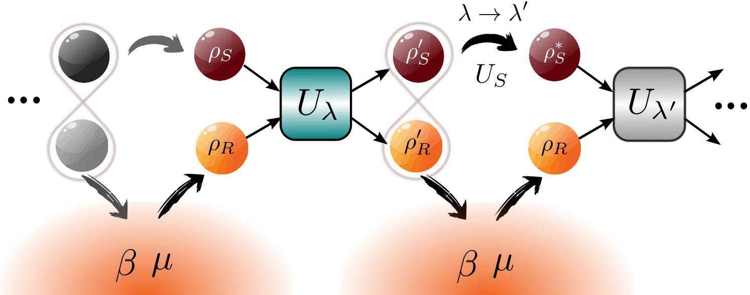
The key assumption of the dynamical evolution will be the presence of conserved quantities. The interaction between system and reservoir $H_{\mathrm{int}}$ should exactly preserve both energy and asymmetry in the global system at any time, that is $[H_{S}+H_{R},H_{\mathrm{int}}]=0$ and $[A_{S}+A_{R},H_{\mathrm{int}}]=0$. Here the asymmetry in the system $A_{S}$ is analogously defined as in Eq. (4) by $A_{S}(\lambda)\equiv-\hbar\omega_{\lambda}\left(a_{\lambda}^{\dagger 2}+a_{\lambda}^{2}\right)/2$ for any value of the external parameter $\lambda$. The later condition for the commutators leads to the conservation of total average energy and asymmetry for the first (interaction) step of the evolution:

where $\Delta E_{S}={\rm Tr}[H_{S}(\rho_{S}^{\prime}-\rho_{S})]$, $\Delta A_{S}={\rm Tr}[A_{S}(\rho_{S}^{\prime}-\rho_{S})]$ and analogously for the reservoir. It is worth noticing that this assumption indeed prevents extra sources of energy or asymmetry from switching on/off interactions considered in [44, 47].

Moreover, during the second step of the dynamical evolution energy and asymmetry may change due to the action of the external driving. Then on a coarse-grained time scale involving both first (interaction) and second (driving) steps, we have

where $\dot{W}={\rm Tr}[\dot{H}_{S}{\rho}_{S}]$ represents the mechanical work performed by the external driver, and analogously $\dot{\mathcal{A}}={\rm Tr}[\dot{A}_{S}{\rho}_{S}]$ is the asymmetry induced by driving. Now combining Eqs. (7) and (9) we state the first law of thermodynamics as

where $\dot{Q}\equiv-\dot{Q}_{R}$ is the heat entering the system and $\dot{W}_{\mathrm{sq}}\equiv-\dot{W}_{R}=-\mu\dot{A}_{R}$ is the chemical-like squeezing work performed by the reservoir.

Conservation of energy and asymmetry in Eqs. (8) is verified e.g. by prototypical beam splitter interactions of the form $H_{\mathrm{int}}\propto a_{\lambda}b_{k}^{\dagger}+a_{\lambda}^{\dagger}b_{k}$, as the ones typically assumed in derivations of the master equation for the squeezed thermal reservoir [6, 48, 49]. For frozen $\lambda$, contact with the reservoir brings any initial state of the system in the long time run to the equilibrium state

Here $\mathcal{S}_{\lambda}(\xi)=\exp[\frac{1}{2}\xi(a_{\lambda}^{2}-a_{\lambda}^{\dagger 2})]$ is the squeezing operator over the system mode, and $Z_{\lambda}={\rm Tr}[e^{-\beta(H_{S}-\mu A_{S})}]$. More generally, including the possibility of external driving into the system [Eq. (10)], the entropy production rate of a generic process as described previously can be calculated from the sum of von Neumann entropies of system and reservoir [27]. That results in the following statement of the second law

where $\dot{S}$ ($\dot{S}_{R}$) stands for the time-derivative of the von Neumann entropy of the system (reservoir). For the derivation of Eq. (12), we used the continuous version of Eq. (6) for the reservoir entropy changes, together with Eqs. (9) and (10).

Our objective now is to construct a generic reversible evolution for systems in contact with the squeezed thermal reservoir. We first consider the case of reversible work and asymmetry extraction by transforming an arbitrary initial state $\rho_{S}$ into the equilibrium state $\rho_{S}^{\mathrm{eq}}$ in Eq. (11). The transformation $\rho_{S}\rightarrow\rho_{S}^{\mathrm{eq}}$ might be done by simply letting the system relax in contact with the reservoir. However, this process is completely irreversible and prevent us from extracting any mechanical work nor asymmetry from $\rho_{S}$. On the contrary, a reversible protocol maximizing the extraction of resources can be built by extending the protocol explained in Ref. [36] for standard thermal reservoirs (see also Ref. [50]) to the case of a squeezed thermal reservoir.

This reversible process consists in two steps:

1. a)

   An initial sudden quench of the system Hamiltonian from $H_{S}(\lambda_{0})$ to $H_{S}({\lambda_{\ast}})\equiv H_{\ast}$, where

   $$~~~~H_{\ast}=\hbar\omega_{\lambda_{\ast}}a^{\dagger}_{\lambda_{\ast}}a^{~}_{\lambda_{\ast}}\equiv-\mathcal{S}^{\dagger}(\xi)\ln(\rho_{S})\mathcal{S}(\xi)/\beta_{0}.$$

   (13)

   This step is implemented by an instantaneous change in the control parameter $\lambda_{0}\rightarrow\lambda_{\ast}$, which implies as well $A_{S}(\lambda_{0})\rightarrow A_{S}(\lambda_{\ast})\equiv A_{\ast}$. The duration of this step is infinitesimal and, since the change in the control parameter is instantaneous, the system state does not change. Nevertheless, this initial quench is crucial for implementing a reversible transformation, as long as it leaves the system in equilibrium with the squeezed thermal reservoir, $\rho_{S}=\exp[{-\beta(H_{\ast}-\mu A_{\ast})}]/Z_{\ast}$, i.e. the state $\rho_{S}$ is now the equilibrium state of the system for $H_{\ast}$ and $A_{\ast}$. Notice that for performing this quench a work $W_{\mathrm{quench}}\equiv{\rm Tr}[(H_{\ast}-H_{S})\rho_{S}]$ and asymmetry $\mathcal{A}_{\mathrm{quench}}\equiv{\rm Tr}[(A_{\ast}-A_{S})\rho_{S}]$ are required, but no entropy is produced.

2. b)

   A reversible isothermal-like transformation where a quasi-static driving changes the Hamiltonian $H(\lambda_{\ast})$ and the asymmetry operator $A(\lambda_{\ast})$ back to their initial forms, while the system interacts with the reservoir. It is worth noticing that, since the system starts this step in equilibrium with the squeezed thermal reservoir, and the control parameter changes quasi-statically (infinitely slowly) from $\lambda_{\ast}$ to $\lambda_{0}$, the system will be maintained in equilibrium with the reservoir at any time [Eq. (11)], leaving the system in $\rho_{S}^{\mathrm{eq}}$. This implies zero entropy production during the process (reversibility), that is, $\dot{Q}=k_{B}T\dot{S}$ . In Appendix B we indicate a particular realization of this quasi-static process using a concatenation of CPTP maps.

In order to obtain a quantitative link between the work and asymmetry extractable from the initial state $\rho_{S}$, we may integrate Eq. (12) for reversible conditions (equality case) along the two steps of the protocol. For this purposes Eq. (12) can then be conveniently rewritten as

Integrating Eq. (14) and identifying $W_{\mathrm{ext}}=-W_{\mathrm{quench}}-\int_{\lambda_{\ast}}^{\lambda_{0}}{\rm Tr}[\dot{H}_{\lambda}\rho_{\lambda}^{\mathrm{eq}}]\mathrm{d}\lambda$ and $\mathcal{A}_{\mathrm{ext}}=-\mathcal{A}_{\mathrm{quench}}-\int_{\lambda_{\ast}}^{\lambda_{0}}{\rm Tr}[\dot{A}_{\lambda}\rho_{\lambda}^{\mathrm{eq}}]\mathrm{d}\lambda$ as the total work and asymmetry extracted in the process, we obtain

Here the quantity $\Omega(\rho_{S})\equiv{\rm Tr}[(H_{S}-\mu A_{S})\rho_{S}]-k_{B}TS(\rho_{S})$ is a potential generalizing the nonequilibrium free energy for systems interacting with a squeezed thermal reservoir. For obtaining (15) we used that ${\rm Tr}[(H_{S}-\mu A_{S})\rho_{S}^{\mathrm{eq}}]-k_{B}TS(\rho_{S}^{\mathrm{eq}})=-k_{B}T\ln Z_{\lambda}$. Moreover, in the last line we introduced the relative entropy $D(\rho||\sigma)={\rm Tr}[\rho(\ln\rho-\ln\sigma)]\geq 0$, which reaches zero if and only if $\rho=\sigma$ [51].

The interpretation of Eq. (15) may be now clarified by introducing the squeezing work performed by the reservoir, $W_{\mathrm{sq}}=\mu(\Delta A_{S}+\mathcal{A}_{\mathrm{ext}})$. We have:

Eq. (16) tell us that any out-of-equilibrium state $\rho_{S}\neq\rho_{S}^{\mathrm{eq}}$ is a resource which may be wasted in either extracting a positive net amount of work, $W_{\mathrm{ext}}-W_{\mathrm{sq}}$, or in increasing the asymmetry of the system, $\mu\Delta A_{S}$. Nevertheless, notice that even when our initial state is in equilibrium, $\rho_{S}=\rho_{S}^{\mathrm{eq}}$, extraction of mechanical work is not forbidden anymore, but it is allowed by cyclic extraction of asymmetry from the reservoir, $W_{\mathrm{ext}}=W_{\mathrm{sq}}=\mu\mathcal{A}_{\mathrm{ext}}$.

The previous protocol may be applied to more general transformations $\rho_{S}\rightarrow\rho_{S}^{\prime}$ by including slight modifications. In such case step a) is applied exactly as before, but in the quasi-static step b) we replace the final value of the control parameter by some $\lambda_{\ast}^{\prime}$ such that $H_{\ast}^{\prime}=H(\lambda_{\ast}^{\prime})\equiv-\mathcal{S}^{\dagger}(\xi)\ln(\rho_{S}^{\prime})\mathcal{S}(\xi)/\beta_{0}$. This implies that the system after quasi-static driving is now $\rho_{S}^{\prime}$. Then a final step is included: c) A final sudden quench $\lambda_{\ast}^{\prime}\rightarrow\lambda$ which instantaneously turns back the Hamiltonian and asymmetry operator to their original forms, $H_{S}$ and $A_{S}$. This extension is indeed equivalent to the combination of two reversible strokes, $\rho_{S}\rightarrow\rho_{\mathrm{eq}}$ as before, followed by the inversion of $\rho_{S}^{\prime}\rightarrow\rho_{\mathrm{eq}}$.

Once reversible protocols have been introduced we may now discuss work extraction from a single squeezed thermal reservoir. The idea is to introduce a thermodynamic cycle on the system which combines unitary processes on the system and interaction with the squeezed thermal reservoir. In Ref. [6], we already introduced a thermodynamic cycle for work extraction: 1) Starting with the system in $\rho_{S}^{\mathrm{eq}}$ in Eq. (11), the system is first detached from the reservoir and a unitary operation is implemented unsqueezing the mode $U_{1}=\mathcal{S}^{\dagger}$. This leaves the system in the state $\rho_{S}=e^{-\beta_{0}H_{S}}/Z$. 2) Then the squeezed thermal reservoir is reconnected and a simple relaxation take places, bringing the state of the system back to $\rho_{S}^{\mathrm{eq}}$. In such protocol, work is extracted in the first unitary stroke $W_{1}$, while the second stroke occurs in the absence of driving, and then the system only exchanges energy with the reservoir. Notice that this second relaxation step is intrinsically irreversible (isochoric process) and therefore it does not allow for an optimal use of the resources. Our aim here is to replace the isochoric process by a reversible process as introduced before.

Let us now generalize the previous two-stroke thermodynamic cycle for work extraction. 1) As before, the first stroke consist in detaching the system from the reservoir and implementing an arbitrary initial unitary step $U_{1}$, leaving the system in a rather arbitrary state $\rho_{S}$. During this stroke an amount of work $W_{1}={\rm Tr}[H_{S}(\rho_{S}^{\mathrm{eq}}-\rho_{S})]$ and asymmetry $\mathcal{A}_{1}={\rm Tr}[A_{S}(\rho_{S}^{\mathrm{eq}}-\rho_{S})]$ are extracted, while the entropy production is zero. 2) Now, for the second stroke we turn back to $\rho_{S}^{\mathrm{eq}}$ in contact with the environment, but also allowing arbitrary external driving. This eventually leads to extracting some extra amount of work $W_{2}$ during this step, together with asymmetry $\mathcal{A}_{2}$. For this second stroke we may apply Eq. (12). Integrating it and using that by construction $S(\rho_{S})=S(\rho_{S}^{\mathrm{eq}})$, $\Delta E_{S}=W_{1}$, and $\Delta A_{S}=\mathcal{A}_{1}$, a bound for the total work extracted $W_{\mathrm{ext}}=W_{1}+W_{2}$ is obtained

That is, in any cyclic process one may extract an amount of work less or equal than the squeezing chemical-like work performed by the reservoir. This indeed provides an extra motivation to consider $W_{\mathrm{sq}}$ as work and the squeezed thermal reservoir as a work producing reservoir [28].

The key point for reaching the equality in Eq. (17) is nothing but fully avoiding any irreversibility in the second stroke of the cycle. This is accomplished when this second stroke is exactly the (two-step) reversible process introduced below. Applying Eq. (15) it follows that $W_{2}=\Omega(\rho_{S})-\Omega(\rho_{S}^{\mathrm{eq}})+\mu\mathcal{A}_{2}=-W_{1}+\mu(\mathcal{A}_{1}+\mathcal{A}_{2})$, and the optimal amount of work $W_{\mathrm{ext}}=W_{1}+W_{2}=\mu(\mathcal{A}_{1}+\mathcal{A}_{2})=W_{\mathrm{sq}}$ is extracted. Furthermore, notice that this extraction protocol does not need any particular form of $\rho_{S}$ and $U_{1}$, e.g. we may use $U_{1}=\mathbb{I}$ [cf. Eq. (16)]. In any case, the chemical-like squeezing work extracted from the reservoir equals the asymmetry extracted by the external driver. Therefore, this can be regarded as an example of a squeezing into work conversion in the context of a generalized resource framework [22, 24].

Finally, it is worth mentioning that the maximum extractable work from a single reservoir $W_{\mathrm{sq}}$ is larger in general than the so-called ergotropy $\mathcal{W}$ of the non-passive state $\rho_{S}^{\mathrm{eq}}$ induced by the squeezed thermal reservoir. The later is defined as the maximum work extractable from a state using only unitary operations describing a cyclic variation of the Hamiltonian [52]. It can be straightforwardly seen that the ergotropy of the state $\rho_{S}^{\mathrm{eq}}$ is given by $W_{1}$ when $U_{1}=\mathcal{S}^{\dagger}$ [6]. We notice that this is just one part of the total extractable work, $W_{\mathrm{sq}}=W_{1}+W_{2}$, which can be made arbitrarily larger when increasing $\xi$ (see Fig. 2). In the following we provide explicit expressions for $\mathcal{W}$ and $W_{\mathrm{sq}}$.

Since $U_{1}=\mathcal{S}^{\dagger}$, leading to $\rho_{S}=U_{1}\rho_{S}^{\mathrm{eq}}U_{1}^{\dagger}=e^{-\beta_{0}H_{S}}/Z_{0}$, the work extracted in the first stroke explicitly reads:

where $n_{\mathrm{th}}=(e^{\beta_{0}\hbar\omega}-1)^{-1}$ is the mean number of excitations with energy $\hbar\omega$ in a thermal reservoir at $\beta_{0}$. Notice that $\rho_{S}$ is the Gibbs state, and then it is the state of lower energy for fix entropy. This implies that the work $W_{1}=\mathcal{W}$ is by definition the ergotropy of state $\rho_{S}^{eq}$. Moreover, during this stroke the asymmetry extracted reads

where $A_{0}\equiv A_{S}(\lambda_{0})$.

Next we calculate the work and asymmetry extracted in the second (two-steps) reversible stroke of the cycle. Following Eq. (13), in the first part of the stroke (sudden quench) the Hamiltonian is modified from $H_{0}$ to

where $b=S^{\dagger}(\xi)aS(\xi)$, while the state of the system does not change. At this point we can see that effectively after the quench we have $\rho_{S}=\mathcal{S}(\xi)e^{-\beta_{0}H_{\ast}}\mathcal{S}^{\dagger}(\xi)/Z_{0}$, which is the equilibrium state for Hamiltonian $H_{\ast}$. In this step the work extracted is

where we used Eq. (20). This means that the ergotropy extracted in the first stroke is wasted in implementing the initial sudden quench of the second stroke. Analogously, for the extracted asymmetry we have $\mathcal{A}_{2}^{\mathrm{quench}}=-\mathcal{A}_{1}$, so that until now we did not gained anything at all. Nevertheless, as we will shortly see, a greater amount of work and asymmetry is going to be extracted in the quasi-static step of the stroke. This can be implemented by means of the slow change of a control parameter $\lambda$ from $\lambda_{\ast}$ to $\lambda_{0}$, driving the Hamiltonian back to $H_{0}$. We will parametrize this process as an unsqueezing of the Hamiltonian

with $\lambda_{\ast}=\xi$ and $\lambda_{0}=0$. These operations are usually implemented in quantum optical setups like degenerate parametric down conversion by passing the light from a pumping laser field through a photonic crystal with $\chi^{(2)}$ nonlinearities (see e.g. [25, 53]). This kind of driving in particular implies that

where we used $\dot{b}_{\lambda}=-\dot{\lambda}b_{\lambda}^{\dagger}$, following Eq. (20). In the other hand, as shown in the previous section, the quasi-static driving implies the state of the system being at any time $\rho_{S}^{\mathrm{eq}}=\mathcal{S}(\xi)e^{-\beta_{0}H_{S}(\lambda)}\mathcal{S}^{\dagger}(\xi)/Z_{0}$. Therefore the work extracted during the quasi-static stroke reads

Analogously, for the extracted asymmetry we obtain

In conclusion, during a single cycle we obtain a total amount of extracted mechanical work and asymmetry

fulfilling $W_{\mathrm{ext}}=\mu\mathcal{A}_{\mathrm{ext}}$. Notice that the squeezing work in the setup is strictly greater than the ergotropy for any value of $\xi$, that is $W_{\mathrm{sq}}\equiv\mu\mathcal{A}_{\mathrm{ext}}>\mathcal{W}$, since $\xi\sinh(2\xi)>\sinh^{2}(\xi)~~\forall\xi>0$. This can be seen in Fig. 2 where $\mathcal{W}$ and $W_{\mathrm{sq}}$ are plotted as a function of $\xi$, in units of $\hbar\omega\coth(\beta_{0}\hbar\omega/2)$.

Finally, we point that one way of looking at the quantumness of the squeezing effects is to look at the induced uncertainty in position or momenta quadratures of our bosonic mode. In our case, for a squeezed thermal state, the squared uncertainty in the position quadrature $x=(1/\sqrt{2})(a+a^{\dagger})$ reads

and the Heisenberg uncertainty principle reads $\Delta x\Delta p\leq 1/2$. A genuine quantum state is then reached when this uncertainty falls below shot noise, i.e. when $\Delta x^{2}<1/2$. This is equivalent to squeezing the quadrature over a certain quantity

The quantity $\xi^{\ast}$ essentially depends on the relation between the magnitude of thermal fluctuations and the energy of the system. It diverges $\xi^{\ast}\rightarrow\infty$ for high temperatures $\beta_{0}\rightarrow 0$, while it approaches zero $\xi^{\ast}\rightarrow 0$, when the temperature goes to zero, $\beta_{0}\rightarrow\infty$. For a relevant parameter range $\beta_{0}\hbar\omega\simeq[0.01,1]$ we obtain values of $\xi^{\ast}$ from $2.65$ to $0.39$. As shown in Fig. 2, larger amounts of work can be obtained in the quantum regime $\xi>\xi^{\ast}$, where the uncertainty in the squeezed quadrature falls below shot noise.

In this paper we explored the interpretation of the squeezed thermal reservoir as a generalized equilibrium reservoir with two non-commuting charges: energy and (second-order moments) asymmetry. This identification can be done provided that the interaction with the reservoir preserve the two quantities, a condition easy to be fulfilled for the case of bosonic systems and in particular in the context of quantum optics (e.g. by a simple beam splitter interaction). Our formulation of the first and second laws of thermodynamics solve the major problem of how to correctly define work and heat for the squeezed thermal reservoir, but the same approach also applies to other non-thermal reservoirs such as the displaced thermal reservoir. In particular, our results show how previous approaches based on the naive consideration of any energy exchanged with the reservoir as heat [11, 12, 5, 6], or in the concept of ergotropy [7, 8] fail to provide a complete explanation of the energetics and thermodynamics. We expect that the identification of the chemical-like squeezing work provided here together with the generic reversible protocols may have a strong impact in new designs of quantum thermal machines or other devices combining thermal and squeezing effects.

References

- [1] J. Goold, M. Huber, A. Riera, L. del Rio, P. Skrzypczyk, The role of quantum information in thermodynamics: a topical review, J. Phys. A: Math. Theor. 49, 143001 (2016).
- [2] S. Vinjanampathy, and J. Anders, Quantum Thermodynamics, Contemp. Phys. 57, 545-579 (2016).
- [3] M. Lostaglio, D. Jennings, T. Rudolph, Quantum coherence, time-translation symmetry, and thermodynamics, Phys. Rev. X 5, 021001 (2015); M. N. Bera, A. Riera, M. Lewenstein, A. Winter, Generalized laws of thermodynamics in the presence of correlations, Nature Commun. 8, 2180 (2017).
- [4] L. del Rio, J. Aberg, R. Renner, O. Dahlsten, and V. Vedral, The thermodynamic meaning of negative entropy, Nature 474, 61-63 (2011); M. Perarnau-Llobet, K. V. Hovhannisyan, M. Huber, P. Skrzypczyk, N. Brunner, and A. Acín, Extractable work from correlations, Phys. Rev. X 5, 041011 (2015).
- [5] O. Abah and E. Lutz, Efficiency of heat engines coupled to nonequilibrium reservoirs, EPL 106, 20001 (2014).
- [6] G. Manzano, F. Galve, R. Zambrini, and J. M. R. Parrondo, Entropy production and thermodynamic power of the squeezed thermal reservoir, Phys. Rev. E 93, 052120 (2016).
- [7] W. Niedenzu, D. Gelbwaser-Klimovsky, A. G. Kofman, and G. Kurizki, On the operation of machines powered by quantum non-thermal baths, New. J. Phys. 18, 083012 (2016).
- [8] W. Niedenzu, V. Mukherjee, A. Ghosh, A. G. Kofman, and G. Kurizki, Quantum engine efficiency bound beyond the second law of thermodynamics, Nat. Commun. 9, 165 (2018).
- [9] M.O. Scully, M.S. Zubairy, G.S. Agarwal, and H. Walther, Extracting work from a single heat bath via vanishing quantum coherence, Science 299, 862-864 (2003).
- [10] R. Dillenschneider and E. Lutz, Energetics of quantum correlations, EPL 88, 5003 (2009).
- [11] X. L. Huang, T. Wang, and X. X. Yi, Effects of reservoir squeezing on quantum systems and work extraction, Phys. Rev. E 86, 051105 (2012).
- [12] J. Roßnagel, O. Abah, F. Schmidt-Kaler, K. Singer, and E. Lutz, Nanoscale heat engine beyond the Carnot limit, Phys. Rev. Lett. 112, 030602 (2014).
- [13] L. A. Correa, J. P. Palao, D. Alonso, and G. Adesso Quantum-enhanced absorption refrigerators, Sci. Rep. 4, 3949 (2014).
- [14] B. K. Agarwalla, J.-H. Jiang, and D. Segal, Quantum efficiency bound for continuous heat engines coupled to noncanonical reservoirs, Phys. Rev. B 96, 104304 (2017).
- [15] J. Klaers, S. Faelt, A. Imamoglu, and E. Togan, Squeezed thermal reservoirs as a resource for a nanomechanical engine beyond the Carnot limit, Phys. Rev. X 7, 031044 (2017).
- [16] J.M.R. Parrondo, B.J. de Cisneros, Energetics of Brownian motors: a review , App. Phys. A 75, 179-191 (2002).
- [17] U. Seifert, Efficiency of autonomous soft nanomachines at maximum power, Phys. Rev. Lett. 106, 020601 (2011).
- [18] D. Mandal and C. Jarzynski, Work and information processing in a solvable model of Maxwell’s demon, Proc. Natl. Acad. Sci. USA 109, 11641 (2012).
- [19] S. Deffner, and C. Jarzynski, Information processing and the second law of thermodynamics: An inclusive, Hamiltonian approach, Phys. Rev. X 3, 041003 (2013).
- [20] A. C. Barato and U. Seifert, Stochastic thermodynamics with information reservoirs, Phys. Rev. E 90, 042150 (2014).
- [21] E. T. Jaynes, Information theory and statistical mechanics, Phys. Rev. 106, 620 (1957); Information theory and statistical mechanics II, Phys. Rev. 108, 171 (1957).
- [22] Y. Gurnayova, S. Popescu, A. Short, R. Silva, and P. Skrzypczyk, Thermodynamics of quantum systems with multiple conserved quantities, Nat. Commun. 7, 12049 (2016).
- [23] N. Y. Halpern, P. Faist, J. Oppenheim, and A. Winter, Microcanonical and resource-theoretic derivations of the thermal state of a quantum system with noncommuting charges, Nat. Commun. 7, 12051 (2016).
- [24] M. Lostaglio, D. Jennings, and T. Rudolph, Thermodynamic resource theories, non-commutativity and maximum entropy principles, New J. Phys. 19 043008 (2017).
- [25] P. D. Drummond and Z. Ficek (Eds.), Quantum squeezing (Springer-Verlag, Berlin Heidelberg, 2004).
- [26] E. S. Polzik, The squeeze goes on, Nature 453, 45-46 (2008).
- [27] G. Manzano, J. M. Horowitz, and J. M. R. Parrondo, Quantum fluctuation theorems for arbitrary environments: adiabatic and non-adiabatic entropy production, Phys. Rev. X 8, 031037 (2018).
- [28] J. M. Horowitz and M. Esposito, Work producing reservoirs: Stochastic thermodynamics with generalized Gibbs ensembles, Phys. Rev. E 94, 020102(R) (2016).
- [29] H. Fearn and M. J. Collett, Representations of squeezed states with thermal noise, J. Mod. Opt. 35, 553 (1988).
- [30] M. Rigol, V. Dunjko, V. Yurovsky, and M. Olshanii, Relaxation in a completely integrable many-body quantum system: An ab initio study of the dynamics of the highly excited states of 1D lattice hard-core bosons Phys. Rev. Lett. 98, 050405 (2007).
- [31] J.A. Vaccaro and S. M. Barnett, Information erasure without an energy cost, Proc. R. Soc. A 467, 1770-1778 (2011); S. M. Barnett and J.A. Vaccaro, Beyond Landauer erasure, Entropy 15, 4956-4968 (2013).
- [32] T. Langen, S. Erne, R. Geiger, B. Rauer, T. Schweigler, M. Kuhnert, W. Rohringer, I. E. Mazets, T. Gasenzer, and J. Schmiedmayer, Experimental observation of a generalized Gibbs ensemble, Science 348, 207-211 (2015).
- [33] M. Perarnau-Llobet, A. Riera, R. Gallego, H. Wilming and J. Eisert, Work and entropy production in generalised Gibbs ensembles, New J. Phys. 18, 123035 (2016).
- [34] Y.-K. Liu, Gibbs states and the consistency of local density matrices, arXiv:quant-ph/0603012 (2006).
- [35] M. S. Kim, F. A. M. de Oliveira, and P. L. Knight, Properties of squeezed number states and squeezed thermal states, Phys. Rev. A 40, 2494 (1989).
- [36] J. M. R. Parrondo, J. M. Horowitz and T. Sagawa, Thermodynamics of information, Nat. Phys. 11, 131-139 (2015).
- [37] P. Skrzypczyk, A. J. Short, and S. Popescu, Work extraction and thermodynamics for individual quantum systems, Nature Commun. 5, 4185 (2014).
- [38] R. Gallego, J. Eisert and H. Wilming, Thermodynamic work from operational principles, New J. Phys. 18 103017 (2016).
- [39] Notice that since this “fresh” mode is freely provided by the reservoir, the replacement does not incurs in any extra energetic cost. Moreover, since the state of the whole reservoir changes only infinitesimally due to the interaction with the system, no extra entropy is produced [27].
- [40] V. Scarani, M. Ziman, P. Stelmachovic, N. Gisin, and V. Buzek, Thermalizing quantum machines: dissipation and entanglement, Phys. Rev. Lett. 88, 097905 (2002).
- [41] S. Lorenzo, R. McCloskey, F. Ciccarello, M. Paternostro, and G. M. Palma, Landauer’s Principle in Multipartite Open Quantum System Dynamics, Phys. Rev. Lett. 115, 120403 (2015).
- [42] G. Manzano, J. M. Horowitz, and J. M. R. Parrondo, Nonequilibirum potential and flucutation theorems for quantum maps, Phys. Rev. E 92, 032129 (2015).
- [43] F.Barra, and C. Lledó, Stochastic thermodynamics of quantum maps with and without equilibrium, Phys. Rev. E 96, 052114 (2017).
- [44] P. Strasberg, G. Schaller, T. Brandes, M. Esposito, Quantum and information thermodynamics: a unifying framework based on repeated interactions, Phys. Rev. X 7, 021003 (2017).
- [45] J. M. Horowitz, Quantum-trajectory approach to the stochastic thermodynamics of a forced harmonic oscillator, Phys. Rev. E 85, 031110 (2012).
- [46] J. M. Horowitz and J. M. R. Parrondo, Entropy production along nonequilibrium quantum jump trajectories, New J. Phys. 15, 085028 (2013).
- [47] F. Barra, The thermodynamic cost of driving quantum systems by their boundaries, Sci. Rep. 5, 14873 (2015).
- [48] D. F. Walls and G. J. Milburn, Quantum Optics (Springer, Berlin, 1994).
- [49] M. O. Scully and M. S. Zubairy, Quantum Optics (Cambridge University Press, Cambridge, 1997).
- [50] G. Manzano, F. Plastina, and R. Zambrini, Optimal work extraction and thermodynamics of quantum measurements and correlations, Phys. Rev. Lett. 121, 120602 (2018).
- [51] T. Sagawa, Second law-like inequalitites with quantum relative entropy: An introduction, in Lectures on quantum computing, thermodynamics and statistical physics, Kinki University Series on Quantum Computing, Vol. 8 (World Scientic, New Jersey, 2013).
- [52] A. E. Allahverdyan, R. Balian, and Th. M. Nieuwenhuizen, Maximal work extraction from finite quantum systems, EPL 67, 565 (2004).
- [53] C. C. Gerry and P. L. Knight, Introductory Quantum Optics (Cambridge University Press, 2005).
- [54] H. T. Quan, S. Yang, and C. P. Sun, Microscopic work distribution of small systems in quantum isothermal processes and the minimal work principle, Phys. Rev. E 78, 021116 (2008).