Private Text Classification: Using Radomacher operators and blind addition to allow multiple peers to learn text without seeing the text

Leif W. Hanlen Richard Nock Hanna J. Suominen Neil Bacon Correspondence to: leif.hanlen@gmail.com

Abstract

Confidential text corpora exist in many forms, but do not allow arbitrary sharing. We construct typical text processing applications using appropriate privacy preservation techniques (including homomorphic encryption, Rademacher operators and secure computation). We set out the preliminary materials from Rademacher operators for binary classifiers, and then construct basic text processing approaches to match those binary classifiers.

Keywords:

Machine Learning, Private, Text Analytics, NLP

⁰⁰footnotetext: Leif W. Hanlen is with CSIRO, Data61, and Australian National University and University of Canberra. Richard Nock and Neil Bacon are with CSIRO, Data61. Hanna J. Suominen is with CSIRO, Data61, University of Canberra, Australian National University, University of Turku, and University of Canberra.

1 Motivation

Private text data — with confidential content — is difficult to “open”. Privacy requirements in text data are difficult to guarantee due to the inter-dependencies of text, and grammar. Although Natural Language Processing (NLP) nominally operates on numerically encoded text, NLP exploits the structure of text and not merely a sequence of integer codes (Hirschberg & Manning, 2015).

Research work in the space of Information Retrieval (IR) has acknowledged the need to preserve privacy (Si et al., 2014; Oard, 2015). Mechanisms to accommodate sharing of text corpora, have essentially reduced to licensing requirements that allow full access under limited conditions of (re-)use, since sharing (raw) text data essentially allows a human to read (and reproduce) the data (Dankar & Emam, 2013; Thomson, 2004; Ji et al., 2014; McDonald & Kelly, 2012).

1.1 Machine Learning from Private Text Data

The (typical) components of the text document that might be subject to privacy concerns (names of persons, places, drug-names, disease-names) are likely to be the components most interesting for text processing — and most damaging to algorithm performance if altered. In this work, we consider a different approach: we apply encryption techniques to text which allow learning without viewing the raw data — thereby applying machine learning without the need to share (or read) text data to learn from private text corpora and classify private text.

This work does not avoid the need for ethical approval and research permission: encryption and privacy preserving techniques cannot overcome ethical, legislative, or contractual requirements on what may (or may not) be done with data. We are interested in allowing groups to ethically interact with data, where raw data sharing would not be desired (or possible).

1.1.1 Text in Health Is a Special Case

Although open sharing is generally accepted as a good principal in health (Verhulst et al., 2014; Dunn et al., 2012; Estrin & Sim, 2010; Veitch & Barbour, 2010); privacy concerns may overwhelm implied scientific benefit (Thomson, 2004; Vogel, 2011; Sayogo & Pardo, 2012). The need to address privacy while supporting research-use (as well as non-research use) of health data has been observed (McKeon et al., 2013). To support confidentiality, the British Medical Journal [Table 1 (Hrynaszkiewicz et al., 2010) recommends not publishing verbatim responses or transcriptions of clinical discussions — which is exactly the sort of data that text mining systems require (Suominen et al., 2014; Suominen et al., 2015). The work of (Jin, 2007) suggests some approaches for privacy-preserving health analytics, and reviews several privacy-preserving techniques, although most are numeric focused.

The risk of compromising privacy by being able to conceal the identifiers remains regardless of recent advances in automated de-identification algorithms for health text. Algorithms for automated de-identification of health text have have been evaluated to reach the F1 correctness percentage from 81 to 99 in English, French, Japanese, and Swedish (Dalianis & Velupillai, 2010; Morita et al., 2013; Chazard et al., 2013; Grouin & Neveol, 2014; Kayaalp et al., 2014; Meystre et al., 2014).¹¹ 1 F1 is a performance measure that takes values between 0 and 1 — the larger the value, the better the performance. It is defined as the harmonic mean of precision and recall, that is, $2\times(\textrm{precision}\times\textrm{recall})/(\textrm{precision}+\textrm{recall})$ where precision refers to the proportion of correctly identified words for de-identification to all de-identified words and recall refers to the proportion of correctly identified words for de-identification to all words that should have been de-identified. However, approximately 90 per cent of the residual identifiers left behind by either these algorithms or human coders can be concealed by applying additional computation methods (Carrell et al., 2013).

This capability to conceal the identifiers gets even more alarming after record linkage of different shared corpora. For example, in the USA, Washington is one of 33 states that share or sell anonymized patient records. For US$50, anyone can purchase a patient-level health corpus that contains all hospitalisations that occurred in this state in 2011, without patient names or addresses, but with full patient demographics, diagnoses, procedures, attending physician, hospital, a summary of charges, and how the bill was paid. By linking these de-identified health records with public news papers from the same year from Washington State, leads 43 per cent of the time to concealing the patient’s name and sometimes even her/his street address (Sweeney, 2015),

As expected, patients are concerned about the potential of health data sharing and linkage to result in data misuse and compromised privacy (Simon et al., 2009). However, they are also enthusiastic about their capacity to improve the quality and safety of health care through giving their informed consent to sharing some or all of their own health records for purposes of (medical) science in general or some specific research project (Shaw et al., 2016).

Our approach addresses precisely these problems in finding and “hiding” sensitive text. It allow machine learning algorithms to use all encrypted data, but not all raw text.

2 Background

We assume all participants are Honest But Curious (HBC) (Paverd et al., 2014). We limit the need for “trusted” intermediaries (Dwork & Roth, 2014), and where such intermediaries are used, we restrict (by aggregation and secure computing) the information they may receive.

2.1 Text Processing

We consider the typical linear so-called “1-best” pipeline as outlined in (Johnson, 2014). This could be extended to parallel, iterative, or network approaches. We shall ignore feature engineering and simply presume a (large) number of categorical variables. A particular example of text processing pipeline output is outlined in Figure 1 of (Hirschberg & Manning, 2015).

In training, the text processing pipeline also uses labelled text segments — which may be document-, sentence- or word- labels (e.g. for sentiment analysis) or some combination of text fragments (such as used by the Browser Rapid Annotation Tool (BRAT) for collaborative text annotation (Stenetorp et al., 2012)). In each case, we may represent the features as numeric labels — where the “tags” are converted into a dictionary — and a series of numeric values. We shall be interested in binary values — such as might result from a “1-hot” encoding. These become our observations, and also labels.

A differential-privacy approach is not suitable for this data type: adding “noise” to the encoded text will either render the “new” text meaningless, or be overcome — by treating the noise as spelling or grammatic errors. We use the approach of (Shannon, 1949) — to improve independent secret systems by concatenating them. In this case, we will firstly encrypt the numeric features and labels (using a Paillier homomorphic encryption system (Paillier, 1999; Damgård & Jurik, 2001)). This makes direct interpretation difficult. Second, we attempt to address the data dependencies by applying irreversible aggregation to the numeric data so as to hide many of the implied dependencies between observations. Finally, we wrap the learning process in a secure learning approach, to further reduce the capacity of an inquisitive user discovering the underlying labels. This reflects the well known fact that data dependences must be accounted for in training, validation, and testing of machine learning methods in order to produce reliable performance estimates (Suominen et al., 2008; Pahikkala et al., 2012).

Figure 1: Text processing pipeline with encryption, pre-processing is encapsulated in the dashed arrow.

2.2 Partial Homomorphic Encryption

The Paillier encyption scheme (Paillier, 1999) (and later generalisations (Damgård & Jurik, 2001)) is a public-private key encryption scheme. We alter the notation of (Franz, 2011) (note, this is different to (Djatmiko et al., 2014)) where an integer $x$ is encrypted as ${\left\langle\!\left\langle x\right\rangle\!\right\rangle}$ and the decrypt operation is ${\left\langle\!\left\langle y\right\rangle\!\right\rangle^{-1}}$ . In other words,

x\stackrel{{\scriptstyle\text{encrypt}}}{{\longmapsto}}{\left\langle\!\left\langle x\right\rangle\!\right\rangle}\stackrel{{\scriptstyle\text{decrypt}}}{{\longmapsto}}{\left\langle\!\left\langle{\left\langle\!\left\langle x\right\rangle\!\right\rangle}\right\rangle\!\right\rangle^{-1}}=x.

(1)

The operations ${\left\langle\!\left\langle\cdot\right\rangle\!\right\rangle}$ and ${\left\langle\!\left\langle\cdot\right\rangle\!\right\rangle^{-1}}$ in Definition (1) are public key encryptions: users can encrypt data (and perform computations) using a common public key, however, only the user with the corresponding private key can extract the clear data.

The main operations for Paillier homomorphic encryption are the operators $\oplus$ and $\otimes$ . They are defined for two integers $x_{1},x_{2}<n=pq$ where $n$ is a constant for the particular encryption and parameters $p$ and $q$ are two large primes as follows:

{\left\langle\!\left\langle x_{1}\right\rangle\!\right\rangle}\oplus{\left\langle\!\left\langle x_{2}\right\rangle\!\right\rangle}={\left\langle\!\left\langle x_{1}+x_{2}\right\rangle\!\right\rangle}

(2)

and

\alpha\otimes{\left\langle\!\left\langle x_{2}\right\rangle\!\right\rangle}={\left\langle\!\left\langle\alpha\cdot x_{2}\right\rangle\!\right\rangle}

(3)

where $\alpha$ is an un-encrypted real-valued scalar.

Equations (2) and (3) gain us an ability to sum encrypted values in the encrypted domain (and consequently decrypt the result) and multiply encrypted values with un-encrypted scalars. Note that the result (3) does not apply when $\alpha$ is encrypted. For more advanced operations (such as multiplying encrypted values) we use secure computation.

2.3 Secure Computations

We use results from (Franz, 2011; From & Jakobsen, 2006) to provide several protocols for secure computation among two parties $\mathcal{A}$ and $\mathcal{B}$ . Work from (Clifton et al., 2002) provides mechanism for multiple parties (i.e., more than two). We shall assume that $\mathcal{A}$ operates on encrypted data, and $\mathcal{B}$ has the private key (and can decrypt data). Neither party should be able to discern the numerical values. These protocols comprise the following three steps:

1.

an obfuscation step by the public key holder $\mathcal{A}$ ,
2.

a transfer step to the private key holder $\mathcal{B}$ , who decrypts and then performs the calculation on clear data²² 2 As the result is obfuscated, $\mathcal{B}$ learns nothing from this operation, even though it is performed on clear data. and returns an encrypted result to $\mathcal{A}$ , and
3.

$\mathcal{A}$ then removes the original obfuscation.

Other work extends (Franz, 2011) to linear algebra for homomorphic analysis.

We now recall the work of (Nock et al., 2015) and (Patrini et al., 2016) to present relevant parts the aggregation techniques. This presents learners on specially aggregated data sets where the data set could be in a single location.

2.3.1 Single (Complete) Data Set

We will first consider the data set as a single (coherent) source. That is, all data is held by a single organisation.

Definition 1 ((Numeric) Supervised Learning Space).

Given a set of $m>0$ examples $\mathcal{S}=\left\{({\boldsymbol{x}}_{i},y_{i}),i\in\{1,2,\ldots,m\}\right\}$ , where ${\boldsymbol{x}}_{i}\in\mathcal{X}\subseteq\Real^{1\times d}$ are observations, $\mathcal{X}$ is the domain, and $y_{i}\in\{-1,1\}$ are binary labels. We are concerned with a (binary) linear classifier ${\boldsymbol{\theta}}\in\Theta$ for fixed $\Theta\subseteq\Real^{1\times d}$ . The label of an observation ${\boldsymbol{x}}$ is given by

\mathrm{label}({\boldsymbol{x}})=\sign\left({\boldsymbol{\theta}}^{T}{\boldsymbol{x}}\right)\in\{-1,1\}.

The irreversible aggregation is based on Rademacher observations (rados) as defined below:

Definition 2 (Rado).

cf.Definition 1 (Nock et al., 2015)

Let $\Sigma=\{-1,1\}^{n}$ . Then given a set of $\mathcal{S}$ , and for any ${\boldsymbol{\sigma}}\in\Sigma$ with ${\boldsymbol{\sigma}}=[\sigma_{1},\ldots,\sigma_{n}]^{T}$ . The Rademacher observation ${\boldsymbol{\pi}}_{\boldsymbol{\sigma}}$ with signature ${\boldsymbol{\sigma}}$ is

{\boldsymbol{\pi}}_{\boldsymbol{\sigma}}=\frac{1}{2}\sum_{i=1}^{n}(\sigma_{i}+y_{i}){\boldsymbol{x}}_{i}.

(4)

2.3.2 Multiple Data Sets

This case is described in Figure 1 (Patrini et al., 2016). We do not assume that entities are linked: different text corpora are held by different parties, and no entity resolution is performed.

Definition 3 (BB-Rado).

cf. Definition 1 (Patrini et al., 2016) Consider ${\boldsymbol{z^{\prime}}}\in U\subset V$ . Let $\mathrm{lift}({\boldsymbol{z^{\prime}}})$ concatenate zeros to ${\boldsymbol{z}}=[{\boldsymbol{z^{\prime}}}\ {\boldsymbol{0}}]$ such that ${\boldsymbol{z}}\in V$ . For any ${\boldsymbol{s}}\in\mathcal{J}$ , labels $y\in\{-1,1\}$ and $\alpha\in\Real$ , the $\alpha$ -basic block rado for $({\boldsymbol{s}},y)$ is

{\boldsymbol{\pi}}^{\alpha}_{({\boldsymbol{s}},y)}\stackrel{{\scriptstyle\cdot}}{{=}}\alpha\cdot\mathrm{lift}(y\cdot{\boldsymbol{s}})+\sum_{j=1}^{p}\mathrm{lift}\left({\boldsymbol{\pi}}^{j}_{({\boldsymbol{s}},y)}\right).

(5)

2.4 Encrypted Rados

The encryption process occurs after securely processing the text documents at the private location of $\mathcal{B}$ . Using her/his private key, $\mathcal{B}$ then encrypts the features, and these are then aggregated. The aggregation occurs blind to $\mathcal{B}$ , and may be performed by an honest-but-curious intermediary $\mathcal{I}_{\mathcal{B}}$ . The rados ${\boldsymbol{\pi}}_{\boldsymbol{\sigma}}$ are generated privately at $\mathcal{I}_{\mathcal{B}}$ . Once generated, the rados can be used by other honest-but-curious external parties $\mathcal{A}$ .

Figure 2 outlines the encryption steps, using secure mathematical operations, and denote the two parties as $\{\mathcal{B},\mathcal{I}\}$ where $\mathcal{B}$ is the private key holder and $\mathcal{I}$ is an intermediary. $\mathcal{I}$ can “see” encrypted features ${\left\langle\!\left\langle{\boldsymbol{{\boldsymbol{x}}}}_{i}\right\rangle\!\right\rangle}$ , and encrypted labels ${\left\langle\!\left\langle y_{i}\right\rangle\!\right\rangle}$ , and knows the choices of rado vectors (i.e., $\mathcal{I}$ knows values of $\sigma_{i}$ ). It would be possible to operate with $\sigma_{i}$ also encrypted.

We re-write Equation (4) below with the encrypted values made explicit. Corresponding secure mathematical operations are also shown. We use the notation $\bigoplus_{i=1}^{n}$ to denote a series of homomorphic addition operations ie. $\bigoplus_{i=1}^{n}=a_{1}\oplus a_{2}\oplus\cdots\oplus a_{n}$ . We will use $:$ as an abuse of notation, to denote “has the meaning of” rather than equality, as follows:

{\left\langle\!\left\langle{\boldsymbol{\pi}}_{\boldsymbol{\sigma}}\right\rangle\!\right\rangle}\quad:\quad\frac{1}{2}\sum_{i=1}^{m}\left(\sigma_{i}+{\left\langle\!\left\langle y_{i}\right\rangle\!\right\rangle}\right){\left\langle\!\left\langle{\boldsymbol{x}}_{i}\right\rangle\!\right\rangle}.

(6)

The resulting “Equation” (6) shows the formation of the (encrypted) rado. The additions and (unencrypted scalar) multiplications must all be translated to the appropriate homomorphic addition and multiplication operations.

The output is an encoded rado, based on any numerical field, that we will refer to as ${\left\langle\!\left\langle{\boldsymbol{\pi_{\sigma}}}\right\rangle\!\right\rangle}$ . We outline the procedure to build the rado in Protocol 1: 1Encrypted Radomacher.

Protocol 1 Encrypted Radomacher

{\left\langle\!\left\langle{\boldsymbol{\pi_{\sigma}}}\right\rangle\!\right\rangle}

at peer

{\boldsymbol{\sigma}}\stackrel{{\scriptstyle\text{encrypt}}}{{\longmapsto}}{\left\langle\!\left\langle{\boldsymbol{\sigma}}\right\rangle\!\right\rangle}

{\left\langle\!\left\langle{\boldsymbol{\phi}}\right\rangle\!\right\rangle}\leftarrow{\left\langle\!\left\langle{\boldsymbol{\sigma}}\right\rangle\!\right\rangle}\oplus{\left\langle\!\left\langle{\boldsymbol{y}}\right\rangle\!\right\rangle}

{\left\langle\!\left\langle{\boldsymbol{\phi}}\right\rangle\!\right\rangle}\leftarrow\frac{1}{2}\otimes{\left\langle\!\left\langle{\boldsymbol{\phi}}\right\rangle\!\right\rangle}

{\left\langle\!\left\langle{\boldsymbol{\pi_{\sigma}}}\right\rangle\!\right\rangle}\leftarrow

S.InnerProd(

{\left\langle\!\left\langle{\boldsymbol{\phi}}\right\rangle\!\right\rangle},{\left\langle\!\left\langle{\boldsymbol{x}}\right\rangle\!\right\rangle}

)

2.4.1 Multi-party Case

The case for multiple parties requires the use of the $\mathrm{lift}(\cdot)$ function. This function appends zeros onto a vector, and thus (in the encrypted domain) may be represented as appending an encrypted scalar (zero) to the encrypted vector. As above, Equation (5) can be re-written in the encrypted domain.

Figure 2: Feature encryption pipeline, showing encryption links and (dashed) knowledge at

\mathcal{B}

with private key, and intermediary

\mathcal{I}_{\mathcal{B}}

2.5 Learning, Using Encrypted Rados

2.5.1 Unencrypted Single-party Case

Recall the learner for rados (in the unencrypted case) is given by (Nock et al., 2015). We will use the equivalent (exponential) learner for rados as follows:

Lemma 1 (Rado Learning).

(cf. Lemma 2 (Nock et al., 2015) ) For any ${\boldsymbol{\theta}}$ and $\mathcal{S}$ , and a set of rados ${\boldsymbol{\sigma}}\in\mathcal{U}\subseteq\Sigma$ , minimizing the loss

\log\left[F_{\exp}(\mathcal{S},{\boldsymbol{\theta}})\right]=\log\left[\frac{1}{n}\sum_{{\boldsymbol{\sigma}}\in\mathcal{U}}\exp\left(-{\boldsymbol{\theta}}^{T}{\boldsymbol{\pi}}_{\boldsymbol{\sigma}}\right)\right]

(7)

is equivalent to minimising the standard logistic loss $F_{\log}(\mathcal{S},{\boldsymbol{\theta}})$ .

The supervised learning (optimisation) is written as

Problem 1 (Minimise Exponential Loss).

The optimal classifier ${\boldsymbol{\theta}}^{*}$ is given by solving

{\boldsymbol{\theta}}^{*}=\min_{\boldsymbol{\theta}}J({\boldsymbol{\theta}})

(8)

where

J({\boldsymbol{\theta}})=\log\left[\frac{1}{n}\sum_{{\boldsymbol{\sigma}}\in\mathcal{U}}\exp\left(-{\boldsymbol{\theta}}^{T}{\boldsymbol{\pi}}_{\boldsymbol{\sigma}}\right)\right]+{\boldsymbol{\theta}}^{T}{\boldsymbol{\theta}}

(9)

and ${\boldsymbol{\theta}}^{T}{\boldsymbol{\theta}}$ is a regularising term (a.k.a. regulariser).

2.5.2 Secure Single-party Case

The exponential in Equation (9) can be computed securely using the protocol outlined in (Yu et al., 2011). The logarithm can be performed using Algorithm 1 (Djatmiko et al., 2016). We perform a gradient descent to solve Problem 1.

Recall Problem 1. Note that the gradient of $J({\boldsymbol{\theta}})$ , with respect to $\theta_{j}$ , is

\frac{\partial}{\partial\theta_{j}}J({\boldsymbol{\theta}})=\frac{\sum_{\boldsymbol{\pi}}-\pi_{j}\exp\left(-\sum_{i}\theta_{i}\pi_{i}\right)}{\sum_{\boldsymbol{\pi}}\exp\left(-\sum_{i}\theta_{i}\pi_{i}\right)}+2\theta_{j}.

(10)

We note that ${\left\langle\!\left\langle{\boldsymbol{\pi}}\right\rangle\!\right\rangle}\in\mathcal{P}$ .

Using our abuse of notation $:$ we have

{\left\langle\!\left\langle J({{\boldsymbol{\theta}}})\right\rangle\!\right\rangle}\ :\ \left[\sum_{j}-\pi_{j}\exp\left(-\sum_{i}\theta_{i}\pi_{i}\right)\right].

(11)

2.5.3 Unencrypted, Multi-party Case

The proof of Theorem 3 (Patrini et al., 2016) shows that the mean square loss can be used, over $\mathcal{P}$ — that is, on the limited sample sets — by using a modified mean loss as given in Definition 4 as follows:

Definition 4 (BB-Rado loss).

cf. Definition 2 .(Patrini et al., 2016) and Theorem 3 (Patrini et al., 2016) The $M$ -loss for the classifier ${\boldsymbol{\theta}}$ is

\ell_{M}(\mathcal{R}_{S,\mathcal{P}})\stackrel{{\scriptstyle\cdot}}{{=}}-\left(\expect_{\mathcal{P}}\left[{\boldsymbol{\theta}}^{T}{\boldsymbol{\pi}}_{\boldsymbol{\sigma}}\right]-\frac{1}{2}\variance_{\mathcal{P}}\left[{\boldsymbol{\theta}}^{T}{\boldsymbol{\pi}}_{\boldsymbol{\sigma}}\right]\right)\\ +\frac{m}{4}{\boldsymbol{\theta}}^{T}\Gamma{\boldsymbol{\theta}}

(12)

where expectation $\expect_{\mathcal{P}}$ and variance $\variance_{\mathcal{P}}$ are computed with respect to the uniform sampling of $\sigma$ in $\mathcal{P}$ . If the matrix $\Gamma$ is positive definite, it can be defined as a weighted diagonal matrix

\Gamma=\begin{bmatrix}I_{m}&{\boldsymbol{0}}_{m}\\ {\boldsymbol{0}}_{n}&\epsilon I_{n}\end{bmatrix}

(13)

where $0<\epsilon\ll 1$ accounts for (lack of) confidence in certain columns of ${\boldsymbol{\pi}}$ .

“[M]inimizing the Ridge regularized square loss over examples is equivalent to minimizing a regularized version of the M-loss, over the complete set of all rados.” (Patrini et al., 2016)

The optimal classifier ${\boldsymbol{\theta}}^{\star}$ is given by the simple closed-form expression Theorem 6 (Patrini et al., 2016). Namely,

{\boldsymbol{\theta}}^{\star}=\left(BB^{T}+\mathrm{dim}_{c}(B)\cdot\Gamma\right)^{-1}B{\boldsymbol{1}}

(14)

where $B$ is stacked (column-wise) rados and $\mathrm{dim}_{c}(B)$ is the number of columns of $B$ . The procedure for building the rados and solving for ${\boldsymbol{\theta}}$ are given in (Patrini et al., 2016).

To solve (14), (Hall et al., 2011 (revised 2013) recommends an iterative – Shur (Guo & Higham, 2006)) approach. Faster approaches (with fewer multiplications) are achieved by higher order algorithms. An outline and review are given in (Rajagopalan, 1996; Soleymani, 2012). The inverse may be found using secure multiplication linear algebra.

2.5.4 De-risking the Coordinator

The notation of (Patrini et al., 2016) suggests a central coordinator with access to all vectors,: we avoid this by returning to Definition 4. Let

{\boldsymbol{b}}=\sum_{{\boldsymbol{\pi}}\in\mathcal{P}}{\boldsymbol{\pi}}=\expect_{\mathcal{P}}\left({\boldsymbol{\pi}}_{\boldsymbol{\sigma}}\right)

(15)

and then

\frac{\partial\ell}{\partial{\boldsymbol{\theta}}}=-{\boldsymbol{b}}^{T}+{\boldsymbol{\theta}}^{T}\left[\Gamma+\frac{1}{2}\sum_{{\boldsymbol{\pi}}\in\mathcal{P}}\left({\boldsymbol{\pi}}-{\boldsymbol{b}}\right)\left({\boldsymbol{\pi}}-{\boldsymbol{b}}\right)^{T}\right].

(16)

The sums in Equations (15) and (16) are over the appropriate rados. However, these rados may be calculated by their peers, so the sums may be broken into per-peer summations, where we consider disjoint sets $\mathcal{P}_{p}$ such that $\mathcal{P}_{1}\cup\mathcal{P}_{2}\cup\ldots=\mathcal{P}$ .

Definition 5 (BB-rado per peer).

Consider $P$ peers with $p\in\{1,2,\ldots,P\}$ , where each peer $p$ has distinct rados drawn from $\mathcal{P}_{p}$ , and the rados are distinct in $\mathcal{P}_{1}\cup\mathcal{P}_{2}\cup\ldots=\mathcal{P}$ . For each peer $p$ , we have a expectation ${\boldsymbol{e}}_{p}$ and variance ${\boldsymbol{v}}_{p}$ defined as

{\boldsymbol{e}}_{p}=\sum_{\mathcal{P}_{p}}{\boldsymbol{\pi}}_{i}

(17)

and

{\boldsymbol{v}}_{p}=\sum_{\mathcal{P}_{p}}\left({\boldsymbol{\pi}}_{i}-{\boldsymbol{b}}\right)\left({\boldsymbol{\pi}}_{i}-{\boldsymbol{b}}\right)^{T}.

(18)

Each peer $p$ can calculate ${\boldsymbol{e}}_{p}$ and ${\boldsymbol{v}}_{p}$ independently.

Although the mean ${\boldsymbol{b}}$ may be calculated centrally, it is preferable to use secure multi-party addition to achieve the same result. This reduces the scope for the coordinator to access (encrypted, aggregated) vectors, and (instead) only access noisy aggregates of the data.

3 Putting the Bricks together

The algorithm incorporates the secure multi-party summation work of (Clifton et al., 2002), to prevent the coordinator from obtaining the rados directly. This adds a third layer of obfuscation to the data (encryption, aggregation, blind addition), which means that at the coordinator (who can decrypt the data) the data remains protected by the aggregation to rados and the blind addition of the vectors.

Protocol 2 Classifier for Secure Text with Central Coordinator

0: peers

p\in\{1,\ldots,P\}

, coordinator

\mathcal{C}

0: encrypted classifier

{\left\langle\!\left\langle{\boldsymbol{\theta}}\right\rangle\!\right\rangle}

\mathcal{C}

0: encrypted local classifier

{\left\langle\!\left\langle{\boldsymbol{\theta_{p}}}\right\rangle\!\right\rangle}

at peer

p

0: binary feature vector

{\boldsymbol{f_{p}}}

\mathcal{C}

{ the features available at each peer

p

}
at coordinator

\mathcal{C}

generate Paillier public key

\mathbf{K}

& secret key

\mathbf{S}

as a pair

send public key

\mathbf{K}

to all peers

p\in\{1,\ldots,P\}

at each peer

p

independently:
{run local text labelling on document set}
{

D_{p}

document set;

\mathbb{D}

dictionary;

\{X_{p},{\boldsymbol{y_{p}}}\}

data and labels }

\{X_{p},{\boldsymbol{y_{p}}}\}\leftarrow

LocalText(

\mathbb{D},D_{p}

)

{\boldsymbol{f_{p}}}\leftarrow

binary vector of observations

send

{\boldsymbol{f_{p}}}

\mathcal{C}

encrypt data and labels

\{X_{p},{\boldsymbol{y_{p}}}\}\stackrel{{\scriptstyle\text{encrypt}}}{{\longmapsto}}\left\{{\left\langle\!\left\langle X_{p}\right\rangle\!\right\rangle},{\left\langle\!\left\langle{\boldsymbol{y_{p}}}\right\rangle\!\right\rangle}\right\}

build rado’s from encrypted data

{\left\langle\!\left\langle{\boldsymbol{\pi}}_{i}\right\rangle\!\right\rangle}

using public key

\mathbf{K}

{\left\langle\!\left\langle{\boldsymbol{\pi}}_{(p)}\right\rangle\!\right\rangle}\leftarrow\bigoplus_{i}{\left\langle\!\left\langle{\boldsymbol{\pi}}_{i}\right\rangle\!\right\rangle}^{\mathbf{K}}

{elementwise homomorphic addition}
at coordinator

\mathcal{C}

{\left\langle\!\left\langle{\boldsymbol{b}}\right\rangle\!\right\rangle}\leftarrow

SM.Add(

\{1,\ldots,P\},\left\{{\left\langle\!\left\langle{\boldsymbol{\pi}}_{(p)}\right\rangle\!\right\rangle}\right\}

) {Sec.Add using

{\left\langle\!\left\langle{\boldsymbol{\pi}}_{(p)}\right\rangle\!\right\rangle}

}

send mean value

{\left\langle\!\left\langle{\boldsymbol{b}}\right\rangle\!\right\rangle}

to all peers

p=\{1,\ldots,P\}

at each peer

p

independently:

{\left\langle\!\left\langle{\boldsymbol{u}}_{i}\right\rangle\!\right\rangle}\leftarrow{\left\langle\!\left\langle{\boldsymbol{\pi}}_{i}\right\rangle\!\right\rangle}\oplus(-1)\otimes{\left\langle\!\left\langle{\boldsymbol{b}}\right\rangle\!\right\rangle}

{\left\langle\!\left\langle B_{i}\right\rangle\!\right\rangle}\leftarrow\textsc{S.OuterProd}(p,\mathcal{C},{\left\langle\!\left\langle{\boldsymbol{u}}_{i}\right\rangle\!\right\rangle},{\left\langle\!\left\langle{\boldsymbol{u}}_{i}\right\rangle\!\right\rangle}^{T})

{Sec.outerProduct}

{\left\langle\!\left\langle B_{(p)}\right\rangle\!\right\rangle}\leftarrow\bigoplus_{i}B_{i}

{elementwise homomorphic addition}
at coordinator

\mathcal{C}

{\left\langle\!\left\langle A\right\rangle\!\right\rangle}\leftarrow

SM.Add(

\{1,\ldots,P\},\left\{{\left\langle\!\left\langle B_{(p)}\right\rangle\!\right\rangle}\right\}

) {Sec.add using

{\left\langle\!\left\langle B_{(p)}\right\rangle\!\right\rangle}

}

{\left\langle\!\left\langle V\right\rangle\!\right\rangle}\leftarrow

S.Inv(

{\left\langle\!\left\langle A\right\rangle\!\right\rangle}\oplus{\left\langle\!\left\langle\Gamma\right\rangle\!\right\rangle}

) {Sec.inversion}

{\left\langle\!\left\langle{\boldsymbol{\theta}}\right\rangle\!\right\rangle}\leftarrow

S.MatProd(

{\left\langle\!\left\langle V\right\rangle\!\right\rangle}

{\left\langle\!\left\langle{\boldsymbol{b}}\right\rangle\!\right\rangle}

) {Sec.mult}

for

p=1

P

{\left\langle\!\left\langle{\boldsymbol{\theta_{p}}}\right\rangle\!\right\rangle}\leftarrow{\left\langle\!\left\langle{\boldsymbol{\theta}}\left[{\boldsymbol{f_{p}\equiv\texttt{true}}}\right]\right\rangle\!\right\rangle}

{local classifier for peer}

send

{\left\langle\!\left\langle{\boldsymbol{\theta_{p}}}\right\rangle\!\right\rangle}

to peer

p

end for

Refer to caption — Figure 3: Communication architecture for multiple peers, common coordinator. The coordinator sends a common dictionary and public key to all peers. Each peer has different data components, with some common elements (cyan).Each peer has encrypted and aggregated its local data (blue server icons). The blue servers correspond to the “intermediary” in Figure 2. The encryption key is generated by the coordinator. Dashed arrows denote information transfers between participants, whilst solid arrows denote local transformations (at the respective participant).

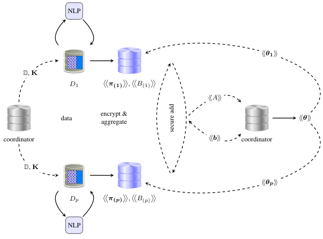
In Figure 3 we have outlined the encrypted pipeline, that combines Figure 1 with the inverse proposed in (Patrini et al., 2016), using Protocol 2: 2Classifier for Secure Text with Central Coordinator.

At each peer $p$ , we now wish to classify a particular observation vector ${\boldsymbol{x}}$ . Nominally, we would calculate

\hat{y}=\sign\left({\boldsymbol{\theta}}^{T}{\boldsymbol{x}}\right).

(19)

However, each peer only has a subset of features ${\boldsymbol{x}}_{[:]}$ . We note that the label is determined only by the sign of a scalar, and hence, we can break the inner product ${\boldsymbol{\theta}}^{T}{\boldsymbol{x}}$ into an inner product of local features and remote features as follows:

	$\displaystyle\hat{y}_{p}$	$\displaystyle=\sign\left({\boldsymbol{\theta}}_{\text{local}}^{T}{\boldsymbol{x}}_{\text{local}}+{\boldsymbol{\theta}}_{\text{remote}}^{T}{\boldsymbol{x}}_{\text{remote}}\right)$		(20)
		$\displaystyle=\sign\left(\underbrace{{\boldsymbol{\theta_{p}}}^{T}{\boldsymbol{x_{p}}}}_{\text{local}}+\underbrace{\sum_{q\neq p}{\boldsymbol{\theta_{q}}}^{T}{\boldsymbol{x_{q}}}}_{\text{remote}}\right).$		(21)

The local component of Equation (21) may be calculated at peer $p$ . If we denote the local classifier result as $\alpha_{p}$ , then we may write

$\displaystyle\alpha_{p}$	$\displaystyle={\boldsymbol{\theta_{p}}}^{T}{\boldsymbol{x_{p}}}\textrm{ and }$	(22)
$\displaystyle\hat{y}$	$\displaystyle=\sign\left(\sum_{p}\alpha_{p}\right)$	(23)
	$\displaystyle=\sign\left(\alpha_{p}+\sum_{q\neq p}\alpha_{q}\right)$	(24)

The summation in Equation (25) is the sum of all (local) calculated classifier results on the sub-components of the vector ${\boldsymbol{x}}$ . The result of Equation (25) shows that the remote classification results may be treated as offsets for the local result — that is, the remote inner products act as corrections to the local result. However, this requires that every peer share linking information about the observation ${\boldsymbol{x}}$ . To avoid this, we replace the summation in Equation (25) with an equivalent rado as follows:

\hat{y}=\sign\left(\alpha_{p}+{\boldsymbol{\theta_{\neg p}}}^{T}{\boldsymbol{\pi}}\right).

(25)

In the homomorphic encrypted case, the local inner product can be calculated by keeping the encrypted classifier vector ${\left\langle\!\left\langle{\boldsymbol{\theta}}\right\rangle\!\right\rangle}$ in its encrypted form, and treating the elements of ${\boldsymbol{x}}$ as unencrypted scalars. Finally, the summation may be achieved using multi-party secure addition, as outlined in (Clifton et al., 2002).

Protocol 3 Local Classify for Secure Text

0: coordinator

\mathcal{C}

with public-secret key pair

\mathbf{K}_{C},\mathbf{S}_{C}

0: common extra rado

{\left\langle\!\left\langle{\boldsymbol{\pi}}\right\rangle\!\right\rangle}

\mathcal{C}

0: binary feature vector

{\boldsymbol{f_{p}}}

\mathcal{C}

{ the features available at each peer

p

}

0: encrypted local classifier

{\left\langle\!\left\langle{\boldsymbol{\theta_{p}}}\right\rangle\!\right\rangle}

at each peer

p\in\{1,\ldots,P\}

\hat{y}

label from classification
at peer

p

{\left\langle\!\left\langle\alpha_{p}\right\rangle\!\right\rangle}\leftarrow

S.local.innerProd(

p,{\boldsymbol{x}},{\left\langle\!\left\langle{\boldsymbol{\theta_{p}}}\right\rangle\!\right\rangle}

) {Local.scalarproduct}
at each other peer

q\neq p

: {The set of peers may be chosen by

\mathcal{C}

}

{\left\langle\!\left\langle\alpha_{q}\right\rangle\!\right\rangle}\leftarrow

S.innerProd(

q,\mathcal{C},{\left\langle\!\left\langle{\boldsymbol{\pi}}\right\rangle\!\right\rangle},{\left\langle\!\left\langle{\boldsymbol{\theta_{q}}}\right\rangle\!\right\rangle}

) {Sec.innerproduct}
at peer

p

{\left\langle\!\left\langle\alpha\right\rangle\!\right\rangle}\leftarrow

SM.Add(

p=\{1,\ldots,P\},\{{\left\langle\!\left\langle\alpha_{p}\right\rangle\!\right\rangle}\}

) { using scalar

{\left\langle\!\left\langle\alpha_{p}\right\rangle\!\right\rangle}

}

send

{\left\langle\!\left\langle\alpha\right\rangle\!\right\rangle}

\mathcal{C}

\mathcal{C}

{\left\langle\!\left\langle\alpha\right\rangle\!\right\rangle}\stackrel{{\scriptstyle\text{decrypt}}}{{\longmapsto}}\alpha

send

s=\sign(\alpha)

to peer

p

p

\hat{y}\leftarrow s

Table 1: Results using numerical regression, and trivial text analytics. Encryption does not impact the accuracy of the results, but does dramatically reduce computation speed.

Grad descent algorithm	peers	rados	$\theta$	misclassification	run time (s)
LogisticRegression (baseline)	1	plain	plain	0.049	0.13s
radoBoost	1	plain	plain	0.12	1.4
radoLearn using rados from radoBoost	1	plain	plain	0.20	0.069
radoLearn	4	plain	plain	0.089	0.12
radoLearn	4	encrypted	plain	0.10	75
radoLearn	4	encrypted	encrypted	0.085	87

3.1 Usage Scenario for Multi-party, Private Text

In this scenario we outline the key procedure for learning from distributed private text corpora, and then classifying a locally private corpora. We shall use names to illuminate actors. Alice and Bob each have private text collections. Alice would like to classify her text by using a combination of patterns learnt from her own data and from Bob’s. Cate³³ 3 Cate plays no role in the learning, but is needed as a coordinator. provides coordination for Alice and Bob. Together, Alice, Bob and Cate follow Protocol 2 to establish a learned feature set. As Alice and Bob may have different feature sets, Cate separates Alice’s appropriate feature vector, and sets the remaining features to zero. Cate then coordinates Alice and Bob through Protocol 3.

4 Preliminary results

Using a simple data set from UCI Ionosphere data set – to provide a significant number of numeric features, agnostic of text input – we compare basic analytics using various privacy constraints. For comparison, (Zhou & Jiang, 2004) has reported a misclassification rate of 0.109, 0.112 & 0.096 using various neural network approaches. In our case, we have trialled standard linear regression, against multiple peers with rados, and $\theta$ all calculated in the encrypted domain. The results are shown in Table 1

Protocol 4 Secure Rado Solver

{\left\langle\!\left\langle T\right\rangle\!\right\rangle}\leftarrow

S.MatProd(

\left\{{\left\langle\!\left\langle B\right\rangle\!\right\rangle},{\left\langle\!\left\langle B\right\rangle\!\right\rangle}^{T}\right\}

) {Sec.mult}

{\left\langle\!\left\langle T\right\rangle\!\right\rangle}\leftarrow{\left\langle\!\left\langle T\right\rangle\!\right\rangle}\oplus\left[\mathrm{dim}_{c}(B)\otimes{\left\langle\!\left\langle\Gamma\right\rangle\!\right\rangle}\right]

{\left\langle\!\left\langle V\right\rangle\!\right\rangle}\leftarrow

S.Inv(

\left\{{\left\langle\!\left\langle T\right\rangle\!\right\rangle}\right\}

) {Sec.inversion }

{\left\langle\!\left\langle V\right\rangle\!\right\rangle}\leftarrow

S.MatProd(

\left\{{\left\langle\!\left\langle V\right\rangle\!\right\rangle},{\left\langle\!\left\langle B\right\rangle\!\right\rangle}\right\}

)

return First row of

{\left\langle\!\left\langle V\right\rangle\!\right\rangle}

5 Conclusion

We have outlined a protocol to provide secure text analytics, by combining standard features with numeric computation and secure linear algebra with obfuscated addition. Our result may also be used for numeric, un-trusted coordinators. Whilst not guaranteeing security, the protocol addresses common issues with sharing text data – namely visibility of identifiable information.

References

Carrell et al. (2013) Carrell, D, Malin, B, Aberdeen, J, Bayer, S, Clark, C, Wellner, B, and Hirschman, L. Hiding in plain sight: use of realistic surrogates to reduce exposure of protected health information in clinical text. Journal of the American Medical Informatics Association, 20(2):342–348, 2013.
Chazard et al. (2013) Chazard, E, Mouret, C, Ficheur, G, Schaffar, A, Beuscart, J B, and Beuscart, R. Proposal and evaluation of FASDIM, a Fast And Simple De-Identification Method for unstructured free-text clinical records. International Journal of Medical Informatics, 83(4):303–312, 2013.
Clifton et al. (2002) Clifton, Chris, Kantarcioglu, Murat, Vaidya, Jaideep, Lin, Xiaodong, and Zhu, Michael Y. Tools for privacy preserving distributed data mining. SIGKDD Explorations, 4(2), 2002.
Dalianis & Velupillai (2010) Dalianis, H and Velupillai, S. De-identifying Swedish clinical text — refinement of a gold standard and experiments with Conditional Random Fields. Journal of Biomedical Semantics, 1(1):6, 2010.
Damgård & Jurik (2001) Damgård, Ivan and Jurik, Mats. A generalisation, a simplification and some applications of Paillier’s probabilistic public-key system. In PKC ’01 Proceedings of the 4th International Workshop on Practice and Theory in Public Key Cryptography: Public Key Cryptography, pp. 119–136, 2001.
Dankar & Emam (2013) Dankar, Fida K. and Emam, Khaled El. Practicing differential privacy in health care: A review. Transactions on Data Privacy, 5:53–67, 2013.
Djatmiko et al. (2014) Djatmiko, Mentari, Friedman, Arik, Boreli, Roksana, Lawrence, Felix, Thorne, Brian, and Hardy, Stephen. Secure evaluation protocol for personalized medicine. In Workshop on Genome Privacy, 2014.
Djatmiko et al. (2016) Djatmiko, Mentari, Hardy, Stephen, Henecka, Wilko, Ott, Max, Smith, Guillaume, and Thorne, Brian. (confidential) N1Analytics: Distributed scoring with data confidentiality. whitepaper, January 2016.
Dunn et al. (2012) Dunn, Adam G., Day, Richard O., Mandl, Kenneth D., and Coiera, Enrico. Learning from hackers: Open-source clinical trials. Science, Translational Medicine, 4(132):132cm5, May 2012.
Dwork & Roth (2014) Dwork, Cynthia and Roth, Aaron. The algorithmic foundations of differential privacy. In Foundations and Trends in Theoretical Computer Science, volume 9, pp. 211–407. now, 2014.
Estrin & Sim (2010) Estrin, Deboarah and Sim, Ida. Open mhealth architecture: An engine for health care innovation. Science, 330(6005):759–760, November 2010.
Franz (2011) Franz, Martin. Secure Computations on Non-Integer Values. PhD thesis, Technische Universität Darmstadt, 2011.
From & Jakobsen (2006) From, Strange L. and Jakobsen, Thomas. Secure multi-party computation on integers. Master’s thesis, University of Aarhus, 2006.
Grouin & Neveol (2014) Grouin, C and Neveol, A. De-identification of clinical notes in French: towards a protocol for reference corpus development. Journal of Biomedical Informatics, 50:151–161, 2014.
Guo & Higham (2006) Guo, Chun-Hua and Higham, Nicholas J. A Schur-Newton method for the matrix $p$ ’th root and its inverse. Technical report, Manchester Institute for Mathematical Sciences, October 2006.
Hall et al. (2011 (revised 2013) Hall, Rob, Fienberg, Stephen E., and Nardi, Yuval. Secure multiple linear regression based on homomorphic encryption. Journal of Official Statistics, 27(4):669–691, 2011 (revised 2013).
Hirschberg & Manning (2015) Hirschberg, Julia and Manning, Christopher D. Advances in natural language processing. Science, 349(6245):261–266, July 2015.
Hrynaszkiewicz et al. (2010) Hrynaszkiewicz, Iain, Norton, Melissa L, Vickers, Andrew J, and Altman, Douglas G. Preparing raw clinical data for publication: guidance for journal editors, authors, and peer reviewers. British Medical Journal, 340, January 2010.
Ji et al. (2014) Ji, Zhanglong, Jiang, Xiaoqian, Wang, Shuang, Xiong, Li, and Ohno-Machado, Lucila. Differentially private distributed logistic regression using private and public data. BMC Medical Genomics, 7:S14, 2014.
Jin (2007) Jin, Huidong (Warren). Practical issues on privacy-preserving health data mining. In Working Notes of PAKDD’07 Industrial Track, 2007.
Johnson (2014) Johnson, Mark. Beyond the 1-best pipeline. Presentation slides, at NICTA-NLP workshop 2014, September 2014.
Kayaalp et al. (2014) Kayaalp, M, Browne, A C, Callaghan, F M, Dodd, Z A, Divita, G, Ozturk, S, and McDonald, C J. The pattern of name tokens in narrative clinical text and a comparison of five systems for redacting them. Journal of the American Medical Informatics Association, 21(3):423–431, 2014.
McDonald & Kelly (2012) McDonald, Diane and Kelly, Ursula. The value and benefit of text mining to UK further and higher education. Digital infrastructure. available online http://bit.ly/jisc-textm, 2012.
McKeon et al. (2013) McKeon, Simon, Alexander, Elizabeth, Brodaty, Henry, Ferris, Bill, Frazer, Ian, and Little, Melissa. Strategic review of health and medical research – better health through research. Technical report, Australian Government, Department of Health and Ageing, April 2013.
Meystre et al. (2014) Meystre, S M, Ferrández, Ó, Friedlin, F J, South, B R, Shen, S, and Samore, M H. Text de-identification for privacy protection: A study of its impact on clinical text information content. Journal of Biomedical Informatics, 50(Supplement C):142–150, 2014. Special Issue on Informatics Methods in Medical Privacy.
Morita et al. (2013) Morita, M, Kano, Y, Ohkuma, T, Miyabe, M, and Aramaki, E. Overview of the NTCIR-10 MedNLP task. In Proceedings of the 10th NTCIR Conference, Tokyo, Japan, 2013. NTCIR.
Nock et al. (2015) Nock, Richard, Patrini, Giorgio, and Friedman, Arik. Rademacher observations, private data, and boosting. J Machine Learning Research, 37, 2015.
Oard (2015) Oard, Douglas. Keynote presentation: Beyond information retrieval: When and how not to find things. In CLEF, 2015.
Pahikkala et al. (2012) Pahikkala, T., Suominen, Hanna Jasmine, and Boberg, J. Efficient cross-validation for kernelized least-squares regression with sparse basis expansions. Machine Learning, 87(3):381–407, 2012.
Paillier (1999) Paillier, Pascal. Public-key cryptosystems based on composite degree residuosity classes. In EUROCRYPT, pp. 223–238. Springer-Verlag, 1999.
Patrini et al. (2016) Patrini, Giorgio, Nock, Richard, Hardy, Stephen, and Caetano, Tiberio. Fast learning from distributed datasets without entity matching. Technical report, Data61, March 2016.
Paverd et al. (2014) Paverd, Andrew, Martin, Andrew, and Brown, Ian. Modelling and automatically analysing privacy properties for honest-but-curious adversaries. Tech. Report, 2014.
Rajagopalan (1996) Rajagopalan, Jayasiree. An Iterative Algorithm for Inversion of Matrices. PhD thesis, Concordia University, Montreal, Canada, September 1996.
Sayogo & Pardo (2012) Sayogo, Djoko Sigit and Pardo, Theresa A. Exploring the motive for data publication in open data initiative: Linking intention to action. In System Science (HICSS), pp. 2623–2632, Hawaii, USA, January 2012.
Shannon (1949) Shannon, Claude E. Communication theory of secrecy systems. The Bell System Technical Journal, 28(4):656–715, May 1949.
Shaw et al. (2016) Shaw, D M, Gross, J V, and Erren, T C. Data donation after death: A proposal to prevent the waste of medical research data. EMBO Reports, 17(1):14–17, 2016.
Si et al. (2014) Si, Luo, Yang, Grace Hui, Zhang, Sicong, and Cen, Lei (eds.). Proceeding of the 1st International Workshop on Privacy-Preserving IR: When Information Retrieval Meets Privacy and Security, 2014.
Simon et al. (2009) Simon, R S, Evans, S J, Benjamin, A, Delano, D, and Bates, W D. Patients’ attitudes toward electronic health information exchange: Qualitative study. Journal of Medical Internet Research, 11, 2009.
Soleymani (2012) Soleymani, Fazlollah. A rapid numerical algorithm to compute matrix inversion. International Journal of Mathematics and Mathematical Sciences, 2012, 2012.
Stenetorp et al. (2012) Stenetorp, Pontus, Pyysalo, Sampo, Topić, Goran, Ohta, Tomoko, Ananiadou, Sophia, and Tsujii, Jun’ichi. brat: a web-based tool for nlp-assisted text annotation. In Proceedings of the Demonstrations Session at EACL, 2012.
Suominen et al. (2014) Suominen, Hanna, Johnson, Maree, Zhou, Liyuan, Sanchez, Paula, Sirel, Raul, Basilakis, Jim, Hanlen, Leif, Estival, Dominique, Dawson, Linda, and Kelly, Barbara. Capturing patient information at nursing shift changes: methodological evaluation of speech recognition and information extraction. J. Am. Med. Info. Assoc., October 2014.
Suominen et al. (2008) Suominen, Hanna J., Pahikkala, T., and Salakoski, Tapio. Critical points in assessing learning performance via cross-validation. In Proceedings of the 2nd International and Interdisciplinary Conference on Adaptive Knowledge Representation and Reasoning (AKRR 2008), pp. 9–22, 2008.
Suominen et al. (2015) Suominen, Hanna J., Zhou, Liyuan, Hanlen, Leif W., and Ferraro, Gabriela. Benchmarking clinical speech recognition and information extraction: New data, methods, and evaluations. JMIR Med Inform, 2(3), April 2015.
Sweeney (2015) Sweeney, L. Only you, your doctor, and many others may know. Technology Science, 2015092903, 2015.
Thomson (2004) Thomson, Colin. The regulation of health information privacy in Australia. Technical report, National Health and Medical Research Council, 2004.
Veitch & Barbour (2010) Veitch, Emma and Barbour, Virginia. Innovations for global health equity: beyond open access towards open data. MEDICC Rev, 12(3):48, Jul 2010.
Verhulst et al. (2014) Verhulst, Stefaan, Noveck, Beth Simone, Caplan, Robyn, Brown, Kristy, and Paz, Claudia. The open data era in health and social care: A blueprint for the National Health Service (NHS England) to develop a research and learning programme for the open data era in health and social care. online http://images.thegovlab.org/wordpress/wp-content/uploads/2014/06/nhs-full-report.pdf, May 2014.
Vogel (2011) Vogel, Lauren. The secret’s in: open data is a foreign concept in Canada. Canadian Medical Association Journal, 183(7):E375–6, Apr 2011. doi: 10.1503/cmaj.109-3837.
Yu et al. (2011) Yu, Ching-Hua, Chow, Sherman S. M., Chung, Kai-Min, and Liu, Feng-Hao. Efficient secure two-party exponentiation. In CT-RSA, pp. 17–32, San Francisco, CA, February 2011.
Zhou & Jiang (2004) Zhou, Zhi-Hua and Jiang, Yuan. NeC4.5: Neural ensemble based C4.5. IEEE Transactions on Knowledge and Data Engineering, June 2004.