Smoothed SVD-based Beamforming for FBMC/OQAM Systems Based on Frequency Spreading

Fig. 1 presents the equivalent baseband block diagram of an FBMC/OQAM system. It consists of $M$ subcarriers with subcarrier spacing $1/T$, where $T$ is the interval between the complex-valued symbols in time. Each complex-valued symbol is partitioned into a pair of real-valued PAM symbols. The PAM symbol at the frequency-time index $(m,n)$ is denoted by $a_{m,n}$, where $m$ is the frequency/subchannel index and $n$ is the time index. Moreover, $a_{m,2\hat{n}}$ and $a_{m,2\hat{n}+1}$, with integer $\hat{n}$, are real and imaginary parts of a QAM symbol and are $T/2$ spaced in time. With a sampling interval of $T/M$, the filter bank prototype filter has the discrete time impulse response $g(i)$, which we assume only have non-zero coefficients for $0<i\leq KM-1$, where $K$ is a positive integer. We further assume that $g(i)$ is an even-symmetric pulse, i.e., $g(i)=g(KM-i)$.

The discrete-time baseband equivalent of an FBMC/OQAM signal may be presented as [42, 2]

where $g_{m,n}(i)$ is the pulse of the $(m,n)$-th PAM symbol. When an FBMC/OQAM signal is transmitted through a channel that varies slowly with time and its delay spread is significantly shorter than the symbol interval, the channel transfer function over each subchannel may be approximated by a flat gain. Let $H_{m,n}$ denote this gain for the $m$-th subchannel at the $n$-th time index. With the slow varying assumption, we omit the subscript $n$ from $H_{m,n}$ for simplicity of presentation. Then, the $m_{0}$th output of the receiver analysis filter bank at the $n_{0}$th time index is obtained as, [42, 2],

where

It is noteworthy that for a well-designed prototype filter $g(i)$, ${\zeta_{m,n}^{m_{0},n_{0}}=1}$ when $(m,n)=(m_{0},n_{0})$, and is zero or a pure imaginary value when $(m,n)\neq(m_{0},n_{0})$, e.g., see [1]. To be more specific, ${\zeta_{m,n}^{m_{0},n_{0}}}$, for $(m,n)\neq(m_{0},n_{0})$, represents the imaginary interference to $a_{m,n}$, which could be removed by taking the real part after channel equalization.

We consider a MIMO system equipped with ${N_{\textrm{t}}}$ transmit antennas and ${N_{\textrm{r}}}$ receive antennas, which supports ${L}$ parallel streams. The SVD decomposition of the channel ${\bf{H}}\in{\mathbb{C}^{{N_{\textrm{r}}}\times{N_{\textrm{t}}}}}$ is:

where ${\bf{V}}\in{\mathbb{C}^{{N_{\textrm{t}}}\times{N_{\textrm{t}}}}}$ and ${\bf{U}}\in{\mathbb{C}^{{N_{\textrm{r}}}\times{N_{\textrm{r}}}}}$ are unitary matrices, and ${\bf{D}}$ is an $N_{\textrm{r}}$-by-$N_{\textrm{t}}$ rectangular diagonal matrix containing $(\lambda^{1},\lambda^{2}\ldots)$ as diagonal elements, where $\lambda^{1},\lambda^{2}\ldots$ denote the singular values that are sorted in descending order and are real-valued. When ${L=N_{\textrm{t}}=N_{\textrm{r}}}$, the transmit beamformer and receive beamformer are simply ${\bf{V}}$ and ${\bf{U}}^{\textrm{H}}$, respectively. When $L<N_{\textrm{t}}$ or $L<N_{\textrm{r}}$, they are submatrices of $\bf{V}$ and ${\bf{U}}^{\textrm{H}}$, respectively, corresponding to the $L$ largest singular values. For clarity of notations, we abuse the notations $\bf{V}$ and/or ${\bf{U}}^{\textrm{H}}$ and let them also represent the beamformers when $L<N_{\textrm{t}}$ or $L<N_{\textrm{r}}$ in the rest of this paper, then ${\bf{V}}\in{\mathbb{C}^{{N_{\textrm{t}}}\times{L}}}$ and ${\bf{U}}^{\textrm{H}}\in{\mathbb{C}^{{L}\times{N_{\textrm{r}}}}}$. With the transmit beamforming and MIMO channel, the signal at the receiver is

where $\bf{s}$ is the symbols to be transmitted and $\bf{n}$ is the receive noise vector ($\bf{y}$, $\bf{s}$ and $\bf{n}$ are ${N_{\textrm{r}}}\times{1}$, ${L}\times{1}$ and ${N_{\textrm{r}}}\times{1}$ vectors, respectively). The signal after receive beamforming is

where $\widetilde{\bf{n}}={\bf{U}}^{\textrm{H}}{\bf{n}}$ ($\bf{r}$ and $\widetilde{\bf{n}}$ are ${L}\times{1}$ vectors). Clearly, the transmitted symbols are recovered with nonequal gains [43], and there is no interference among streams.

In this subsection, we present the model of straightforward combination of SVD and FBMC/OQAM and discuss about the interference leakage problem. Combining the models in subsection II-A and II-B, the transmitted signal of the SVD-FBMC/OQAM is represented by a sequence of vectors ${\bf{x}}(i)=[{x_{1}}(i)~{x_{2}}(i)\cdot\cdot\cdot{x_{N_{\textrm{t}}}}(i)]^{\textrm{T}}$ as

where ${\bf{a}}_{m,n}=[a_{m,n}^{1}~a_{m,n}^{2}\cdot\cdot\cdot a_{m,n}^{L}]^{\textrm{T}}$ is the symbol vector to be transmitted, and ${g_{m,n}}(i)$ is the frequency-time shifted version of prototype filter $g(i)$ (see (1)), ${{\bf{V}}_{m}}\in{\mathbb{C}^{{N_{\textrm{t}}}\times{L}}}$ denotes the beamforming matrix for the $m$-th subchannel. Assuming nearly flat fading across the subcarrier band (the bandwidth of subchannel), the received signal at the output of analysis filters for Time $n_{0}$ and Subchannel $m_{0}$ is

where ${{\bf{H}}_{m}}\in{\mathbb{C}^{{N_{\textrm{r}}}\times{N_{\textrm{t}}}}}$ is the MIMO channel response of Subchannel $m$, ${\bf{U}}_{m_{0}}^{\textrm{H}}\in{\mathbb{C}^{{L}\times{N_{\textrm{r}}}}}$ is the receive beamformer for the $m_{0}$-th subchannel. Clearly, the first term of (8) is the recovered symbols and the second term is the ICI/ISI interference. If ${\bf{H}}_{{m_{0}}}\approx{\bf{H}}_{{m}}$ and ${\bf{V}}_{{m_{0}}}\approx{\bf{V}}_{{m}}$ for subchannels adjacent to $m_{0}$, we have ${{\bf{U}}_{{m_{0}}}^{\textrm{H}}{{\bf{H}}_{m}}{{\bf{V}}_{m}}}\approx{{\bf{D}}_{m_{0}}}$, and the ISI/ICI term is approximately imaginary and could be removed by taking the real part of ${{\bf{r}}_{{m_{0}},{n_{0}}}}$ (recall that ${{\bf{D}}_{m_{0}}}$ is real-valued). However, this does not work even under channels with moderate frequency selectivity. The reason is that: the transmit and receive beamformer may experience significant changes between adjacent subchannels due to channel variation, then ${{\bf{U}}_{{m_{0}}}^{\textrm{H}}{{\bf{H}}_{m}}{{\bf{V}}_{m}}}$ is not real-valued and the ISI/ICI term is no longer pure imaginary, which results in leaked ICI/ISI interference into the real part of ${{\bf{r}}_{{m_{0}},{n_{0}}}}$.

The FS-FBMC structure, a special form of the fast convolution implementation of filter banks [44, 45, 46, 47, 48, 49], uses frequency spreading/despreading to implement the filtering in the frequency domain for FBMC/OQAM systems. In FS-FBMC, FFT/IFFT is taken at the length of $KM$. Let $G(k)$ denote the FFT of a segment of $g(i)$ in the range of $0\leq i\leq{KM-1}$, where $0\leq k\leq{KM-1}$ is the index of FS-FBMC tones. We assume that $G(k)$ has $2P-1$ non-negligible tones that center around the zero-th tone, where $P$ is a positive integer. Let $G_{m,n}^{(n_{0})}(k)$ denote the FFT of a segment of $g_{m,n}(i)$ in the range of $n_{0}M/2\leq i\leq{n_{0}M/2+KM-1}$, which is the portion of $g_{m,n}(i)$ that falls inside the $n_{0}$-th sliding window. The superscript $(n_{0})$ is to emphasize that the FFT is taken at the $n_{0}$-th window. Then, the filtering at the $n$-th time index is implemented in the frequency domain by spreading the PAM symbols with $G_{m,n}^{(n)}(k)$ as

where $G_{m,n}^{(n)}(k)$ is the FFT of the non-zero part of pulse $g_{m,n}(i)$, i.e., at the $n$-th window. And, the output of the frequency spreading is fed to the IFFT transformation to obtain the time domain samples of the $n$-th time index as

Then, the transmitted time sequence is obtained by accumulation over all symbols as

At the receiver, a sliding window is employed to select $KM$ samples every $M/2$ samples, which are fed to an FFT module. Then, the transmitted PAM symbols are recovered through equalization and frequency despreading. More details of FS-FBMC transmission could be found in [50].

Fig. 2 presents the transmitter of the proposed finer SVD-FS-FBMC, where ${\bf{V}}_{k}\in{\mathbb{C}^{{N_{\textrm{t}}}\times{L}}}$ is the beamforming matrix for the $k$-th FS-FBMC tone, and ${\bf{V}}_{k}=[{\bf{v}}_{k}^{1}~{\bf{v}}_{k}^{2}\cdot\cdot\cdot{\bf{v}}_{k}^{L}]$, here ${\bf{v}}_{k}^{l}$ denotes the beamforming vector for the $l$-th stream. The beamformed signals on all transmit antennas for the $k$-th tone and $n$-th time index is given by an $N_{\textrm{t}}$-by-1 vector

Then, the samples on all transmit antennas for the $n$-th time index is obtained by IFFT

where ${\bf{x}}_{n}(i)$ is an $N_{\textrm{t}}$-by-$1$ vector.

After accumulation over all symbols, the transmitted signals on all antennas are represented by the following vector sequence

Fig. 3 presents the receiver of the proposed SVD-FS-FBMC, where ${\bf{U}}^{\textrm{H}}_{k}\in{\mathbb{C}^{{L}\times{N_{\textrm{r}}}}}$ is the beamforming matrix for the $k$-th FS-FBMC tone, and ${\bf{U}}_{k}^{\textrm{H}}=[({\bf{u}}_{k}^{1})^{\textrm{H}}~({\bf{u}}_{k}^{2})^{\textrm{H}}\cdot\cdot\cdot({\bf{u}}_{k}^{L})^{\textrm{H}}]$, here $({\bf{u}}_{k}^{l})^{\textrm{H}}$ denotes the receive beamforming vector for the $l$-th stream. Let $N_{\textrm{r}}$-by-1 vector ${\bf{y}}(i)$ denote the $i$-th received samples on all receive antennas, and ${\bf{y}}^{(n_{0})}(i)$ ($0\leq i\leq{KM-1}$) denote the selected $KM$ samples by the $n_{0}$-th sliding window, i.e., ${\bf{y}}^{(n_{0})}(i)={\bf{y}}(i+n_{0}M/2)$, for $0\leq i\leq KM-1$. Taking FFT of ${\bf{y}}^{(n_{0})}(i)$, we obtain

Applying the receive beamformer, we have the signals received on the $k$-th tone

where $\widetilde{{\bf{s}}}^{(n_{0})}(k)$ is an $L$-by-$1$ vector that holds the samples of all streams. Noting that different tones and streams may have different singular values, an equalizer is required at each tone for each stream. The equalizers for the $k$-th tone is represented by an $L$-by-$L$ diagonal matrix ${\bf{E}}_{k}={\rm{diag}}\left\{E_{k}^{1},E_{k}^{2},\ldots,E_{k}^{L}\right\}$, where $E_{k}^{l}$ is the equalizer for Stream $l$ and Tone $k$. If it is a zero forcing (ZF) equalization, $E_{k}^{l}=1/\lambda_{k}^{l}$. Then, the equalized signal is obtained as

Finally, despreading is applied to obtain the PAM symbols at the $m_{0}$-th subchannel and $n_{0}$-th time index

Under the assumption that ${\bf{E}}_{k}$, ${\bf{U}}_{k}$, ${\bf{H}}_{k}$ and ${\bf{V}}_{k}$ are nearly flat, i.e., they vary slowly, across the subcarrier band,

where ${\bf{n}}^{(n_{0})}(k)$ is FFT of the noise with ${\bf{y}}^{(n_{0})}(i)$. Proof of this equation is presented in the Appendix. Clearly, the first term of (19) is the transmitted PAM symbols, and the second term is the ICI/ISI interference that is pure imaginary under the nearly-flat assumption and could be removed by taking the real part.

Obviously, the complexity of beamforming in the proposed SVD-FS-FBMC system is roughly proportional to the number of tones per subchannel, i.e. $K$. When $K=1$, i.e. without frequency spreading and despreading, the proposed SVD-FS-FBMC is exactly the same as that of SVD-OFDM with the same subchannel number $M$. Therefore, the complexity of beamforming in the proposed SVD-FS-FBMC is $K$ times that of the SVD-OFDM with the same subchannel number $M$.

Compared with the straightforward SVD-FBMC/OQAM given in Section II-C, the major improvement by the finer beamforming is that it allows smoother transition of beamformers.

To deal with this problem, we propose in this subsection a smoothing criterion and method to smooth the output of any given SVD algorithm so that it satisfies the nearly-flat requirement. The idea here is as follows: We smooth the output of the given SVD algorithm, denoted by ${\hat{\bf{V}}}_{k}$, to obtain ${\bf{V}}_{k}$ such that its Euclidean distance to ${\bf{V}}_{k-1}$ is bounded as given in Section IV. The criterion of minimizing the distance of adjacent beamformers is intuitive, due to the fact that Euclidean distance, i.e., Euclidean difference of adjacent vectors, is a measure of first-order smoothness for vector functions. In addition, the criterion is known to be effective thanks to the discussion in Section IV. Running this operation from the beginning to the end of the active frequency tones, a sequence of smoothed beamformers is obtained. It is worth mentioning here that we have also attempted to optimize the second-order smoothness, however no further observable gain over the first-order smoothness optimization was obtained. The reason is that the channel frequency response is rather smooth with the finer beamforming and second-order smoothness or above is unnecessary, under the system parameters and channel models considered in Section VI.

It is assumed that ${\hat{\bf{v}}_{k}^{l}}$ is the $l$-th right singular vector given by the SVD algorithm, corresponding to the singular value ${\hat{\lambda}_{k}^{l}}$ of ${{\bf{H}}_{k}}$, here the hat $\hat{~}$ is to emphasize that ${\hat{\bf{v}}_{k}^{l}}$ and ${\hat{\lambda}_{k}^{l}}$ are the outputs of the SVD algorithm before smoothing. Taking ${\hat{\bf{v}}_{k}^{l}}$ as the input, after smoothing, ${{\bf{v}}_{k}^{l}}$ is output as the beamformer.

The subspace spanned by ${\hat{\bf{v}}_{k}^{l}}$ can be represented by a set ${\bf\Pi}(\hat{{\bf{v}}}_{k}^{l})=\{\beta{\hat{\bf{v}}_{k}^{l}}{e^{j\theta}}|\beta\in\mathbb{R},\theta\in[0,2\pi)\}$. If ${\hat{\lambda}_{k}^{l}}$ satisfy the separation conditions, distance from ${\bf\Pi}(\hat{{\bf{v}}}_{k}^{l})$ to ${\bf\Pi}({{\bf{v}}}_{k-1}^{l})$ is bounded due to the Wedin theorem, here ${{\bf{v}}}_{k-1}^{l}$ is the smoothed beamformer of the $(k-1)$-th frequency tone. Therefore, a vector that has a bounded Euclidean distance to ${{\bf{v}}}_{k-1}^{l}$ is available in ${\bf\Pi}(\hat{{\bf{v}}}_{k}^{l})$. Then, the problem of smoothing the SVD output is solved by

where ${e^{j\theta^{*}}}$ is a phase factor that minimizes the distance from ${e^{j\theta}}{\hat{\bf{v}}_{k}^{l}}$ to ${\bf{v}}_{k-1}^{l}$, i.e.,

The solution to the phase factor optimization problem is

Combining (27) and (29), we have the smoothed output as

When two singular values become very close to each other, the bound given by the Wedin theorem is not close to zero even when the channel frequency response is smooth, then smoothness between adjacent beamformers cannot be guaranteed. Still, smoothing is needed to minimize the Euclidian distance of ${\bf{v}}_{k}^{l}$ and ${\bf{v}}_{k-1}^{l}$ for all $l$’s. While smoothing the SVD output in this case, a special problem needs to be treated carefully. The problem is the ambiguity in pairing one from $\{\hat{\bf{v}}_{k}^{l},\ldots,\hat{\bf{v}}_{k}^{L}\}$ with ${\bf{v}}_{k-1}^{l}$, which is explained in the following. When $\hat{\lambda}_{k}^{l}\approx\lambda_{k-1}^{l}$ and it is separated from other singular values, there is no doubt that $\hat{\bf{v}}_{k}^{l}$ should be paired with ${\bf{v}}_{k-1}^{l}$. However, when there are multiple singular values of the $k$-th frequency tone approximate $\lambda_{k-1}^{l}$, i.e., $\hat{\lambda}_{k}^{l_{1}}\approx\ldots\approx\hat{\lambda}_{k}^{l_{m}}\approx\lambda_{k-1}^{l}$, where $m$ is the number of singular values that are close to $\lambda_{k-1}^{l}$, there has to be a method to determine which of $\hat{\lambda}_{k}^{l_{1}},\ldots,\hat{\lambda}_{k}^{l_{m}}$ ($\hat{\bf{v}}_{k}^{l_{1}},\ldots,\hat{\bf{v}}_{k}^{l_{m}}$) should be paired with $\lambda_{k-1}^{l}$ (${\bf{v}}_{k-1}^{l}$), i.e., which one belongs to the $l$-th stream.

To resolve this ambiguity, we measure the subspace distance from $\hat{{\bf{v}}}_{k}^{l_{i}}$ to ${{\bf{v}}}_{k-1}^{l}$, for ${l_{1},\ldots,l_{m}}$, and select the one with the minimum subspace distance to pair with ${{\bf{v}}}_{k-1}^{l}$. The subspace distance of two vectors, ${\hat{\bf{v}}_{k}^{{l_{i}}}}$ and ${\hat{\bf{v}}_{k-1}^{{l}}}$ in our discussion, is defined as [51]

and let

Then, $\hat{\lambda}_{k}^{l_{*}}$ is taken as the singular value of Stream $l$, and ${{\hat{\bf{v}}}_{k}^{{l_{*}}}}$ is smoothed to generate the beamformer as

In this subsection, we introduce the orthogonal iteration method [51] for smoothing, which spontaneously follows the proposed smoothing criterion due to its iterative nature. Compared with the phase factor optimization method, the orthogonal iteration enjoys lower computational complexity. The orthogonal iteration method has been used in [52] to provide smooth beamforming for an OFDM system to enable channel state information (CSI) smoothing.

As we know, ${\bf{V}}_{k}$ is the right singular vectors of ${\bf{H}}_{k}$, as well as the eigenvectors of ${\bf{A}}_{k}={\bf{H}}_{k}^{\textrm{H}}{\bf{H}}_{k}$, which can be found by performing the following iteration from an initial matrix ${{\bf{Q}}^{(0)}}\in{\mathbb{C}^{{N_{\textrm{t}}}\times{L}}}$ with orthonormal columns

where $i$ denotes the iteration index and $N_{\rm{iter}}$ is the total number of iterations. According to [52], ${{\bf{R}}^{(i)}}$ converges to a diagonal matrix containing the eigenvalues of ${{\bf{A}}_{k}}$, and ${{\bf{Q}}^{(i)}}$ converges to an orthonormal basis for the dominant subspace of dimension $L$.

For a beamforming that is smooth from Tone $k-1$ to $k$, ${\bf{V}}_{k-1}$ could serve as the initial ${{\bf{Q}}^{(0)}}$, and the output is ${\bf{V}}_{k}={{\bf{Q}}^{(N_{\rm{iter}})}}$. It will be shown in the next section that very few iterations are needed to obtain a satisfactory ${\bf{V}}_{k}$, which ensures smoothness from ${\bf{V}}_{k-1}$ to ${\bf{V}}_{k}$. The complete algorithm is presented in Algorithm 1.

Let us first check if the smoothness across tones is improved with the proposed smoothing methods introduced in Section V. Smoothness between two beamformers of adjacent tones is measured by their Euclidean difference. Fig. 4 presents the histogram of the Euclidean distance between adjacent beamformers by the proposed methods. Result by the SVD function in the Matlab software is also presented for comparison. The distance of the proposed schemes falls in the range of $0\sim 1.0$, while that of SVD Matlab could go beyond $1.0$ with non-negligible percentage. It is thus concluded that the phase factor optimization and the orthogonal iteration method provide significant smoothness improvements compared with the SVD of no smoothness consideration. It is also observed that there is no observable difference in the histogram between the phase factor optimization and orthogonal iteration with $N_{\rm{iter}}=3$, which verifies the ability of the orthogonal iteration to fulfill the proposed smoothing criterion spontaneously.

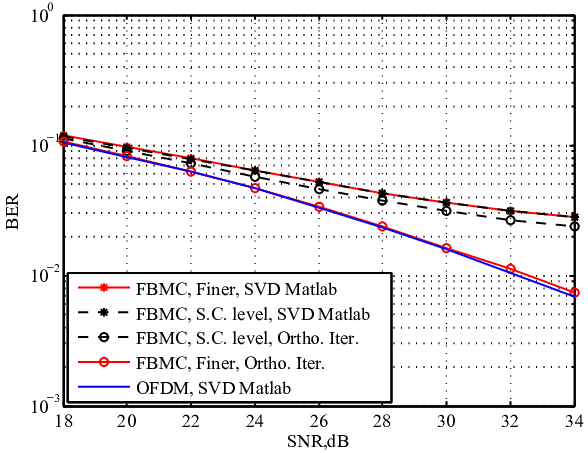
The simulation results in this subsection mainly demonstrate the performance of the orthogonal iteration method, the comparison between the orthogonal iteration method and the phase factor optimization method is presented in Subsection VI-C. Fig. 5 and 6 present BER performance of the SVD-FS-FBMC system with the proposed finer beamforming and smoothing under Channel Model D, without and with coding, respectively. For comparison, we also present BER results of the following four systems: i) SVD-OFDM; ii) Basic SVD-FBMC/OQAM with subchannel-level (S.C. level) beamforming and without smoothing (SVD Matlab), this is the straightforward combination of SVD and FBMC/OQAM discussed in Section II; iii) SVD-FBMC/OQAM with subchannel-level beamforming and smoothing (orthogonal iteration), its performance gap to the proposed SVD-FS-FBMC shows how the proposed beamforming with finer granularity improves the performance; iv) SVD-FS-FBMC with the finer beamforming but without smoothing (SVD Matlab), its performance gap to the proposed SVD-FS-FBMC shows how the proposed smoothing improves the performance. The schemes under comparison are summarized in Table II. The simulations of Fig. 5 and 6 demonstrate that both beamforming with finer granularity and smoothing are necessary for a good beamforming of FBMC system under frequency selective channels. The results clearly show that the SVD-FS-FBMC system with the proposed finer beamforming and smoothing greatly outperforms the other SVD-FBMC/OQAM and SVD-FS-FBMC systems. And it performs very closely with SVD-OFDM, in terms of BER, under the IEEE 802.11n Channel Model D. It is also observed that smoothing is crucial for the BER performance: the subchannel-level SVD-FBMC/OQAM systems with smoothing outperforms the SVD-FBMC/OQAM without smoothing. One may notice that the system with finer beamforming but no smoothing has the worst BER performance among the systems in comparison. The reason is that, when finer beamforming is employed without smoothing, significant changes of beamformer may happen between two tones of one subcarrier band, which results in serious distortion of the transmitted signal.

Performance of the proposed scheme is also evaluated under channels of more frequency selectivity, i.e., Channel Model E and F, with $2/3$ coding, for $64$-QAM and $16$-QAM modulation, respectively in Fig. 7 and Fig. 8. As the channel selectivity increases, error floor is observed for FBMC systems. Employing lower-order modulation reduces the performance gap between the proposed SVD-FS-FBMC and SVD-OFDM, however does not stop it from growing at high SNRs under the Channel Model F.

In the simulation of Fig. 9, we increase the FFT size to $8M$ and test the proposed SVD-FS-FBMC under channel Model F. Increasing the FFT size from $4M$ to $8M$ doubles the number of frequency tones of the FS-FBMC receiver, and therefore gives even finer beamforming, at the cost of doubled complexity. As observed from Fig. 9, performance of the proposed SVD-FS-FBMC is improved at high SNRs and close to that of SVD-OFDM.

It should be noted that the BER plots above is with respect to SNR. If we use $E_{b}/N_{0}$ instead of SNR for x-axis, about 1 dB gain of the proposed SVD-FS-FBMC will be observed over SVD-OFDM, because that the SVD-FS-FBMC does not pay for the energy overhead to transmit the 25% cyclic prefix as the OFDM in IEEE 802.11n does.

In this subsection, we examine the number of iterations required for the smoothing of orthogonal iteration and then give a complexity comparison between the phase factor optimization and orthogonal iteration.

The BER performance of the proposed SVD-FS-FBMC system with orthogonal iteration is presented for different number of iterations in Fig. 10, with $2/3$ coding, $64$-QAM modulation, various channel models. Performance of phase factor optimization is also presented for comparison. As observed from Fig. 10, $N_{\rm{iter}}=3$ is adequate for the orthogonal iteration method to achieve a similar performance as the phase factor optimization under Channel Model D, E and F. For channel model with less frequency selectivity, such as Channel Model D and E, the number of iterations could be further reduced.

We express the computational complexity in terms of the number of floating point operations (FLOPS) [57]. Each scalar/complex addition or multiplication is counted as one FLOPS. Table III shows the complexity of operations in smoothed SVD with orthogonal iteration [57]. Assuming $N_{\rm{iter}}=3$ and ${N_{t}}={N_{r}}$, the total complexity of the orthogonal iteration for each frequency tone is $13N_{t}^{3}-\frac{5}{2}N_{t}^{2}-\frac{1}{2}{N_{t}}$ FLOPS. Omitting the small order terms, the complexity is $13N_{t}^{3}$ FLOPS for each frequency tone. For the phase factor optimization method, the major complexity of each frequency tone is the direct computation of SVD from the channel matrix ${{\bf{H}}_{k}}$, which is about $4N_{t}^{2}N_{r}+8N_{t}N_{r}^{2}+9N_{r}^{3}$ FLOPS as given in [58]. Assuming ${N_{t}}={N_{r}}$, the complexity of the phase factor optimization is $21N_{t}^{3}$ FLOPS for each frequency tone, which is higher than that of the orthogonal iteration with three iterations.

References

- [1] B. Farhang-Boroujeny, “OFDM versus filter bank multicarrier,” IEEE Signal Processing Magazine, vol. 28, no. 3, pp. 92-112, May 2011.
- [2] P. Siohan, C. Siclet, and N. Lacaille, “Analysis and design of OQAM/OFDM systems based on filterbank theory,” IEEE Transactions on Signal Processing, vol. 50, no. 5, pp. 1170-1183, May 2002.
- [3] B. Hirosaki, “An orthogonally multiplexed QAM system using the discrete Fourier transform,” IEEE Transactions on Communications, vol. 29, no. 7, pp. 982-989, Jul. 1981.
- [4] T. Ihalainen, A. Ikhlef, J. Louveaux, and M. Renfors, “Channel Equalization for Multi-Antenna FBMC/OQAM Receivers,” IEEE Transactions on Vehicular Technology, vol. 60, no. 5, pp. 2070-2085, Jun. 2011.
- [5] X. Gao, W. Wang, X. Xia, E. K. S. Au, and X. You, “Cyclic prefixed OQAM-OFDM and its application to single-carrier FDMA,” IEEE Transactions on Communications, vol. 59, no. 5, pp. 1467-1480, May 2011.
- [6] D. Chen, D. Qu, T. Jiang, and Y. He, “Prototype filter optimization to minimize stopband energy with NPR constraint for filter bank multicarrier modulation systems,” IEEE Transactions on Signal Processing, vol. 61, no. 1, pp. 159-169, Jan. 2013.
- [7] H. Zhang, D. Le Ruyet, D. Roviras, and H. Sun, “Noncooperative multicell resource allocation of FBMC-based cognitive radio systems,” IEEE Transactions on Vehicular Technology, vol. 61, no. 2, pp. 799-811, Feb. 2012.
- [8] W. Wang, X. Gao, F. Zheng, and W. Zhong, “CP-OQAM-OFDM based SC-FDMA: adjustable user bandwidth and space-time coding,” IEEE Transactions on Wireless Communications, vol. 12, no. 9, pp. 4506-4517, Sep. 2013.
- [9] D. Qu, S. Lu, and T. Jiang, “Multi-block joint optimization for the peak-to-average power ratio reduction of FBMC-OQAM signals,” IEEE Transactions on Signal Processing, vol. 61, no. 7, pp. 1605-1613, Apr. 2013.
- [10] W. Cui, D. Qu, T. Jiang, and B. Farhang-Boroujeny, “Coded auxiliary pilots for channel estimation in FBMC-OQAM systems,” IEEE Transactions on Vehicular Technology, vol. 65, no. 5, pp. 2936-2946, May 2016.
- [11] L. Zhang, P. Xiao, A. Zafar, A. ul Quddus and R. Tafazolli, “FBMC System: An Insight into Doubly Dispersive Channel Impact,” Appear to IEEE Transactions on Vehicular Technology.
- [12] H. Lee, B. Kwon, D. Jeon, S. Kim, and S. Lee, “Mutual Interference Analysis of FBMC based Return Channel for Bidirectional T-DMB System,” Appear to IEEE Transactions on Vehicular Technology.
- [13] R. Chang, and R. Gibbey, “A theoretical study of performance of an orthogonal multiplexing data transmission scheme,” IEEE Transactions on Communication Technology, vol. 16, no. 4, pp. 529-540, Aug. 1968.
- [14] W. Y. Zou, and Y. Wu, “COFDM: An overview,” IEEE Transactions on Broadcasting, vol. 41, no. 1, pp. 1-8, Mar. 1995.
- [15] I. Estella, A. Pascual-Iserte, and M. Payaro, “OFDM and FBMC performance comparison for multistream MIMO systems,” Future Network and Mobile Summit, pp. 1-8, Jun. 2010.
- [16] M. Caus, and A. I. Perez-Neira, “Transmitter-Receiver Designs for Highly Frequency Selective Channels in MIMO FBMC Systems,” IEEE Transactions on Signal Processing, vol.60, no.12, pp.6519-6532, Dec. 2012.
- [17] M. Caus, and A. I. Perez-Neira, “Multi-Stream Transmission for Highly Frequency Selective Channels in MIMO-FBMC/OQAM Systems,” IEEE Transactions on Signal Processing, vol.62, no.4, pp.786-796, Feb. 2014.
- [18] Y. Cheng, P. Li, and M. Haardt, “Coordinated beamforming in MIMO FBMC/OQAM systems,” IEEE International Conference on Speech and Signal Processing (ICASSP), pp.484-488, May 2014.
- [19] M. Caus, A. I. Perez-Neira, Y. Cheng, and M.Haardt, “Towards a non-error floor multi-stream beamforming design for FBMC/OQAM,” IEEE International Conference on Communications (ICC), pp.4763-4768, Jun. 2015.
- [20] M. Caus, and A. I. Perez-Neira, “Multi-stream transmission in MIMO-FBMC systems,” IEEE International Conference on Speech and Signal Processing (ICASSP), pp.5041-5045, May 2013.
- [21] X. Mestre, and D. Gregoratti, “Parallelized Structures for MIMO FBMC Under Strong Channel Frequency Selectivity,” IEEE Transactions on Signal Processing, vol. 64, no. 5, pp. 1200-1215, Mar. 2016.
- [22] X. Mestre, and D. Gregoratti, “Eigenvector precoding for FBMC modulations under strong channel frequency selectivity,” IEEE International Conference on Communications (ICC), pp.4769-4774, Jun. 2015.
- [23] O. D. Candido, L. G. Baltar, A. Mezghani, and J. A. Nossek, “SIMO/MISO MSE-Duality for Multi-User FBMC with Highly Frequency Selective Channels,” 19th International ITG Workshop on Smart Antennas, Mar. 2015.
- [24] M. Newinger, L. G. Baltar, A. L. Swindlehurst, and J. A. Nossek, “MISO Broadcasting FBMC System for Highly Frequency Selective Channels,” 18th International ITG Workshop on Smart Antennas, Mar. 2014.
- [25] Y. Cheng, V. Ramireddy, and M. Haardt, “Non-linear precoding for the downlink of FBMC/OQAM based multi-user MIMO systems,” 19th International ITG Workshop on Smart Antennas, Mar. 2015.
- [26] A. I. Perez-Neira, M. Caus, R. Zakaria, D. Le Ruyet, E. Kofidis, M. Haardt, X. Mestre, and Y. Cheng, “MIMO Signal Processing in Offset-QAM Based Filter Bank Multicarrier Systems,” IEEE Transactions on Signal Processing, vol. 64, no. 21, pp. 5733-5762, June 2016.
- [27] F. Harris, C. Dick, and M. Rice, “Digital receivers and transmitters using polyphase filter banks for wireless communications,” IEEE Transactions on Microwave Theory and Technology , vol. 51, no. 4, pp. 1395¨C1412, Apr. 2003.
- [28] M. G. Bellanger, “FBMC physical layer: A primer,” Available http://www.ictphydyas.org/teamspace/internal-folder/FBMCPrimer06-2010.pdf.
- [29] E. Perahia, and R. Stacey, Next Generation Wireless LANs: Throughput, Robustness, and Reliability in 802.11n. Cambridge, UK: Cambridge University Press, 2008.
- [30] M. Bellanger, “FS-FBMC: an alternative scheme for filter bank based multicarrier transmission,” 5th International Symposium on Communications Control and Signal Processing (ISCCSP), pp.1-4, May 2012.
- [31] D. Mattera, M. Tanda, and M.Bellanger, “Analysis of an FBMC/OQAM scheme for asynchronous access in wireless communications,” EURASIP Journal on Advances in Signal Processing, vol. 2015, no. 1, Dec. 2015.
- [32] J.-B. Dore, V. Berg, N. Cassiau, and D. Ktenas, “FBMC receiver for multi-user asynchronous transmission on fragmented spectrum,” EURASIP Journal on Advances in Signal Processing, vol. 41, Mar. 2014.
- [33] D. Mattera, M. Tanda, and M. Bellanger, “Frequency domain CFO compensation for FBMC systems,” Signal Processing, vol. 114, pp. 183-197, 2015.
- [34] D. Qu, Y. Qiu, and T. Jiang, “Finer SVD-based Beamforming for FBMC/OQAM systems,” IEEE Globecom, Washington, DC, USA, Dec. 2016.
- [35] J.-B. Dore, R. Gerzaguet, N. Cassiau, and D. Ktenas, “Waveform contenders for 5G: Description, analysis and comparison,” Physical Communication, vol. 24, pp. 46-61, Sep. 2017.
- [36] J.-B. Dore, V, Berg and D. Ktenas, “Channel estimation techniques for 5G cellular networks: FBMC and multiuser asynchronous fragmented spectrum scenario,” Transactions on Emerging Telecommunications Technologies, vol. 26, no. 1, pp. 15-30, Jan. 2015.
- [37] A. Aminjavaheri, A. Farhang, N. Marchetti, L. Doyle, and B. Farhang-Boroujeny, “Frequency Spreading Equalization in multicarrier Massive MIMO” IEEE International Conference on Communication Workshop, Jun. 2015.
- [38] Y. Won, J. Oh, J. Lee, and J. Kim, “A Study of an Iterative Channel Estimation Scheme of FS-FBMC System,” Wireless Communications and Mobile Computing, vol. 2017, Jan. 2017.
- [39] J. Nadal, C. Nour, and A. Baghdadi, “Design and Evaluation of a Novel Short Prototype Filter for FBMC/OQAM Modulation,” IEEE Access, DOI: 10.1109/ACCESS.2018.2818883, Mar. 2018.
- [40] D. Mattera, M. Tanda, M. Bellangerb, “Performance analysis of some timing offset equalizers for FBMC/OQAM systems,”Signal Processing, vol. 108, pp. 167-182 , Mar. 2015.
- [41] M. Carvalho, M. Ferreira, and J. Ferreira, “FPGA-based Implementation of a Frequency Spreading FBMC-OQAM Baseband Modulator,” 24th IEEE International Conference on Electronics, Circuits and Systems (ICECS), Dec. 2017.
- [42] C. Lélé, J. P. Javaudin, R. Legouable, A. Skrzypczak, and P. Siohan, “Channel estimation methods for preamble-based OFDM/OQAM modulations,” European Wireless Conference, pp. 59-64, Mar. 2007.
- [43] G. Lebrun, J. Gao, and M. Faulkner, “MIMO transmission over a time-varying channel using SVD,” IEEE Transactions on Wireless Communications, vol. 4, no. 2, pp. 757-764, Mar. 2005.
- [44] M. L. Boucheret, I. Mortensen, and H. Favaro, “ Fast convolution filter banks for satellite payloads with on-board processing,” IEEE Journal on Selected Areas in Communications, vol. 17, no. 2, pp. 238-248, Feb. 1999.
- [45] C. Zhang, and Z. Wang, “A fast frequency domain filter bank realization algorithm,” 5th International Conference on Signal Processing Proceedings, pp. 130-132, Aug. 2000.
- [46] L. Pucker, “channelization techniques for software defined radio,” Proceedings of SDR Forum Conference, pp. 1-6, Nov. 2003.
- [47] M. Umehira, and M. Tanabe, “Performance analysis of overlap FFT filter-bank for dynamic spectrum access applications,” 2010 16th Asia-Pacific Conference on Communications, pp. 424-428, Oct. 2010.
- [48] M. Renfors, and F. Harris, “Highly adjustable multirate digital filters based on fast convolution,” 2011 20th European Conference on Circuit Theory and Design, pp. 9-12, Aug. 2011.
- [49] M. Renfors, J. Yli-Kaakinen, and F. J. Harris, “ Analysis and design of efficient and flexible fast-convolution based multirate filter banks,” IEEE Transactions on Signal Processing, vol. 15, no. 62, pp. 3768-3783, Aug. 2014
- [50] V. Berg, J.-B. Dore, and D. Noguet, “A flexible FS-FBMC receiver for dynamic access in the TVWS,” IEEE Vehicular Technology Conference Cognitive Radio Oriented Wireless Networks and Communications (CROWNCOM), pp.285-290, Jun. 2014.
- [51] G. Golub, and C. van Loan, Matrix Computations. Johns Hopkins University Press, 3rd ed., 1996.
- [52] M. Sandell, and V. Ponnampalam, “Smooth beamforming for OFDM,” IEEE Transactions on Wireless Communications,vol. 8, no. 3, pp. 1133-1138, Mar. 2009.
- [53] A. Viholainen, M. Bellanger, and M. Huchard, “Prototype filter and structure optimization,” Available: http://www.ict-phydyas.org/delivrables/PHYDYAS-D5-1.pdf/view.
- [54] G. W. Stewart, “Perturbation Theory for the Singular Value Decomposition,” UMIACS-TR-90-124, CS-TR 2539, September 1990.
- [55] H. Weyl, “Das asymptotische verteilungsgestez der Eigenwert linearer partieller differentialgleichungen (mit einer Anwendung auf der theorie der hohlraumstrahlung),” Math.Annalen,vol. 71, pp. 441-479, 1912.
- [56] P. A. Wedin, “Perturbation bounds in connection with singular value decomposition,” BIT,vol. 12, pp. 99-111, 1972.
- [57] R. Hunger, “Floating Point Operations in Matrix-Vector Calculus,” Technische Universitt Mnchen, Associate Institute for Signal Processing, Tech. Rep., 2007.
- [58] R. A. Horn and C. R. Johnson, Matrix Analysis. Cambridge university press, 2012.