跳到论文正文
W Papers独立论文阅读器 arXiv:1806.06945 论文正文 计算阅读时间 · 0%
引用这篇论文根据当前论文元数据生成,正式投稿前建议核对。


License: arXiv.org perpetual non-exclusive license
arXiv:1806.06945v2 [stat.ML] 05 Nov 2018

Overlapping Clustering Models, and One (class) SVM to Bind Them All

Xueyu Mao ††thanks: Department of Computer Science. Email: xmao@cs.utexas.edu    Purnamrita Sarkar ††thanks: Department of Statistics and Data Sciences. Email: purna.sarkar@austin.utexas.edu    Deepayan Chakrabarti ††thanks: Department of Information, Risk, and Operations Management. Email: deepay@utexas.edu Affiliation: The University of Texas at Austin
Abstract

People belong to multiple communities, words belong to multiple topics, and books cover multiple genres; overlapping clusters are commonplace. Many existing overlapping clustering methods model each person (or word, or book) as a non-negative weighted combination of “exemplars” who belong solely to one community, with some small noise. Geometrically, each person is a point on a cone whose corners are these exemplars. This basic form encompasses the widely used Mixed Membership Stochastic Blockmodel of networks [1] and its degree-corrected variants [16], as well as topic models such as LDA [9]. We show that a simple one-class SVM yields provably consistent parameter inference for all such models, and scales to large datasets. Experimental results on several simulated and real datasets show our algorithm (called SVM-cone) is both accurate and scalable.

1 Introduction

Clustering has many real-world applications: market segmentation, product recommendation, document clustering, finding protein complexes in gene networks, among others. The simplest form of a clustering model assumes that every record or entity belongs to exactly one cluster. More general forms allow for overlapping clusters, where each entity may belong to different clusters or communities to different degrees. For example, George Orwell’s 1984 belongs to both the dystopian fiction and political fiction genres, and Pink Floyd’s music is both progressive and psychedelic. In this paper, we show that many existing overlapping clustering models can be written in a general form, whose parameters can then be inferred using a one-class SVM.

In many clustering problems, overlapping or otherwise, we have access to a data matrix 𝐙^∈ℝn×m\hat{{\bf Z}}\in\mathbb{R}^{n\times m}, which is a noisy version of an ideal matrix 𝐙{{\bf Z}}, i.e. 𝐙^=𝐙+𝐑\hat{{\bf Z}}={\bf Z}+{\bf R} where the norm of the rows of 𝐑{\bf R} is small. Also, 𝐙=𝐆𝐙P{\bf Z}={\bf G}{\bf Z}_{P}, where 𝐙P{\bf Z}_{P} are ideal “exemplars” of the various communities, and 𝐆∈ℝ≥0n×K{\bf G}\in\mathbb{R}_{\geq 0}^{n\times K} gives the community memberships of each entity. We will now give some examples.

Consider the Stochastic Blockmodel (SBM) [13] for networks. In this model, each node belongs to one of KK communities, and the probability 𝐏i​j{\bf P}_{ij} of an edge between nodes ii and jj is a function of their respective communities. Recent results [22] show that the eigenvectors 𝐕^\hat{{\bf V}} of the adjacency matrix concentrate row-wise around the eigenvectors 𝐕{\bf V} of 𝐏{\bf P}. The matrix 𝐕{\bf V} is also blockwise constant, mapping all nodes in one cluster to one point [29]. Hence, 𝐕^=𝐆𝐕P+𝐑\hat{{\bf V}}={\bf G}{\bf V}_{P}+{\bf R}, where 𝐆∈{0,1}n×K{\bf G}\in\{0,1\}^{n\times K} is a binary membership matrix where each row sums to one. The Mixed Membership Stochastic Blockmodel (MMSB) [1] relaxes this by allowing the entries of 𝐆{\bf G} to be in [0,1][0,1]. Since the rows of 𝐆{\bf G} sum to one, the ideal matrix 𝐙{\bf Z} arranges points in a simplex. The corners of this simplex represent the “pure” nodes, i.e. nodes belonging to exactly one community. Most algorithms first find the corners, and then estimate model parameters via regression [21, 22, 16, 25, 30]. Other notable methods include tensor based approaches  [14, 2], Bayesian inference [12], etc. Related models and inference methods for overlapping networks have been presented in [26, 17, 28, 19], etc.

The MMSB model does not allow for degree heterogeneity, which can be achieved via the Degree-corrected Mixed Membership Stochastic Blockmodel (DCMMSB)  [16]. In DCMMSB, each node has an extra degree parameter, with a high parameter value leading to more edges for that node. Now, 𝐆{\bf G} is non-negative, but its rows do not sum to one. Thus the points lie inside a cone, and the pure nodes lie on the corner rays of this cone. Other network models also give rise to such cones [36, 17].

Existing algorithms for degree corrected overlapping models use a range of different techniques. OCCAM [36] uses a kk-medians step on the regularized eigenvectors of the adjacency matrix to get the corners. While the algorithm is computationally efficient, a key assumption is that the kk-medians loss function attains its minimum at the locations of the pure nodes and there is a curvature around this minimum. This condition is typically hard to check. In [16], the authors show an interesting result that the second to KK eigenvectors, element-wise divided by the first eigenvector entries form a simplex. The authors provide an algorithm for finding this simplex with KK corners in K−1K-1 dimensions. The algorithm requires a combinatorial search step, which is prohibitive for large KK.

Topic models [9] are another example of overlapping clustering models. Here the documents can be generated from a mixture of topics, which are the analog of communities in networks. The normalized word co-occurrence matrix forms a simplex structure, with the corners representing anchor words, i.e. words that belong to exactly one topic. While there are many existing inference methods, the ones that provide consistency guarantees are typically based on analyzing tensors or finding corners in simplexes [4, 18, 11, 3, 15, 7, 6, 8].

In this paper, we provide an overarching framework which incorporates all the above problems, from Mixed membership models (with or without degree correction) to topic models. As discussed before, in all the above models, the ideal data matrix lies inside a cone (a simplex is a special type of a cone). The goal is to infer 𝐆{\bf G}, which depends on finding the correct corner rays.
Refer to caption

(a) Simplex methods can fail

Refer to caption

(b) Normalized points

Refer to caption

(c) Supporting hyperplane
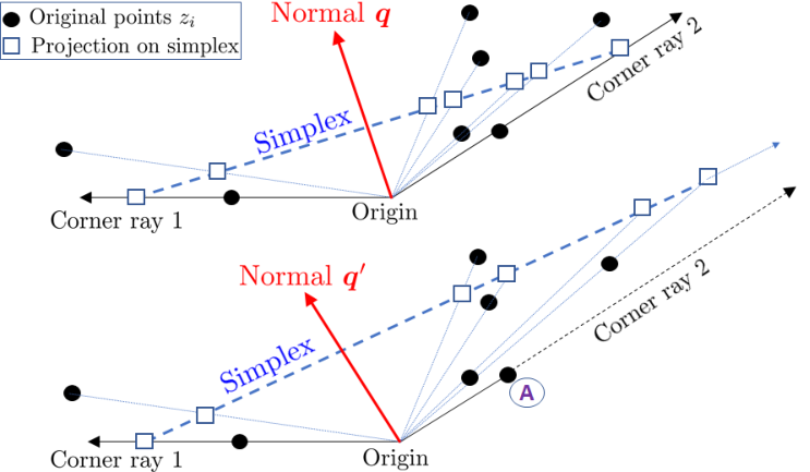
Figure 1: (a) Simplex-based corner-finding methods require points on a simplex, with uniformly small errors. Projecting points to a simplex with normal vector 𝒒\bm{q} works well, but a very similar 𝒒′\bm{q}^{\prime} does not. Some points (such as Ⓐ) get projected to far-off points, amplifying errors in their positions. (b) Instead, we normalize points to the unit sphere, and (c) find corners from the support vectors of a one-class SVM.

Let us illustrate why seemingly obvious methods fail to obtain the corner rays. The simplest idea would be to generate a random plane (the “simplex”), and project points to the intersection of the line joining these points to this random plane as shown in Figure 1(a). Corners of this simplex correspond to the corner rays. However, extending the idea to the sample or empirical cone is difficult, because if the simplex is not good, some points can get projected to arbitrarily far points, which will amplify their error. As Figure 1(a) shows, the set of good simplexes may be quite limited, and finding a good simplex is difficult.

We will illustrate our idea with the “ideal cone.” First, we row-normalize the ideal data matrix to have unit ℓ2\ell_{2} norm (similar to Ng et al. [24], Qin and Rohe [27]). This projects all points inside the cone to the surface of the sphere, with the points on the corner rays being projected to the corners (Figure 1(b)).

Then, we show a rather fascinating result, namely, for all the above models, the corners can be obtained via the support vectors of a one class SVM [31], where all normalized points are in the positive class, and the origin is in the negative class (Figure 1(c)). Observe that a hyperplane through the corners separates all the points from the origin. We also show that if the row-wise error of 𝐑{\bf R} is small, the SVM approach can be used to infer 𝐆{\bf G} from empirical cones. Finally, we show that since the row-wise error of 𝐑{\bf R} is indeed small for different degree-corrected overlapping network models and topic models, we can use our algorithm to infer the parameters consistently. We provide error bounds for parameter estimates at the per-node and per-word level, in contrast to typical bounds for the entire parameter matrix. We conclude with experimental results on simulated and real datasets.

2 Proposed work

Consider a population matrix 𝐏{\bf P} of the form 𝐏=ρ​𝚪​𝚯​𝐁​𝚯T​𝚪{\bf P}=\rho{\bm{\Gamma}}{\bm{\Theta}}{\bf B}{\bm{\Theta}}^{T}{\bm{\Gamma}}, with 𝚪∈ℝ>0n×n{\bm{\Gamma}}\in\mathbb{R}_{>0}^{n\times n} being a positive diagonal matrix, 𝚯∈ℝ≥0n×K{\bm{\Theta}}\in\mathbb{R}_{\geq 0}^{n\times K} a community-membership matrix, and 𝐁∈ℝ≥0K×K{\bf B}\in\mathbb{R}_{\geq 0}^{K\times K} a cross-community connection matrix. We will make the following assumptions which are common in the literature:

Assumption 2.1.

(a) Pure nodes: Each community has at least one “pure” node, which belongs solely to that community. (b) Non-zero rows: No row of 𝚯{\bm{\Theta}} is identically 00. (c) 𝐁{\bf B} is full rank.

The form of the population matrix 𝐏{\bf P}, alongside Assumption 2.1, induces a conic structure on the rows of the eigenvectors of 𝐏{\bf P}.

Lemma 2.1.

Let there be KK communities (rank⁡(𝐏)=K\mathrm{rank}({\bf P})=K), and let ℐ\mathcal{I} be indices of KK pure nodes, one from each community. Let 𝐏=𝐕𝐄𝐕T{\bf P}={\bf V}{\bf E}{\bf V}^{T} be the top-KK eigen-decomposition of 𝐏{\bf P}, where columns of 𝐕∈ℝn×K{\bf V}\in\mathbb{R}^{n\times K} are the KK principal eigenvectors and 𝐄∈ℝK×K{\bf E}\in\mathbb{R}^{K\times K} is a diagonal matrix of the KK principal eigenvalues. Then, 𝐕=𝚪​𝚯​𝚪P−1​𝐕P{\bf V}={\bm{\Gamma}}{\bm{\Theta}}{\bm{\Gamma}}_{P}^{-1}{\bf V}_{P}, where 𝐕P=𝐕(ℐ,:){\bf V}_{P}={\bf V}(\mathcal{I},:) is full rank and 𝚪P=𝚪⁡(ℐ,ℐ){\bm{\Gamma}}_{P}={\bm{\Gamma}}(\mathcal{I},\mathcal{I}).

Since (𝚪​𝚯​𝚪P−1)i​j≥0({\bm{\Gamma}}{\bm{\Theta}}{\bm{\Gamma}}_{P}^{-1})_{ij}\geq 0 for all (i,j)(i,j), the rows of 𝐕{\bf V} fall within a cone with corners 𝐕P{\bf V}_{P}. This suggests the following idealized problem:

Problem 1 (Ideal cone problem).

We are given a matrix 𝐙∈ℝn×m{\bf Z}\in\mathbb{R}^{n\times m} such that 𝐙=𝐌𝐘P{\bf Z}={\bf M}{\bf Y}_{P}, where 𝐌∈ℝ≥0n×K{\bf M}\in\mathbb{R}_{\geq 0}^{n\times K}, no row of 𝐌{\bf M} is 00, and 𝐘P∈ℝK×m{\bf Y}_{P}\in\mathbb{R}^{K\times m} corresponds to KK (unknown) rows of 𝐙{\bf Z}, each scaled to unit ℓ2\ell_{2} norm. Infer 𝐌{\bf M} from 𝐙{\bf Z}.

The rows of 𝐘P{\bf Y}_{P} are unit vectors representing the corner rays of the cone. Each row of 𝐙{\bf Z} is constructed from a non-negative weighted combination of these unit vectors, with the weights being given by the corresponding rows of 𝐌{\bf M}. Rows of 𝐙{\bf Z} that lie on some corner correspond to rows of 𝐌{\bf M} that have zero in all but one component. Observe that 𝐌{\bf M} is invariant to the choice of KK corner rows of 𝐙{\bf Z} used to construct 𝐘P{\bf Y}_{P}.

Now consider solving the ideal cone problem with the eigenvector matrix, i.e., 𝐙=𝐕{\bf Z}={\bf V}. From Lemma 2.1, the corner rows correspond to the pure nodes. Choosing one such row from each corner gives us a set of pure node indices ℐ\mathcal{I}. Hence, 𝐌=𝚪​𝚯​𝚪P−1​𝐍P−1{\bf M}={\bm{\Gamma}}{\bm{\Theta}}{\bm{\Gamma}}_{P}^{-1}{\bf N}_{P}^{-1}, where 𝐍{\bf N} is a diagonal matrix with 𝐍i​i=1/‖𝐞iT​𝐙‖{\bf N}_{ii}=1/\|{\bf e}_{i}^{T}{\bf Z}\| and 𝐍P=𝐍(ℐ,:){\bf N}_{P}={\bf N}(\mathcal{I},:). We also have the identity ρ​𝚪P​𝐁​𝚪P=𝐕P​𝐄𝐕PT\rho{\bm{\Gamma}}_{P}{\bf B}{\bm{\Gamma}}_{P}={\bf V}_{P}{\bf E}{\bf V}_{P}^{T}. Coupled with model-specific identifiability conditions (details are provided in the Appendix), these can be used to infer 𝚯{\bm{\Theta}} and ρ​𝐁\rho{\bf B} (𝚪{\bm{\Gamma}} are typically considered nuisance parameters).

In practice, we only have an observation matrix 𝐀{\bf A} that is stochastically generated from the population matrix 𝐏{\bf P}. Hence, we must actually solve:

Problem 2 (Empirical cone problem).

We are given a matrix 𝐙^∈ℝn×m\hat{{\bf Z}}\in\mathbb{R}^{n\times m} such that maxi∈[n]⁡‖𝐞iT​(𝐘−𝐘^)‖2≤ϵ\max_{i\in[n]}\|{\bf e}_{i}^{T}({\bf Y}-\hat{{\bf Y}})\|_{2}\leq\epsilon, where 𝐘=𝐍𝐙{\bf Y}={\bf N}{\bf Z} is the row-normalized version of 𝐙{\bf Z}, and 𝐘^\hat{{\bf Y}} is constructed similarly from 𝐙^\hat{{\bf Z}}. Again, 𝐙=𝐌𝐘P{\bf Z}={\bf M}{\bf Y}_{P}, where 𝐌≥0{\bf M}\geq 0, no row of 𝐌{\bf M} is 00, and 𝐘P=𝐘(ℐ,:){\bf Y}_{P}={\bf Y}(\mathcal{I},:) corresponds to KK (unknown) rows of 𝐘{\bf Y} with indices ℐ\mathcal{I}. Infer 𝐌{\bf M} from 𝐙^\hat{{\bf Z}}.

We will first present the solution to the ideal cone problem. We will then show that the same algorithm with some post-processing solves the empirical cone problem up to O⁡(ϵ)O(\epsilon) error. Finally, we apply our algorithm to infer parameters for a variety of models, and present error bounds for each.

Notation: We shall refer to the it​hi^{th} row of 𝐙{\bf Z} as 𝐳iT{\bf z}_{i}^{T} expressed using a column vector, i.e., 𝐳i=𝐙T​𝐞i{\bf z}_{i}={\bf Z}^{T}{\bf e}_{i}. The same pattern will be used for rows 𝒎iT\bm{m}_{i}^{T} of 𝐌{\bf M}, and other matrices as well.

2.1 The Ideal Cone Problem

Observe that given the corner indices ℐ\mathcal{I} (i.e., given 𝐘P{\bf Y}_{P}), finding 𝐌{\bf M} such that 𝐙=𝐌𝐘P{\bf Z}={\bf M}{\bf Y}_{P} is a simple regression problem. Thus, the only difficulty is in finding the corner indices.

Our key insight is that under certain conditions, the ideal cone problem can be solved easily by a one-class SVM applied to the rows of 𝐘{\bf Y}. Figure 1 plots the normalized rows 𝐲i{\bf y}_{i} of 𝐘{\bf Y} for an example cone. Observe that a hyperplane through the corners separates all the points from the origin. This suggests that the normalized corners are the support vectors found by a one-class SVM:

maximize ​b s.t. ​𝐰T​𝐲i≥b⁡(for ​i=1,…,n)​ and ​‖𝐰‖2≤1.\text{maximize }\ b\hskip 10.00002pt\text{ s.t. }{\bf w}^{T}{\bf y}_{i}\geq b\;(\text{for }i=1,\ldots,n)\text{ and }\|{\bf w}\|_{2}\leq 1. (1)

We show next that this intuition is correct. Define the following condition.

Condition 1.

The matrix 𝐘P{\bf Y}_{P} satisfies (𝐘P​𝐘PT)−1​𝟏>0({\bf Y}_{P}{\bf Y}_{P}^{T})^{-1}{\bf 1}>0.

Theorem 2.2.

Each support vector selected by the one-class SVM (Eq. 1) is a corner of Z. Also, if Condition 1 holds, there is at least one support vector for every corner.

Thus, under Condition 1, we can get all the corners from the support vectors, and then find 𝐌{\bf M} via regression of 𝐙{\bf Z} on 𝐘P{\bf Y}_{P}. Condition 1 is always satisfied for our problem setting, as shown next.

Theorem 2.3.

Let 𝐏{\bf P} be a population matrix satisfying Assumption 2.1. Let 𝐙=𝐕{\bf Z}={\bf V}, where 𝐕{\bf V} is the rank-KK eigenvector matrix. Let 𝐘=𝐍𝐙{\bf Y}={\bf N}{\bf Z} as defined above. Then, Condition 1 is true.

Thus, the ideal cone problem is easily solved by a one-class SVM. Next, we show that the same method suffices for the empirical cone problem too.

2.2 The Empirical Cone Problem

Now, instead of the normalized eigenvector rows 𝐘{\bf Y}, we are given the empirical matrix 𝐘^\hat{{\bf Y}} with rows 𝐳^iT/‖𝐳^i‖\hat{{\bf z}}_{i}^{T}/\|\hat{{\bf z}}_{i}\|, where maxi⁡‖𝐞iT​(𝐘^−𝐘)‖≤ϵ\max_{i}\|{\bf e}_{i}^{T}(\hat{{\bf Y}}-{\bf Y})\|\leq\epsilon. Once again, we focus on finding the corner indices, using which 𝐌{\bf M} can be inferred by regression. We will show that running a one-class SVM on the rows of 𝐘^\hat{{\bf Y}} yields “near-corners,” after some post-processing. We will need a stronger form of Condition 1:

Condition 2.

The matrix 𝐘P{\bf Y}_{P} satisfies (𝐘P​𝐘PT)−1​𝟏≥η​𝟏{({\bf Y}_{P}{\bf Y}_{P}^{T})^{-1}{\bf 1}}\geq\eta{\bf 1} for some constant η>0\eta>0.

It is easy to show that the solution (𝐰,b)({\bf w},b) of the population SVM under Condition 1 is given by

𝐰\displaystyle{\bf w} =b−1⋅𝐘PT​𝜷\displaystyle=b^{-1}\cdot{\bf Y}_{P}^{T}{\bm{\beta}} b\displaystyle b =(𝟏T(𝐘P𝐘PT)−1𝟏)−1/2\displaystyle=\left({\bf 1}^{T}({\bf Y}_{P}{\bf Y}_{P}^{T})^{-1}{\bf 1}\right)^{-1/2} 𝜷\displaystyle{\bm{\beta}} =(𝐘P​𝐘PT)−1​𝟏𝟏T​(𝐘P​𝐘PT)−1​𝟏.\displaystyle=\dfrac{({\bf Y}_{P}{\bf Y}_{P}^{T})^{-1}{\bf 1}}{{\bf 1}^{T}({\bf Y}_{P}{\bf Y}_{P}^{T})^{-1}{\bf 1}}. (2)

Thus, Condition 1 implies that 𝐰{\bf w} is a convex combination of the corners, while Condition 2 additionally requires a minimum contribution from each corner.

Lemma 2.4 (SVM solution is nearly ideal).

Let (𝐰^,b^)(\hat{{\bf w}},\hat{b}) be the solution for the one-class SVM (Eq. 1) applied to the rows of 𝐘^\hat{{\bf Y}}. Under Condition 2, we have |b^−b|≤ϵ|\hat{b}-b|\leq\epsilon and ‖𝐰^−𝐰‖≤ζ​ϵ\|\hat{{\bf w}}-{\bf w}\|\leq\zeta\epsilon, for ζ=4η​b2​λK​(𝐘P​𝐘PT)≤4​Kη​(λK​(𝐘P​𝐘PT))1.5\zeta=\frac{4}{\eta b^{2}\sqrt{\lambda_{K}({{\bf Y}}_{P}{{\bf Y}}_{P}^{T})}}\leq\frac{4K}{\eta(\lambda_{K}({{\bf Y}}_{P}{{\bf Y}}_{P}^{T}))^{1.5}}.

Unlike the ideal cone scenario, the rows 𝐘^P\hat{{\bf Y}}_{P} corresponding to the corners need not be support vectors for the empirical cone. However, they are not far off.

Lemma 2.5 (Corners are nearly support vectors).

The corners of the population cone are close to the supporting hyperplane: b^​𝟏≤𝐘^P​𝐰^≤b^​𝟏+(ζ+2)​ϵ​𝟏\hat{b}{\bf 1}\leq\hat{{{\bf Y}}}_{P}\hat{\bf w}\leq\hat{b}{\bf 1}+(\zeta+2)\epsilon{\bf 1}.

This suggests that we should consider all points that are up to (ζ+2)​ϵ(\zeta+2)\epsilon away from the supporting hyperplane when searching for corners. The next Lemma shows that each such point is a “near-corner.”

Recall that each row 𝐲^iT\hat{{\bf y}}_{i}^{T} is a noisy version of a population row 𝐲iT=𝒎iT​𝐘P/‖𝒎iT​𝐘P‖{\bf y}_{i}^{T}=\bm{m}_{i}^{T}{\bf Y}_{P}/\|\bm{m}_{i}^{T}{\bf Y}_{P}\|, which can be rewritten as a scaled convex combination of the normalized corners: 𝐲iT=ri​ϕiT​𝐘P{{\bf y}_{i}^{T}=r_{i}{\bm{\phi}}_{i}^{T}{\bf Y}_{P}}, where ϕiT​𝟏=1{\bm{\phi}}_{i}^{T}{\bf 1}=1. Specifically, ri=𝒎iT​𝟏‖𝒎iT​𝐘P‖r_{i}=\frac{\bm{m}_{i}^{T}{\bf 1}}{\|\bm{m}_{i}^{T}{\bf Y}_{P}\|} and ϕi=𝒎i𝒎iT​𝟏{\bm{\phi}}_{i}=\frac{\bm{m}_{i}}{\bm{m}_{i}^{T}{\bf 1}}. For a corner, ri=1r_{i}=1 and ϕi=𝐞j{\bm{\phi}}_{i}={\bf e}_{j} for some jj. We now show that every point ii that is close to the supporting hyperplane is nearly a corner of the ideal cone.

Lemma 2.6 (Points close to support vectors are near-corners).

If 𝐰^T​𝐲^i≤b^+(ζ+2)​ϵ\hat{\bf w}^{T}\hat{{{\bf y}}}_{i}\leq\hat{b}+(\zeta+2)\epsilon for some point i∈[n]i\in[n], then 1≤ri≤1+(ζ+4)​ϵb−ϵ1\leq r_{i}\leq 1+\frac{(\zeta+4)\epsilon}{b-\epsilon} and ϕi​j≥1−2​ζ​ϵb​λK​(𝐘P​𝐘PT)\phi_{ij}\geq 1-\frac{2\zeta\epsilon}{b\lambda_{K}({{\bf Y}}_{P}{{\bf Y}}_{P}^{T})} for some j∈[K]j\in[K].

Consider the set of points Sc={i∣𝐰^T​𝐲^i≤b^+(ζ+2)​ϵ}S_{c}=\{i\mid\hat{\bf w}^{T}\hat{{{\bf y}}}_{i}\leq\hat{b}+(\zeta+2)\epsilon\} that are close to the supporting hyperplane. Lemmas 2.5 and 2.6 show that ScS_{c} contains all corners, and possibly other points that are all near-corners. This suggests that we can cluster the vectors {𝐲^i∣i∈S}\{\hat{{{\bf y}}}_{i}\mid i\in S\} into KK clusters, each corresponding to one corner and possibly extra near-corners close to that corner. Randomly selecting one point from each cluster gives us the set of inferred corners.

Lemma 2.7 (Each corner has its own cluster).

There exist exactly KK clusters in ScS_{c}, as long as ϵ≤cϵ​η​(λK​(𝐘P​𝐘PT))3K1.5​κ⁡(𝐘P​𝐘PT)\epsilon\leq c_{\epsilon}\frac{\eta(\lambda_{K}({{\bf Y}}_{P}{{\bf Y}}_{P}^{T}))^{3}}{K^{1.5}\sqrt{\kappa({{\bf Y}}_{P}{{\bf Y}}_{P}^{T})}}, for some global constant cϵc_{\epsilon}.

Let CC be the indices of the near-corners picked by this clustering step. Since 𝐙=𝐌𝐘P{\bf Z}={\bf M}{\bf Y}_{P}, this suggests 𝐌{\bf M} can be obtained via regression: 𝐌≈𝐙^​𝐘^CT​(𝐘^C​𝐘^CT)−1​𝚷{\bf M}\approx\hat{{\bf Z}}\hat{{{\bf Y}}}_{C}^{T}(\hat{{{\bf Y}}}_{C}\hat{{{\bf Y}}}_{C}^{T})^{-1}{\bf\Pi}, where 𝐘^C:=𝐘^(C,:){\hat{{{\bf Y}}}_{C}:=\hat{{{\bf Y}}}(C,:)} and 𝚷{\bf\Pi} is a permutation matrix that matches the ordering of ideal corners and the empirical near-corners.

Theorem 2.8.

If Condition 2 and the condition on ϵ\epsilon in Lemma 2.7 holds, then for any i∈[n]i\in[n], ‖𝐞iT​(𝐌−𝐙^​𝐘^CT​(𝐘^C​𝐘^CT)−1​𝚷)‖≤cM​κ​(𝐘P​𝐘PT)​‖𝐞iT​𝐙‖​K​ζ(λK​(𝐘P​𝐘PT))2.5​ϵ,{\|{\bf e}_{i}^{T}({\bf M}-\hat{{\bf Z}}\hat{{{\bf Y}}}_{C}^{T}(\hat{{{\bf Y}}}_{C}\hat{{{\bf Y}}}_{C}^{T})^{-1}{\bf\Pi})\|\leq\frac{c_{M}\kappa({{\bf Y}}_{P}{{\bf Y}}_{P}^{T})\|{\bf e}_{i}^{T}{\bf Z}\|{K\zeta}}{(\lambda_{K}({{\bf Y}}_{P}{{\bf Y}}_{P}^{T}))^{2.5}}\epsilon,} where cMc_{M} is a global constant, and κ(.)\kappa(.) is the ratio of the largest and smallest nonzero singular values of a matrix.

Algorithm 1 shows all the steps of our method (SVM-cone). The algorithm requires an estimate of δ:=(ζ+2)​ϵ\delta:=(\zeta+2)\epsilon, and returns the inferred 𝐌{\bf M} and near-corners CC. When the row-wise error bound ϵ\epsilon is unknown, we can start with δ=0\delta=0 and incrementally increase it until KK distinct clusters are found.

Algorithm 1 SVM-cone
0:  𝐙^∈ℝn×m\hat{{\bf Z}}\in\mathbb{R}^{n\times m}, number of corners KK, estimated distance of corners from hyperplane δ\delta
0:  Estimated conic combination matrix 𝐌^\hat{{\bf M}} and near-corner set CC
1:  Normalize rows of 𝐙^\hat{{\bf Z}} by ℓ2\ell_{2} norm to get 𝐘^\hat{{{\bf Y}}} with rows 𝐲^iT\hat{{\bf y}}_{i}^{T}
2:  Run one-class SVM on 𝐲^i\hat{{\bf y}}_{i} to get the normal 𝐰^\hat{\bf w} and distance b^\hat{b} of the supporting hyperplane
3:  Cluster points {𝐲^i∣𝐰^T​𝐲^i≤b^+δ}\{\hat{{\bf y}}_{i}\mid\hat{\bf w}^{T}\hat{{{\bf y}}}_{i}\leq\hat{b}+\delta\} that are close to the hyperplane into KK clusters
4:  Pick one point from each cluster to get near-corner set CC
5:  𝐌^=𝐙^​𝐘^CT​(𝐘^C​𝐘^CT)−1\hat{{\bf M}}=\hat{{\bf Z}}\hat{{{\bf Y}}}_{C}^{T}(\hat{{{\bf Y}}}_{C}\hat{{{\bf Y}}}_{C}^{T})^{-1}

3 Applications

Many network models and topic models have population matrices of the form 𝐏=ρ​𝚪​𝚯​𝐁​𝚯T​𝚪{\bf P}=\rho{\bm{\Gamma}}{\bm{\Theta}}{\bf B}{\bm{\Theta}}^{T}{\bm{\Gamma}}. We have already shown that in such cases, the eigenvector matrix 𝐕{\bf V} forms an ideal cone (Lemma 2.1), and that Condition 1 holds. It is easy to see that the same holds for 𝐕𝐕T{\bf V}{\bf V}^{T} as well. This suggests that SVM-cone can be applied to the matrix 𝐕^​𝐕^T\hat{{\bf V}}\hat{{\bf V}}^{T}, where 𝐕^\hat{{\bf V}} is the empirical top-KK eigenvector matrix. We shall show that this yields per-node error bounds in estimating community memberships and per-word error bounds for word-topic distributions.

3.1 Network models

Define a “DCMMSB-type” model as a model with population matrix 𝐏=ρ​𝚪​𝚯​𝐁​𝚯T​𝚪{\bf P}=\rho{\bm{\Gamma}}{\bm{\Theta}}{\bf B}{\bm{\Theta}}^{T}{\bm{\Gamma}} and an empirical adjacency matrix 𝐀{\bf A} with 𝐀j​i=𝐀i​j∼Bernoulli​(𝐏i​j){\bf A}_{ji}={\bf A}_{ij}\sim\text{Bernoulli}({\bf P}_{ij}) for all i>ji>j. Assume that rows of 𝚯{\bm{\Theta}} have unit ℓp\ell_{p} norm, for p=1p=1 (DCMMSB) or p=2p=2 (OCCAM [36]). Let 𝐯i=𝐕T​𝐞i{\bf v}_{i}={\bf V}^{T}{\bf e}_{i}, 𝐯^i=𝐕^T​𝐞i\hat{\bf v}_{i}=\hat{\bf V}^{T}{\bf e}_{i}, 𝐲i=𝐕𝐯i/‖𝐕𝐯i‖{{\bf y}}_{i}={\bf V}{\bf v}_{i}/\|{\bf V}{\bf v}_{i}\|, and 𝐲^i=𝐕^​𝐯^i/‖𝐕^​𝐯^i‖\hat{{{\bf y}}}_{i}=\hat{\bf V}\hat{\bf v}_{i}/\|\hat{\bf V}\hat{\bf v}_{i}\|. Denote γmax=maxi⁡𝚪i​i\gamma_{\max}=\max_{i}{\bm{\Gamma}}_{ii} and γmin=mini⁡𝚪i​i\gamma_{\min}=\min_{i}{\bm{\Gamma}}_{ii}.

Theorem 3.1 (Small row-wise error in Network Models).

Consider a DCMMSB-type model with 𝛉i∼Dirichlet⁡(𝛂){\bm{\theta}}_{i}\sim\mathrm{Dirichlet}({\bm{\alpha}}), and α0:=𝛂T​𝟏\alpha_{0}:={\bm{\alpha}}^{T}{\bf 1}. If ν:=α0αmin≤min⁡(n27​log⁡n,γmin2γmax2​n​ρ)2​(1+α0)\nu:=\dfrac{\alpha_{0}}{\alpha_{\min}}\leq\dfrac{\min(\sqrt{\frac{n}{27\log n}},{\frac{\gamma_{\min}^{2}}{\gamma_{\max}^{2}}n\rho})}{2(1+\alpha_{0})}, λ∗​(𝐁)ν≥8​(1+α0)​(log⁡n)ξγmin2​n​ρ{\dfrac{\lambda^{*}({\bf B})}{\nu}\geq\dfrac{8(1+\alpha_{0})(\log n)^{\xi}}{\gamma_{\min}^{2}\sqrt{n\rho}}} for some constant ξ>1\xi>1, κ⁡(𝚯T​𝚪2​𝚯)=Θ⁡(1)\kappa({\bm{\Theta}}^{T}{\bm{\Gamma}}^{2}{\bm{\Theta}})=\Theta(1), and α0=O⁡(1)\alpha_{0}=O(1), then

ϵ=maxi⁡‖𝐲i−𝐲^i‖=O~​(γmax​min⁡{K2,(κ⁡(𝐏))2}​K0.5​ν​(1+α0)γmin3​λ∗​(𝐁)​n​ρ)\displaystyle\epsilon=\max_{i}\|{{\bf y}}_{i}-\hat{{{\bf y}}}_{i}\|=\tilde{O}\left(\frac{\gamma_{\max}\min\{K^{2},(\kappa({\bf P}))^{2}\}K^{0.5}\nu(1+\alpha_{0})}{\gamma_{\min}^{3}\lambda^{*}({\bf B})\sqrt{n\rho}}\right)

with probability at least 1−O⁡(K​n−2)1-O(Kn^{-2}). Here λ∗​(𝐁)\lambda^{*}({\bf B}) is the smallest singular value of 𝐁{\bf B}.

Similar results for the non-Dirichlet case follow easily as long as n​ρ=Ω⁡((log⁡n)2​ξ)n\rho=\Omega((\log n)^{2\xi}), λK​(𝐏)=Ω⁡(n​ρ​(log⁡n)ξ)\lambda_{K}({\bf P})=\Omega(\sqrt{n\rho}(\log n)^{\xi}), and maxi∥𝐕(:,i)∥=O(ρ)\max_{i}\|{\bf V}(:,i)\|=O(\sqrt{\rho}) with high probability. This shows that the rows of 𝐕^​𝐕^T\hat{{\bf V}}\hat{{\bf V}}^{T} are close to those of 𝐕𝐕T{\bf V}{\bf V}^{T}, and the latter forms an ideal cone satisfying Condition 1. Hence, the conic combination for each node can be recovered by Algorithm 1 applied to 𝐕^​𝐕^T\hat{{\bf V}}\hat{{\bf V}}^{T}. In fact, we can run the algorithm on 𝐕^\hat{{\bf V}} itself; the output depends only on the SVM dual variables 𝜷{\bm{\beta}} (Eq. 2), which are the same whether the input is 𝐕^\hat{{\bf V}} or 𝐕^​𝐕^T\hat{{\bf V}}\hat{{\bf V}}^{T}. The output is the same conic combination matrix 𝐌^\hat{{\bf M}} and the same set CC of nearly-pure nodes.

For identifiability of 𝚯{\bm{\Theta}}, we need another condition. We will assume that ∑𝚪i​i=n\sum{\bm{\Gamma}}_{ii}=n and all diagonal entries of 𝐁{\bf B} are equal (details are provided in the Appendix). The next theorem shows that SVM-cone can be used to consistently infer the parameters of DCMMSB as well as OCCAM [36].

Theorem 3.2 (Consistent inference of community memberships for each node).

Consider DCMMSB-type models where the conditions of Theorem 3.1 are satisfied and κ⁡(𝚯T​𝚪2​𝚯)=Θ⁡(1){\kappa({\bm{\Theta}}^{T}{\bm{\Gamma}}^{2}{\bm{\Theta}})=\Theta(1)}. Let 𝐃^\hat{{\bf D}} be a diagonal matrix with entries 𝐃^i​i=𝐞iT​𝐘^C​𝐕^​𝐄^​𝐕^T​𝐘^CT​𝐞i\hat{{\bf D}}_{ii}=\sqrt{{\bf e}_{i}^{T}\hat{{{\bf Y}}}_{C}\hat{\bf V}\hat{{\bf E}}\hat{\bf V}^{T}\hat{{{\bf Y}}}_{C}^{T}{\bf e}_{i}}. Let 𝚯^=𝐅^−1​𝐌^​𝐃^\hat{{\bm{\Theta}}}=\hat{{\bf F}}^{-1}\hat{{\bf M}}\hat{{\bf D}}, where 𝐅^\hat{{\bf F}} is a diagonal matrix with entries 𝐅^i​i=‖𝐞iT​𝐌^​𝐃^‖1\hat{{\bf F}}_{ii}=\|{\bf e}_{i}^{T}\hat{{\bf M}}\hat{{\bf D}}\|_{1} (for DCMMSB) and 𝐅^i​i=‖𝐞iT​𝐌^​𝐃^‖2{\hat{{\bf F}}_{ii}=\|{\bf e}_{i}^{T}\hat{{\bf M}}\hat{{\bf D}}\|_{2}} (for OCCAM [36]). Then there exists a permutation matrix 𝚷{\bf\Pi} such that

‖𝐞iT​(𝚯−𝚯^​𝚷)‖\displaystyle{\|{\bf e}_{i}^{T}({\bm{\Theta}}-\hat{{\bm{\Theta}}}{\bf\Pi})\|} =O~​(γmax​K2.5​min⁡{K2,(κ⁡(𝐏))2}​n3/2γmin​η​λ∗​(𝐁)​λK2​(𝚯T​𝚪2​𝚯)​ρ)\displaystyle=\tilde{O}\left(\frac{\gamma_{\max}K^{2.5}\min\{K^{2},(\kappa({\bf P}))^{2}\}n^{3/2}}{\gamma_{\min}\eta\lambda^{*}({\bf B})\lambda_{K}^{2}({\bm{\Theta}}^{T}{\bm{\Gamma}}^{2}{\bm{\Theta}})\sqrt{\rho}}\right)

with probability at least 1−O⁡(K​n−2)1-O(Kn^{-2}).

Remark 3.1.

The error bound is small when the clusters are well separated (large λ∗​(𝐁)\lambda^{*}({\bf B})), the network is dense (large ρ\rho), there are few blocks (small KK), and the membership vectors 𝚯{\bm{\Theta}} are drawn from a balanced Dirichlet distribution (small ν\nu, and hence small κ⁡(P)\kappa(P)), which leads to balanced block sizes.

Remark 3.2.

For DCMMSB-type models, η≥γmin2​mini⁡(𝐞iT​𝚯T​𝟏)λ1​(𝚯T​𝚪2​𝚯)\eta\geq\frac{\gamma_{\min}^{2}\min_{i}({\bf e}_{i}^{T}{\bm{\Theta}}^{T}{\bf 1})}{{\lambda_{1}({\bm{\Theta}}^{T}{\bm{\Gamma}}^{2}{\bm{\Theta}})}}. Also, under the conditions of Theorem 3.1, η≥γmin23​ν​γmax2\eta\geq\frac{\gamma_{\min}^{2}}{3\nu\gamma_{\max}^{2}} with high probability. Proofs are in the Appendix.

Observe that these are per-node error bounds, as against a simpler bound on ‖𝚯−𝚯^‖\|{\bm{\Theta}}-\hat{{\bm{\Theta}}}\|. Clearly, the same results extend to the special case of the Mixed Membership Stochastic Blockmodel [1] and the Stochastic Blockmodel [13] as well (the assumption of equal diagonal entries of 𝐁{\bf B} is no longer needed, since 𝚪i​i=1{\bm{\Gamma}}_{ii}=1 is enough for parameter identifiability [22]).

3.2 Topic Models

Let 𝐓∈ℝ≥0V×K{\bf T}\in\mathbb{R}_{\geq 0}^{V\times K} be a matrix of the word to topic probabilities with unit column sum, and let 𝐇∈ℝ≥0K×D{\bf H}\in\mathbb{R}_{\geq 0}^{K\times D} be the topic to document matrix. Then 𝒜:=𝒯ℋ\mathbfcal{A}:={\bf T}{\bf H} is the probability matrix for words appearing in documents. The actual counts of words in documents are assumed to be generated iid as 𝐀i​j∼Binomial(N,𝒜⟩|){\bf A}_{ij}\sim\text{Binomial}(N,\mathbfcal{A}_{ij}) for i∈[V],j∈[D]i\in[V],j\in[D].

The word co-occurrence probability matrix is given by 𝒜𝒜𝒯/𝒟=𝒯⁡(ℋℋ𝒯/𝒟)​𝒯𝒯\mathbfcal{A}\mathbfcal{A}^{T}/D={\bf T}({\bf H}{\bf H}^{T}/D){\bf T}^{T}. Setting 𝚪i​i=∥𝐓(i,:)∥1{\bm{\Gamma}}_{ii}=\|{\bf T}(i,:)\|_{1}, 𝚯=𝚪−1​𝐓{\bm{\Theta}}={\bm{\Gamma}}^{-1}{\bf T}, and 𝐁=𝐇𝐇T/D{\bf B}={\bf H}{\bf H}^{T}/D, we find that 𝒜𝒜𝒯/𝒟=𝚪​𝚯​ℬ​𝚯𝒯​𝚪\mathbfcal{A}\mathbfcal{A}^{T}/D={\bm{\Gamma}}{\bm{\Theta}}{\bf B}{\bm{\Theta}}^{T}{\bm{\Gamma}} with 𝚯​𝟏=𝟏{\bm{\Theta}}{\bf 1}={\bf 1}. This clearly matches the form of 𝐏{\bf P} in the DCMMSB model. Hence, its eigenvector matrix has the desired conic structure with weight matrix 𝐌=𝐓​𝚪P−1​𝐍P−1{\bf M}={\bf T}{\bm{\Gamma}}_{P}^{-1}{\bf N}_{P}^{-1}, with the “pure nodes” being anchor words that only occur in a single topic. We now show that the row-wise error between the empirical and population eigenvector matrices decays with increasing number of documents DD and number of words in a document NN.

Assumption 3.1.

Let gi​k=𝐞iT𝒜𝒜𝒯⌉∥g_{ik}={\bf e}_{i}^{T}\mathbfcal{A}\mathbfcal{A}^{T}e_{k}. We assume that when it is not zero, it goes to infinity, in particular, gi​k≥N​log⁡max⁡(V,D)g_{ik}\geq N\log\max(V,D), which gives D/N→∞D/N\rightarrow\infty. We also assume that λi​(𝐇𝐇T)=Θ⁡(D)\lambda_{i}({\bf H}{\bf H}^{T})=\Theta(D), for i∈[K]i\in[K], and κ⁡(𝐓𝐓T)=Θ⁡(1)\kappa({\bf T}{\bf T}^{T})=\Theta(1).

These assumptions are similar to ones made in other theoretical literature on topic models [18].

We will construct a matrix 𝐀1​𝐀2T{\bf A}_{1}{\bf A}_{2}^{T}, where 𝐀1{\bf A}_{1} and 𝐀2{\bf A}_{2} are obtained by dividing the words in each document uniformly randomly in two equal parts. This ensures that E⁡[𝐀1​𝐀2T]=𝒜𝒜𝒯\mathrm{E}[{\bf A}_{1}{\bf A}_{2}^{T}]=\mathbfcal{A}\mathbfcal{A}^{T}, which in turn helps establishing concentration of empirical singular vectors as shown in the following lemma. For simplicity denote N1=N/2N_{1}=N/2.

Lemma 3.3 (Small row-wise error in Topic Models).

Let 𝐕^\hat{{\bf V}} denote the matrix of the top-KK singular vectors of 𝐔=𝐀1​𝐀2T/N12{\bf U}={\bf A}_{1}{\bf A}_{2}^{T}/N_{1}^{2}, and let the population counterpart of this be 𝐕{\bf V}. Let 𝐯i=𝐕T​𝐞i{\bf v}_{i}={\bf V}^{T}{\bf e}_{i}, 𝐯^i=𝐕^T​𝐞i\hat{\bf v}_{i}=\hat{\bf V}^{T}{\bf e}_{i}, 𝐲i=𝐕𝐯i/‖𝐕𝐯i‖{{\bf y}}_{i}={\bf V}{\bf v}_{i}/\|{\bf V}{\bf v}_{i}\|, and 𝐲^i=𝐕^​𝐯^i/‖𝐕^​𝐯^i‖\hat{{{\bf y}}}_{i}=\hat{\bf V}\hat{\bf v}_{i}/\|\hat{\bf V}\hat{\bf v}_{i}\|. Under Assumption 3.1, we have:

ϵ=maxi⁡‖𝐲i−𝐲^i‖=1minj⁡‖𝐞iT​𝐓‖1​λK​(𝐓T​𝐓)​OP​(K​log⁡max​(V,D)D​N)\displaystyle\epsilon=\max_{i}\|{{\bf y}}_{i}-\hat{{{\bf y}}}_{i}\|=\frac{1}{\min_{j}\|{\bf e}_{i}^{T}{\bf T}\|_{1}\sqrt{\lambda_{K}({\bf T}^{T}{\bf T})}}O_{P}\left(\sqrt{\frac{K\log\max(V,D)}{DN}}\right)

with probability at least 1−O⁡(1/D2)1-O(1/D^{2}).

Thus, Algorithm 1 run on 𝐕^​𝐕^T\hat{{\bf V}}\hat{{\bf V}}^{T} (or equivalently, just 𝐕^\hat{{\bf V}}) can be used to find the conic combination weights 𝐌^≈𝐌\hat{{\bf M}}\approx{\bf M}. Since 𝐌{\bf M} being the product of 𝐓{\bf T} with a diagonal matrix where 𝐓{\bf T} has unit column sum, we can extract 𝐓^=𝐌^​𝐃^−1\hat{{\bf T}}=\hat{{\bf M}}\hat{{\bf D}}^{-1}, where 𝐃^\hat{{\bf D}} is a diagonal matrix with 𝐃^i​i=∥𝐌^(:,i)∥1\hat{{\bf D}}_{ii}=\|\hat{{\bf M}}(:,i)\|_{1}.

Theorem 3.4 (Consistent inference of word-topic probabilities for each word).

Under Assumption 3.1, there exists a permutation matrix 𝚷{\bf\Pi} such that

‖𝐞iT​(𝐓^−𝐓​𝚷T)‖‖𝐞iT​𝐓‖=OP​(K4​maxj​‖𝐞jT​𝐓‖1η​(minj⁡‖𝐞jT​𝐓‖1)2​log⁡max⁡(V,D)D​N)\displaystyle\frac{\|{\bf e}_{i}^{T}(\hat{\bf T}-{\bf T}{\bf\Pi}^{T})\|}{\|{\bf e}_{i}^{T}{\bf T}\|}=O_{P}\left(\frac{K^{4}\max_{j}\|{\bf e}_{j}^{T}{\bf T}\|_{1}}{\eta(\min_{j}\|{\bf e}_{j}^{T}{\bf T}\|_{1})^{2}}\sqrt{\frac{\log\max(V,D)}{DN}}\right)

with probability at least 1−O⁡(1/D2)1-O(1/D^{2}).

Remark 3.3.

For topic models, η≥mini⁡‖𝐞iT​𝐓‖1/λ1​(𝐓T​𝐓)≥mini⁡‖𝐞iT​𝐓‖1/K\eta\geq{\min_{i}\|{\bf e}_{i}^{T}{\bf T}\|_{1}}/{{\lambda_{1}({\bf T}^{T}{\bf T})}}\geq{\min_{i}\|{\bf e}_{i}^{T}{\bf T}\|_{1}}/{{K}}. Proofs are in the Appendix.

4 Experiments

We ran experiments on simulated and real-world datasets to verify the accuracy and scalability of SVM-cone. We compared SVM-cone against several competing baselines. For network models, GeoNMF detects the corners of a simplex formed by the MMSB model by constructing the graph Laplacian and picking nodes that have large norms in the Laplacian [21]. It assumes balanced communities (i.e., the rows of 𝚯{\bm{\Theta}} are drawn from a Dirichlet with identical community weights). SVI uses stochastic variational inference for MMSB [12]. BSNMF [26] presents a Bayesian approach to Symmetric Nonnegative Matrix Factorization; it can be applied to do inference for MMSB models with 𝐁=c​𝐈{\bf B}=c{\bf I} where c∈[0,1]c\in[0,1]. OCCAM works on a variant of MMSB where each row of 𝚯{\bm{\Theta}} has unit ℓ2\ell_{2} norm, and the model allows for degree heterogeneity [36]. SAAC [17] uses alternating optimization on a version of the stochastic blockmodel where each node can be a member of multiple communities, but the membership weight is binary. For topic models, RecoverL2 [5] uses a combinatorial algorithm to pick anchor words from the word co-occurrence matrix and then recovers the word-topic vectors by optimizing a quadratic loss function. TSVD [7] uses a thresholded SVD based procedure to recover the topics. GDM [35] is a geometric algorithm that involves a weighted clustering procedure augmented with geometric corrections. We could not obtain the code for [16, 18].

4.1 Networks with overlapping communities

In this section, we present experiments on simulated and large real networks.

4.1.1 Simulations

We test the recovery of population parameters (𝚯,𝐁)({\bm{\Theta}},{\bf B}) given adjacency matrices 𝐀{\bf A} generated from the corresponding population matrices 𝐏{\bf P} (𝚪{\bm{\Gamma}} are nuisance parameters). We generate networks with n=5000n=5000 nodes and K=3K=3 communities. The rows of 𝚯{\bm{\Theta}} are drawn from Dirichlet(𝜶)(\bm{\alpha}) for DCMMSB and OCCAM; for DCMMSB, 𝜶=(1/3,1/3,1/3){\bm{\alpha}}=(1/3,1/3,1/3); for OCCAM, 𝜶=(1/6,1/6,1/6){\bm{\alpha}}=(1/6,1/6,1/6) and the rows are normalized to have unit ℓ2\ell_{2} norm. We set 𝐁i​i=1{\bf B}_{ii}=1 and 𝐁i​j=0.1{\bf B}_{ij}=0.1 for all i≠ji\neq j. The default degree parameters for DCMMSB are as follows: for all nodes ii that are predominantly in the jj-th community (θi​j>0.5\theta_{ij}>0.5), we set 𝚪i​i{\bm{\Gamma}}_{ii} to 0.30.3, 0.50.5, and 0.70.7 for the 3 respective communities; all other nodes have 𝚪i​i=1{\bm{\Gamma}}_{ii}=1. For OCCAM, we draw degree parameters from a Beta⁡(1,3)\mathrm{Beta}(1,3) distribution.

Refer to caption
(a) Varying degree heterogeneity for DCMMSB
Refer to caption
(b) Varying sparsity for DCMMSB
Refer to caption
(c) Varying sparsity for OCCAM model
Refer to caption
(d) Varying sparsity for OSBM
Figure 2: Relative error in estimation of community memberships: Plots (a) and (b) compare SVM-cone against the closest baseline (GeoNMF) on the degree-corrected MMSB model. We then compare against (c) OCCAM and (d) SAAC on networks drawn from their generative models.

Varying degree parameters 𝚪{\bm{\Gamma}}: We set the degree parameters for predominant nodes in the 3 communities as 0.5+ϵΓ0.5+\epsilon_{\Gamma}, 0.50.5, and 0.5+ϵΓ0.5+\epsilon_{\Gamma} respectively. Figure 2(a) shows SVM-cone outperforms GeoNMF consistently for all choices of ϵΓ\epsilon_{\Gamma}.

Varying network sparsity ρ\rho: Figure 2(b) shows the relative error in estimating 𝚯{\bm{\Theta}} as a function of the network sparsity ρ\rho. Increasing ρ\rho increases the average degree of nodes in the network without affecting the skew induced by their degree parameters 𝚪{\bm{\Gamma}}. As expected, all methods tend to improve with increasing degree. Our method dominates GeoNMF over the entire range of average degrees. Figures 2(c) and 2(d) show results for networks generated under the models used by OCCAM and SAAC respectively. SVM-cone is comparable or better than these methods even on their generative models. The smaller error bars on SVM-cone show that it is more stable than SAAC.

4.1.2 Real-world experiments

Table 1: Network statistics
(a) DBLP coauthorship networks.
Dataset DBLP1 DBLP2 DBLP3 DBLP4 DBLP5
#\# nodes nn 30,566 16,817 13,315 25,481 42,351
#\# communities KK 6 3 3 3 4
Average Degree 8.9 7.6 8.5 5.2 6.8
Overlap %\% 18.2 14.9 21.1 14.4 18.5
(b) DBLP bipartite author-paper networks.
Dataset DBLP1 DBLP2 DBLP3 DBLP4 DBLP5
#\# nodes nn 103,660 50,699 42,288 53,369 81,245
#\# communities KK 12 6 6 6 8
Average Degree 3.4 3.4 3.6 2.6 3.0
Overlap %\% 6.3 5.6 5.7 6.9 9.7

We tested SVM-cone on large network datasets and word-document datasets. For networks, we used the 55 DBLP coauthorship networks11 1 http://www.cs.utexas.edu/˜xmao/coauthorship (used in [21], where each ground truth community corresponds to a group of conferences on the same topic. We also use bipartite author-paper variants for these 55 networks. See Table 1(b) for network statistics. Following [21], we evaluate results by the rank correlation between the predicted vector for community ii against the true vector, averaged over all communities: RCa​v​g(𝚯^,𝚯)=1Kmaxσ∑i=1KRC(𝚯^(:,i),𝚯(:,σ(i))){RC_{avg}(\hat{{\bm{\Theta}}},{\bm{\Theta}})=\frac{1}{K}\max_{\sigma}\sum_{i=1}^{K}RC(\hat{{\bm{\Theta}}}(:,i),{\bm{\Theta}}(:,\sigma(i)))}, where σ\sigma is a permutation over the KK communities. We have −1≤R​Ca​v​g​(𝚯^,𝚯)≤1-1\leq RC_{avg}(\hat{{\bm{\Theta}}},{\bm{\Theta}})\leq 1, with higher numbers implying a better match between 𝚯^\hat{{\bm{\Theta}}} and 𝚯{\bm{\Theta}}. We do not use metrics like NMI [32] or ExNVI [36] that require binary overlapping membership vectors to avoid thresholding issues on real-valued membership vectors.

Refer to caption
(a) DBLP coauthorship
Refer to caption
(b) DBLP coauthorship wall-clock time
Refer to caption
(c) DBLP bipartite
Refer to caption
(d) DBLP bipartite wall-clock time
Figure 3: Accuracy of estimated community memberships for (a) the DBLP coauthorship network and (c) the biparite author-paper DBLP network. (b) and (d) The wall-clock time of the competing methods respectively.

We find that SVM-cone outperforms competing baselines on 22 of the 55 DBLP coauthorship datasets, and is similar on the remaining three (Figure 3(a)). The closest competitor is GeoNMF [21], which assumes that all nodes have the same degree parameter, and the community sizes are balanced. Both assumptions are reasonable for the dataset, since the number of coauthors (the degree) does not vary significantly among authors, and the communities are formed from conferences where no one conference dominates the others. The differences between SVM-cone and the competition is starker on the bipartite dataset (Figure 3(c)). There is severe degree heterogeneity: an author can be connected to many papers, while each paper only has a few authors at best. Our method is able to accommodate such differences between the nodes, and hence yields much better accuracy than others.

Finally, Figure 3(b) and 3(d) shows the wall-clock time for running the various methods on DBLP coauthorship networks and DBLP bipartite author-paper networks respectively. Our method is among the fastest. This is expected; the only computationally intensive step is the one-class SVM and top-KK eigen-decomposition (or SVD), for which off-the-shelf efficient and scalable implementations already exist [10].

4.2 Topic Models

We generate semi-synthetic data following [5] and [7] using NIPS11 1 https://archive.ics.uci.edu/ml/datasets/Bag+of+Words, New York Times11 1 https://archive.ics.uci.edu/ml/datasets/Bag+of+Words (NYT), PubMed11 1 https://archive.ics.uci.edu/ml/datasets/Bag+of+Words, and 20NewsGroup22 2 http://qwone.com/~jason/20Newsgroups/ (20NG). Dataset statistics are included in the Appendix. We use Matlab R2018a built-in Gibbs Sampling function for learning topic models to learn the word by topic matrix, which should retain the characteristics of real data distributions. Then we draw the topic-document matrix from Dirichlet with symmetric hyper-parameter 0.01. We set K=40K=40 for the first 3 datasets and K=20K=20 for 20NG. The word counts matrix is sampled with N=1000,300,100,200N=1000,300,100,200 respectively, which matches the mean document length of the real datasets. We evaluate the performance of different algorithms using ℓ1\ell_{1} reconstruction error 1K​∑i,j|𝐓⁡(i,j)−𝐓^​(i,π⁡(j))|\frac{1}{K}\sum_{i,j}|{\bf T}\left(i,j\right)-\hat{{\bf T}}\left(i,\pi(j)\right)|, where π(.)\pi(.) is a permutation function that matches the topics. Table 2 shows the ℓ1\ell_{1} reconstruction error and wall-clock running time of different algorithms with datasets generated from different number of documents. Each setting is repeated 5 times, and we report the mean and standard deviation of the results. SVM-cone is much faster than the other methods. Its accuracy is comparable to RecoverL2, and significantly better than TSVD and GDM. The Appendix also shows the top-10 words of 5 topics learned from SVM-cone for each dataset.

Table 2: ℓ1\ell_{1} reconstruction error and wall-clock time on semi-synthetic datasets
Corpus Documents RecoverL2 TSVD GDM SVM-cone
NIPS 20000 ℓ1\ell_{1} Error 0.059 (±\pm 0.000) 0.237 (±\pm 0.017) 0.081 (±\pm 0.057) 0.071 (±\pm 0.004)
Time/ss 100.11 (±\pm 8.81) 18.54 (±\pm 2.04) 119.66 (±\pm 4.41) 5.33 (±\pm 0.39)
40000 ℓ1\ell_{1} Error 0.043 (±\pm 0.000) 0.250 (±\pm 0.045) 0.061 (±\pm 0.038) 0.051 (±\pm 0.002)
Time/ss 143.34 (±\pm 0.53) 21.97 (±\pm 1.49) 220.92 (±\pm 3.10) 9.07 (±\pm 0.00)
60000 ℓ1\ell_{1} Error 0.036 (±\pm 0.000) 0.269 (±\pm 0.064) 0.059 (±\pm 0.038) 0.041 (±\pm 0.002)
Time/ss 247.34 (±\pm 20.84) 35.77 (±\pm 3.28) 406.87 (±\pm 36.57) 17.63 (±\pm 5.29)
NYT 20000 ℓ1\ell_{1} Error 0.125 (±\pm 0.000) 0.207 (±\pm 0.025) 0.223(±\pm 0.008) 0.131 (±\pm 0.003)
Time/ss 78.15 (±\pm 7.14) 25.11 (±\pm 6.39) 193.43 (±\pm 12.02) 4.51 (±\pm 0.70)
40000 ℓ1\ell_{1} Error 0.103 (±\pm 0.000) 0.197 (±\pm 0.045) 0.216 (±\pm 0.010) 0.106 (±\pm 0.001)
Time/ss 140.84 (±\pm 15.50) 50.18 (±\pm 13.14) 394.16 (±\pm 30.42) 8.04 (±\pm 1.15)
60000 ℓ1\ell_{1} Error 0.095 (±\pm 0.000) 0.166 (±\pm 0.028) 0.210 (±\pm 0.010) 0.096 (±\pm 0.002)
Time/ss 184.69 (±\pm 20.65) 42.96 (±\pm 7.95) 595.54 (±\pm 91.57) 11.82 (±\pm 1.91)
PubMed 20000 ℓ1\ell_{1} Error 0.163 (±\pm 0.000) 0.239 (±\pm 0.032) 0.277 (±\pm 0.051) 0.181 (±\pm 0.002)
Time/ss 54.32 (±\pm 5.94) 15.75 (±\pm 2.34) 205.95 (±\pm 11.27) 2.06 (±\pm 0.46)
40000 ℓ1\ell_{1} Error 0.122 (±\pm 0.000) 0.255 (±\pm 0.018) 0.251 (±\pm 0.041) 0.138 (±\pm 0.001)
Time/ss 78.99 (±\pm 9.99) 26.44 (±\pm 4.49) 459.17 (±\pm 30.71) 3.73 (±\pm 0.37)
60000 ℓ1\ell_{1} Error 0.098 (±\pm 0.000) 0.275 (±\pm 0.041) 0.269 (±\pm 0.052) 0.114 (±\pm 0.001)
Time/ss 98.19 (±\pm 15.06) 24.57 (±\pm 4.59) 649.97 (±\pm 26.48) 5.44 (±\pm 0.38)
20NG 20000 ℓ1\ell_{1} Error 0.100 (±\pm 0.000) 0.111 (±\pm 0.051) 0.137 (±\pm 0.071) 0.090 (±\pm 0.003)
Time/ss 40.74 (±\pm 0.64) 7.51 (±\pm 0.42) 102.86 (±\pm 4.05) 1.85 (±\pm 0.26)
40000 ℓ1\ell_{1} Error 0.074 (±\pm 0.000) 0.081 (±\pm 0.043) 0.131 (±\pm 0.072) 0.064 (±\pm 0.001)
Time/ss 94.42 (±\pm 9.92) 16.04 (±\pm 2.28) 273.51 (±\pm 16.45) 4.33 (±\pm 0.71)
60000 ℓ1\ell_{1} Error 0.058 (±\pm 0.000) 0.133 (±\pm 0.045) 0.096 (±\pm 0.063) 0.052 (±\pm 0.002)
Time/ss 142.34 (±\pm 20.31) 23.36 (±\pm 5.85) 388.47 (±\pm 43.22) 5.89 (±\pm 0.67)

5 Conclusions

We showed that many distinct models for overlapping clustering can be placed under one general framework, where the data matrix is a noisy version of an ideal matrix and each row is a non-negative weighted sum of “exemplars.” In other words, the connection probabilities of one node to others in a network is a non-negative combination of the connection probabilities of KK “pure” nodes to others in the network. Each pure node is an examplar of a single community, and we require one pure node from each of the KK communities. This geometrically corresponds to a cone, with the pure nodes being its corners. This subsumes Mixed-Membership Stochastic Blockmodels and their degree-corrected variants, as well as commonly used topic models. We showed that a one-class SVM applied to the normalized rows of the data matrix can find both the corners and the weight matrix. We proved the consistency of our SVM-cone algorithm, and used it to develop consistent parameter inference methods for several widely used network and topic models. Experiments on simulated and large real-world datasets show both the accuracy and the scalability of SVM-cone.

Acknowledgments

X.M. and P.S. were partially supported by NSF grant DMS 1713082. D.C. was partially supported by a Facebook Faculty Research Award.

References

  • [1] Edoardo M Airoldi, David M Blei, Stephen E Fienberg, and Eric P Xing. Mixed membership stochastic blockmodels. JMLR, 9:1981–2014, 2008.
  • [2] Animashree Anandkumar, Rong Ge, Daniel Hsu, and Sham M. Kakade. A tensor approach to learning mixed membership community models. JMLR, 15(1):2239–2312, 2014a.
  • [3] Animashree Anandkumar, Rong Ge, Daniel Hsu, Sham M Kakade, and Matus Telgarsky. Tensor decompositions for learning latent variable models. The Journal of Machine Learning Research, 15(1):2773–2832, 2014b.
  • [4] Sanjeev Arora, Rong Ge, Ravindran Kannan, and Ankur Moitra. Computing a nonnegative matrix factorization–provably. In STOC, pages 145–162. ACM, 2012.
  • [5] Sanjeev Arora, Rong Ge, Yonatan Halpern, David Mimno, Ankur Moitra, David Sontag, Yichen Wu, and Michael Zhu. A practical algorithm for topic modeling with provable guarantees. In International Conference on Machine Learning, pages 280–288, 2013.
  • [6] Pranjal Awasthi, Bahman Kalantari, and Yikai Zhang. Robust vertex enumeration for convex hulls in high dimensions. In Amos Storkey and Fernando Perez-Cruz, editors, International Conference on Artificial Intelligence and Statistics, volume 84, pages 1387–1396. PMLR, 09–11 Apr 2018.
  • [7] Trapit Bansal, Chiranjib Bhattacharyya, and Ravindran Kannan. A provable svd-based algorithm for learning topics in dominant admixture corpus. In Advances in Neural Information Processing Systems, pages 1997–2005, 2014.
  • [8] Xin Bing, Florentina Bunea, and Marten Wegkamp. A fast algorithm with minimax optimal guarantees for topic models with an unknown number of topics. arXiv preprint arXiv:1805.06837, 2018.
  • [9] David M Blei, Andrew Y Ng, and Michael I Jordan. Latent dirichlet allocation. Journal of machine Learning research, 3(Jan):993–1022, 2003.
  • [10] Chih-Chung Chang and Chih-Jen Lin. Libsvm: a library for support vector machines. ACM transactions on intelligent systems and technology (TIST), 2(3):27, 2011.
  • [11] Weicong Ding, Mohammad Hossein Rohban, Prakash Ishwar, and Venkatesh Saligrama. Topic discovery through data dependent and random projections. In International Conference on Machine Learning, pages 1202–1210, 2013.
  • [12] Prem K Gopalan and David M Blei. Efficient discovery of overlapping communities in massive networks. PNAS, 110(36):14534–14539, 2013.
  • [13] Paul W Holland, Kathryn Blackmond Laskey, and Samuel Leinhardt. Stochastic blockmodels: First steps. Social networks, 5(2):109–137, June 1983. ISSN 0378-8733.
  • [14] Samuel B Hopkins and David Steurer. Bayesian estimation from few samples: community detection and related problems. In FOCS, pages 379–390. IEEE, 2017.
  • [15] Kejun Huang, Xiao Fu, and Nikolaos D Sidiropoulos. Anchor-free correlated topic modeling: Identifiability and algorithm. In Advances in Neural Information Processing Systems, pages 1786–1794, 2016.
  • [16] Jiashun Jin, Zheng Tracy Ke, and Shengming Luo. Estimating network memberships by simplex vertex hunting. arXiv preprint arXiv:1708.07852, 2017.
  • [17] Emilie Kaufmann, Thomas Bonald, and Marc Lelarge. A spectral algorithm with additive clustering for the recovery of overlapping communities in networks. In International Conference on Algorithmic Learning Theory, pages 355–370. Springer, 2016.
  • [18] Zheng Tracy Ke and Minzhe Wang. A new svd approach to optimal topic estimation. arXiv preprint arXiv:1704.07016, 2017.
  • [19] Pierre Latouche, Etienne Birmelé, Christophe Ambroise, et al. Overlapping stochastic block models with application to the french political blogosphere. The Annals of Applied Statistics, 5(1):309–336, 2011.
  • [20] Jing Lei, Alessandro Rinaldo, et al. Consistency of spectral clustering in stochastic block models. The Annals of Statistics, 43(1):215–237, 2015.
  • [21] Xueyu Mao, Purnamrita Sarkar, and Deepayan Chakrabarti. On mixed memberships and symmetric nonnegative matrix factorizations. In ICML, pages 2324–2333, 2017a.
  • [22] Xueyu Mao, Purnamrita Sarkar, and Deepayan Chakrabarti. Estimating mixed memberships with sharp eigenvector deviations. arXiv preprint arXiv:1709.00407, 2017b.
  • [23] Henryk Minc. Nonnegative matrices. 1988.
  • [24] Andrew Y Ng, Michael I Jordan, and Yair Weiss. On spectral clustering: Analysis and an algorithm. In Advances in neural information processing systems, pages 849–856, 2002.
  • [25] Maxim Panov, Konstantin Slavnov, and Roman Ushakov. Consistent estimation of mixed memberships with successive projections. In International Workshop on Complex Networks and their Applications, pages 53–64. Springer, 2017.
  • [26] Ioannis Psorakis, Stephen Roberts, Mark Ebden, and Ben Sheldon. Overlapping community detection using bayesian non-negative matrix factorization. Physical Review E, 83(6):066114, 2011.
  • [27] Tai Qin and Karl Rohe. Regularized spectral clustering under the degree-corrected stochastic blockmodel. In Advances in Neural Information Processing Systems, pages 3120–3128, 2013.
  • [28] Avik Ray, Javad Ghaderi, Sujay Sanghavi, and Sanjay Shakkottai. Overlap graph clustering via successive removal. In 52nd Annual Allerton Conference, pages 278–285. IEEE, 2014.
  • [29] Karl Rohe, Sourav Chatterjee, and Bin Yu. Spectral clustering and the high-dimensional stochastic blockmodel. The Annals of Statistics, pages 1878–1915, 2011.
  • [30] Patrick Rubin-Delanchy, Carey E Priebe, Minh Tang, and Joshua Cape. A statistical interpretation of spectral embedding: the generalised random dot product graph. arXiv preprint arXiv:1709.05506, 2017.
  • [31] Bernhard Schölkopf, John C Platt, John Shawe-Taylor, Alex J Smola, and Robert C Williamson. Estimating the support of a high-dimensional distribution. Neural computation, 13(7):1443–1471, 2001.
  • [32] Alexander Strehl and Joydeep Ghosh. Cluster ensembles—a knowledge reuse framework for combining multiple partitions. Journal of machine learning research, 3(Dec):583–617, 2002.
  • [33] Joel A. Tropp. An introduction to matrix concentration inequalities. Found. Trends Mach. Learn., 8(1-2):1–230, May 2015. ISSN 1935-8237. doi: 10.1561/2200000048. URL http://dx.doi.org/10.1561/2200000048.
  • [34] Yi Yu, Tengyao Wang, and Richard J Samworth. A useful variant of the davis–kahan theorem for statisticians. Biometrika, 102(2):315–323, 2015.
  • [35] Mikhail Yurochkin and XuanLong Nguyen. Geometric dirichlet means algorithm for topic inference. In Advances in Neural Information Processing Systems, pages 2505–2513, 2016.
  • [36] Yuan Zhang, Elizaveta Levina, and Ji Zhu. Detecting overlapping communities in networks using spectral methods. arXiv preprint arXiv:1412.3432, 2014.

Appendix

Appendix A Geometric structure of normalized points from a cone

Lemma A.1.

Let 𝐲i=𝐳i/‖𝐳i‖{{\bf y}}_{i}={\bf z}_{i}/\|{\bf z}_{i}\|, then 𝐲iT=ri​ϕiT​𝐘P{{\bf y}}_{i}^{T}=r_{i}{\bm{\phi}}_{i}^{T}{{\bf Y}}_{P} for ri=𝐦iT​𝟏‖𝐦iT​𝐘P‖≥1r_{i}=\frac{\bm{m}_{i}^{T}{\bf 1}}{\|{\bf m}_{i}^{T}{{\bf Y}}_{P}\|}\geq 1, and ϕi=(ϕi​1,ϕi​2,⋯,ϕi​K)T{\bm{\phi}}_{i}=(\phi_{i1},\phi_{i2},\cdots,\phi_{iK})^{T}, ϕi​j=mi​j∑jmi​j\phi_{ij}=\frac{m_{ij}}{\sum_{j}m_{ij}}.

Proof.

𝐲iT=𝐳iT‖𝐳i‖=𝐦iT​𝐘P‖𝐦iT​𝐘P‖=𝒎iT​𝟏‖𝐦iT​𝐘P‖​𝐦iT𝒎iT​𝟏​𝐘P=ri​ϕiT​𝐘P{{\bf y}}_{i}^{T}=\frac{{\bf z}_{i}^{T}}{\|{\bf z}_{i}\|}=\frac{{\bf m}_{i}^{T}{{\bf Y}}_{P}}{\|{\bf m}_{i}^{T}{{\bf Y}}_{P}\|}=\frac{\bm{m}_{i}^{T}{\bf 1}}{\|{\bf m}_{i}^{T}{{\bf Y}}_{P}\|}\frac{{\bf m}_{i}^{T}}{\bm{m}_{i}^{T}{\bf 1}}{{\bf Y}}_{P}=r_{i}{\bm{\phi}}_{i}^{T}{{\bf Y}}_{P}. Clearly ‖𝐦iT​𝐘P‖=‖∑jmi​j​𝐲I⁡(j)‖≤∑jmi​j​‖𝐲I⁡(j)‖=∑jmi​j=𝒎iT​𝟏\|{\bf m}_{i}^{T}{{\bf Y}}_{P}\|=\|\sum_{j}m_{ij}{{\bf y}}_{I(j)}\|\leq\sum_{j}m_{ij}\|{{\bf y}}_{I(j)}\|=\sum_{j}m_{ij}=\bm{m}_{i}^{T}{\bf 1}, so ri≥1r_{i}\geq 1. ∎

Proof of Lemma 2.1.

Since rank⁡(𝐏)=K\mathrm{rank}({\bf P})=K, we have 𝐕𝐄𝐕T=𝐏=ρ​𝚪​𝚯​𝐁​𝚯T​𝚪{\bf V}{\bf E}{\bf V}^{T}={\bf P}=\rho{\bm{\Gamma}}{\bm{\Theta}}{\bf B}{\bm{\Theta}}^{T}{\bm{\Gamma}}. W.L.O.G, let 𝚯(I,:)=𝐈{\bm{\Theta}}(I,:)={\bf I}, then 𝐕P​𝐄𝐕T=ρ​𝚪P​𝐁​𝚯T​𝚪{\bf V}_{P}{\bf E}{\bf V}^{T}=\rho{\bm{\Gamma}}_{P}{\bf B}{\bm{\Theta}}^{T}{\bm{\Gamma}}. Now 𝐕𝐄=𝐏𝐕=ρ​𝚪​𝚯​𝐁​𝚯T​𝚪​𝐕=𝚪​𝚯​(ρ​𝐁​𝚯T​𝚪)​𝐕=𝚪​𝚯​(𝚪P−1​𝐕P​𝐄𝐕T)​𝐕=𝚪​𝚯​𝚪P−1​𝐕P​𝐄{\bf V}{\bf E}={\bf P}{\bf V}=\rho{\bm{\Gamma}}{\bm{\Theta}}{\bf B}{\bm{\Theta}}^{T}{\bm{\Gamma}}{\bf V}={\bm{\Gamma}}{\bm{\Theta}}(\rho{\bf B}{\bm{\Theta}}^{T}{\bm{\Gamma}}){\bf V}={\bm{\Gamma}}{\bm{\Theta}}({\bm{\Gamma}}_{P}^{-1}{\bf V}_{P}{\bf E}{\bf V}^{T}){\bf V}={\bm{\Gamma}}{\bm{\Theta}}{\bm{\Gamma}}_{P}^{-1}{\bf V}_{P}{\bf E}, right multiplying 𝐄−1{\bf E}^{-1} gives 𝐕=𝚪​𝚯​𝚪P−1​𝐕P{\bf V}={\bm{\Gamma}}{\bm{\Theta}}{\bm{\Gamma}}_{P}^{-1}{\bf V}_{P}. Also consider that 𝐕P​𝐄𝐕PT=ρ​𝚪P​𝐁​𝚪P{\bf V}_{P}{\bf E}{\bf V}_{P}^{T}=\rho{\bm{\Gamma}}_{P}{\bf B}{\bm{\Gamma}}_{P}, 𝐕P{\bf V}_{P} is full rank. ∎

Appendix B Identifiability of DCMMSB-type Models

Lemma B.1.

For DCMMSB-type models such that f⁡(𝛉i)=1f({\bm{\theta}}_{i})=1, ∀i∈[n]\forall i\in[n] for some degree 1 homogeneous function ff (e.g., f⁡(𝛉)=‖𝛉‖pf({\bm{\theta}})=\|{\bm{\theta}}\|_{p}), the sufficient conditions for (𝚯,𝐁,𝚪)({\bm{\Theta}},{\bf B},{\bm{\Gamma}}) to be identifiable up to a permutation of the communities are (a) there is at least one pure node in each community, (b) ∑iγi=n\sum_{i}\gamma_{i}=n, (c) 𝐁{\bf B} has unit diagonal.

Proof.

From Lema 2.1 we have 𝐕=𝚪​𝚯​𝚪P−1​𝐕P{\bf V}={\bm{\Gamma}}{\bm{\Theta}}{\bm{\Gamma}}_{P}^{-1}{\bf V}_{P} and 𝐕P{\bf V}_{P} is full rank. Suppose two set of parameters {𝚪(1),𝚯(1),𝐁(1)}\{{\bm{\Gamma}}^{(1)},{\bm{\Theta}}^{(1)},{\bf B}^{(1)}\} and {𝚪(2),𝚯(2),𝐁(2)}\{{\bm{\Gamma}}^{(2)},{\bm{\Theta}}^{(2)},{\bf B}^{(2)}\} yield the same 𝐏{\bf P} (W.L.O.G., we abort ρ\rho in 𝐁{\bf B}) and each has a pure node set P1P_{1} and P2P_{2} and W.L.O.G., assume the permutation of the communities is fixed, i.e., 𝚯P1(1)=𝚯P2(2)=𝐈{\bm{\Theta}}_{P_{1}}^{(1)}={\bm{\Theta}}_{P_{2}}^{(2)}={\bf I}. Then,

𝚪(1)​𝚯(1)​(𝚪P1(1))−1​𝐕P1=𝐕=𝚪(2)​𝚯(2)​(𝚪P2(2))−1​𝐕P2.\displaystyle{\bm{\Gamma}}^{(1)}{\bm{\Theta}}^{(1)}({\bm{\Gamma}}_{P_{1}}^{(1)})^{-1}{\bf V}_{P_{1}}={\bf V}={\bm{\Gamma}}^{(2)}{\bm{\Theta}}^{(2)}({\bm{\Gamma}}_{P_{2}}^{(2)})^{-1}{\bf V}_{P_{2}}. (3)

Taking indices P1P_{1} and P2P_{2} respectively on 𝐕{\bf V}, we have,

𝐕P1=𝚪P1(2)​𝚯P1(2)​(𝚪P2(2))−1​𝐕P2​and​𝐕P2=𝚪P2(1)​𝚯P2(1)​(𝚪P1(1))−1​𝐕P1.\displaystyle{\bf V}_{P_{1}}={\bm{\Gamma}}_{P_{1}}^{(2)}{\bm{\Theta}}_{P_{1}}^{(2)}({\bm{\Gamma}}_{P_{2}}^{(2)})^{-1}{\bf V}_{P_{2}}\hskip 9.24994pt\mathrm{and}\hskip 9.24994pt{\bf V}_{P_{2}}={\bm{\Gamma}}_{P_{2}}^{(1)}{\bm{\Theta}}_{P_{2}}^{(1)}({\bm{\Gamma}}_{P_{1}}^{(1)})^{-1}{\bf V}_{P_{1}}. (4)

Then,

𝐕P1=\displaystyle{\bf V}_{P_{1}}= 𝚪P1(2)​𝚯P1(2)​(𝚪P2(2))−1​𝚪P2(1)​𝚯P2(1)​(𝚪P1(1))−1​𝐕P1\displaystyle{\bm{\Gamma}}_{P_{1}}^{(2)}{\bm{\Theta}}_{P_{1}}^{(2)}({\bm{\Gamma}}_{P_{2}}^{(2)})^{-1}{\bm{\Gamma}}_{P_{2}}^{(1)}{\bm{\Theta}}_{P_{2}}^{(1)}({\bm{\Gamma}}_{P_{1}}^{(1)})^{-1}{\bf V}_{P_{1}}
⟹𝐈=\displaystyle\Longrightarrow\hskip 9.24994pt\hskip 9.24994pt{\bf I}= 𝚪P1(2)​𝚯P1(2)​(𝚪P2(2))−1​𝚪P2(1)​𝚯P2(1)​(𝚪P1(1))−1,as 𝐕P1 is full rank.\displaystyle{\bm{\Gamma}}_{P_{1}}^{(2)}{\bm{\Theta}}_{P_{1}}^{(2)}({\bm{\Gamma}}_{P_{2}}^{(2)})^{-1}{\bm{\Gamma}}_{P_{2}}^{(1)}{\bm{\Theta}}_{P_{2}}^{(1)}({\bm{\Gamma}}_{P_{1}}^{(1)})^{-1},\hskip 9.24994pt\text{as ${\bf V}_{P_{1}}$ is full rank.} (5)

As 𝚪P1(2)​𝚯P1(2)​(𝚪P2(2))−1{\bm{\Gamma}}_{P_{1}}^{(2)}{\bm{\Theta}}_{P_{1}}^{(2)}({\bm{\Gamma}}_{P_{2}}^{(2)})^{-1} and 𝚪P2(1)​𝚯P2(1)​(𝚪P1(1))−1{\bm{\Gamma}}_{P_{2}}^{(1)}{\bm{\Theta}}_{P_{2}}^{(1)}({\bm{\Gamma}}_{P_{1}}^{(1)})^{-1} are all nonnegative, using Lemma 1.1 of [23], they are both generalized permutation matrices. Also since 𝚪P1(2){\bm{\Gamma}}_{P_{1}}^{(2)}, (𝚪P2(2))−1({\bm{\Gamma}}_{P_{2}}^{(2)})^{-1} are diagonal matrix, 𝚯P1(2){\bm{\Theta}}_{P_{1}}^{(2)} must be a permutation matrix as f⁡(𝜽i(2))=1f({\bm{\theta}}^{(2)}_{i})=1, ∀i∈[n]\forall i\in[n], and ff is homogeneous with degree 1. So nodes in P1P_{1} are also pure nodes in 𝚯(2){\bm{\Theta}}^{(2)}. With same arguments, nodes in P2P_{2} are also pure nodes in 𝚯(1){\bm{\Theta}}^{(1)}. So the pure nodes match up.

Now since 𝐕P​𝐄𝐕PT=𝚪P​𝐁​𝚪P{\bf V}_{P}{\bf E}{\bf V}_{P}^{T}={\bm{\Gamma}}_{P}{\bf B}{\bm{\Gamma}}_{P}, we have 𝚪P1(1)​𝐁(1)​𝚪P1(1)=𝐕P1​𝐄𝐕P1=𝚪P1(2)​𝐁(2)​𝚪P1(2){\bm{\Gamma}}_{P_{1}}^{(1)}{\bf B}^{(1)}{\bm{\Gamma}}_{P_{1}}^{(1)}={\bf V}_{P_{1}}{\bf E}{\bf V}_{P_{1}}={\bm{\Gamma}}_{P_{1}}^{(2)}{\bf B}^{(2)}{\bm{\Gamma}}_{P_{1}}^{(2)}. As 𝐁(1){\bf B}^{(1)} and 𝐁(2){\bf B}^{(2)} both have unit diagonal, we must have 𝚪P1(1)=c​𝚪P1(2){\bm{\Gamma}}_{P_{1}}^{(1)}=c{\bm{\Gamma}}_{P_{1}}^{(2)} for c=𝐁11(2)/𝐁11(1)c=\sqrt{{\bf B}^{(2)}_{11}/{\bf B}^{(1)}_{11}}. Now substituting P2P_{2} with P1P_{1} in Eq. (3), and using 𝐕P1{\bf V}_{P_{1}} has full rank, we have,

𝚪(2)​𝚯(2)​(𝚪P1(2))−1=𝚪(1)​𝚯(1)​(𝚪P1(1))−1=𝚪(1)​𝚯(1)​(𝚪P1(2))−1/c,\displaystyle{\bm{\Gamma}}^{(2)}{\bm{\Theta}}^{(2)}({\bm{\Gamma}}_{P_{1}}^{(2)})^{-1}={\bm{\Gamma}}^{(1)}{\bm{\Theta}}^{(1)}({\bm{\Gamma}}_{P_{1}}^{(1)})^{-1}={\bm{\Gamma}}^{(1)}{\bm{\Theta}}^{(1)}({\bm{\Gamma}}_{P_{1}}^{(2)})^{-1}/c,

which gives 𝚪(1)​𝚯(1)=c​𝚪(2)​𝚯(2){\bm{\Gamma}}^{(1)}{\bm{\Theta}}^{(1)}=c{\bm{\Gamma}}^{(2)}{\bm{\Theta}}^{(2)}, applying f⁡(⋅)f(\cdot) to rows’ transpose on both side, since f⁡(𝜽i(1))=f⁡(𝜽i(2))=1f({\bm{\theta}}^{(1)}_{i})=f({\bm{\theta}}^{(2)}_{i})=1, ∀i∈[n]\forall i\in[n], and ff is homogeneous with degree 1, we have 𝚪(1)=c​𝚪(2){\bm{\Gamma}}^{(1)}=c{\bm{\Gamma}}^{(2)}. Now as 𝟏nT​𝚪(1)​𝟏n=𝟏nT​𝚪(2)​𝟏n=n{\bf 1}_{n}^{T}{\bm{\Gamma}}^{(1)}{\bf 1}_{n}={\bf 1}_{n}^{T}{\bm{\Gamma}}^{(2)}{\bf 1}_{n}=n from condition (b), we must have c=1c=1, then 𝚪(1)=𝚪(2){\bm{\Gamma}}^{(1)}={\bm{\Gamma}}^{(2)}, and this immediately gives 𝚯(1)=𝚯(2){\bm{\Theta}}^{(1)}={\bm{\Theta}}^{(2)}. Finally, 𝚪P1(1)​𝐁(1)​𝚪P1(1)=𝚪P1(2)​𝐁(2)​𝚪P1(2)=𝚪P1(1)​𝐁(2)​𝚪P1(1){\bm{\Gamma}}_{P_{1}}^{(1)}{\bf B}^{(1)}{\bm{\Gamma}}_{P_{1}}^{(1)}={\bm{\Gamma}}_{P_{1}}^{(2)}{\bf B}^{(2)}{\bm{\Gamma}}_{P_{1}}^{(2)}={\bm{\Gamma}}_{P_{1}}^{(1)}{\bf B}^{(2)}{\bm{\Gamma}}_{P_{1}}^{(1)}, and this gives 𝐁(1)=𝐁(2){\bf B}^{(1)}={\bf B}^{(2)}. ∎

Appendix C Algorithms

In this section we provide the detailed algorithms for parameter estimations of DCMMSB, OCCAM (Algorithm 2) and Topic Models (Algorithm 3). These algorithms both reply on the one class SVM (Algorithm 1) for finding the corner rays and then use those for parameter estimation, the details of which vary from model to model. Note for Algorithm 2, step 7 is to normalize rows of 𝚯{\bm{\Theta}} by ℓ1\ell_{1} norm, if we normalize by ℓ2\ell_{2} norm, then it can be used for estimation of OCCAM.

Algorithm 2 SVM-cone-DCMMSB
0:  Adjacency matrix 𝐀∈ℝn×n{\bf A}\in\mathbb{R}^{n\times n}, number of communities KK
0:  Estimated degree parameters ^​𝚪{\bm{\hat{}}{{\bm{\Gamma}}}}, community memberships ^​𝚯{\bm{\hat{}}{{\bm{\Theta}}}}, and community interaction matrix 𝐁^\hat{{\bf B}}
1:  Get top-KK eigen-decomposition of 𝐀{\bf A} as 𝐕^​𝐄^​𝐕^T\hat{\bf V}\hat{\bf E}\hat{\bf V}^{T}
2:  Normalize rows of 𝐕^\hat{\bf V} by ℓ2\ell_{2} norm
3:  Use SVM-cone to get pure node set CC and estimated 𝐌^{\hat{{\bf M}}}
4:  𝐕^C=𝐕^(C,:)\hat{\bf V}_{C}=\hat{\bf V}(C,:), get 𝐍^C\hat{{\bf N}}_{C} from row norms of 𝐕^C\hat{\bf V}_{C}
5:  𝐃^=diag​(𝐍^C​𝐕^C​𝐄^​𝐕^CT​𝐍^C)\hat{{\bf D}}=\sqrt{\text{diag}(\hat{{\bf N}}_{C}\hat{\bf V}_{C}\hat{\bf E}\hat{\bf V}_{C}^{T}\hat{{\bf N}}_{C})}
6:  𝐅^=diag​(𝐌^​𝐃^​𝟏K)\hat{{\bf F}}=\text{diag}({\hat{{\bf M}}}\hat{{\bf D}}{\bf 1}_{K})
7:  ^​𝚯=𝐅^−1​𝐌^​𝐃^{\bm{\hat{}}{{\bm{\Theta}}}}=\hat{{\bf F}}^{-1}{\hat{{\bf M}}}\hat{{\bf D}}
8:  ^​𝚪=n​𝐅^/(𝟏nT​𝐅^​𝟏){\bm{\hat{}}{{\bm{\Gamma}}}}=n\hat{{\bf F}}/({\bf 1}_{n}^{T}\hat{{\bf F}}{\bf 1}), ^​𝚪C=^​𝚪​(C,C){\bm{\hat{}}{{\bm{\Gamma}}}}_{C}={\bm{\hat{}}{{\bm{\Gamma}}}}(C,C)
9:  𝐁=^​𝚪C−1​𝐕^C​𝐄^​𝐕^C​^​𝚪C−1{\bf B}={\bm{\hat{}}{{\bm{\Gamma}}}}_{C}^{-1}\hat{\bf V}_{C}\hat{\bf E}\hat{\bf V}_{C}{\bm{\hat{}}{{\bm{\Gamma}}}}_{C}^{-1}
10:  𝐁=𝐁/maxi,j⁡𝐁i​j{\bf B}={\bf B}/\max_{i,j}{\bf B}_{ij}
Algorithm 3 SVM-cone-topic
0:  Word-document count matrix 𝐀∈ℝV×D{\bf A}\in\mathbb{R}^{V\times D}, number of topics KK
0:  Estimated word-topic matrix 𝐓^\hat{{\bf T}}
1:  Randomly splitting the words in each document to two halves to get 𝐀1{\bf A}_{1} and 𝐀2{\bf A}_{2}
2:  Normalize columns of 𝐀1{\bf A}_{1} and 𝐀2{\bf A}_{2} by ℓ1\ell_{1} norm to get 𝐀^1\hat{{\bf A}}_{1} and 𝐀^2\hat{{\bf A}}_{2}
3:  Get top-KK SVD of 𝐔=𝐀^1​𝐀^2T{\bf U}={\hat{{\bf A}}_{1}\hat{{\bf A}}_{2}^{T}} as 𝐕^​𝐄^​𝐕^T\hat{\bf V}\hat{\bf E}\hat{\bf V}^{T}
4:  Normalize rows of 𝐕^\hat{\bf V} by ℓ2\ell_{2} row norm
5:  Use SVM-cone to get pure node set CC and estimated 𝐌^{\hat{{\bf M}}}
6:  Normalizing columns of 𝐌^\hat{{\bf M}} by ℓ1\ell_{1} norm to get 𝐓^\hat{{\bf T}}

Appendix D Corner finding with One-class SVM with population inputs

Lemma D.1.

If ProjConv⁡(𝐘PT)​(𝟎)\mathrm{Proj}_{\mathrm{Conv}({{\bf Y}}_{P}^{T})}({\bf 0}) is an interior point in Conv⁡(𝐘PT)\mathrm{Conv}({{\bf Y}}_{P}^{T}), then One-class SVM can find all the KK corners with mi​j=1m_{ij}=1 as support vectors given 𝐲i{{\bf y}}_{i}, i∈[n]i\in[n] as inputs. And a sufficient condition for this to hold is (𝐘P​𝐘PT)−1​𝟏>𝟎({{\bf Y}}_{P}{{\bf Y}}_{P}^{T})^{-1}{\bf 1}>{\bf 0}.

Proof.

The primal problem of One-class SVM in [31] is

min\displaystyle\min\hskip 9.24994pt 12∥𝐰∥2−bs.t.𝐰T𝐲i≥b,i∈[n].\displaystyle\frac{1}{2}\|{\bf w}\|^{2}-b\hskip 9.24994pt\hskip 9.24994pts.t.\hskip 9.24994pt{\bf w}^{T}{{\bf y}}_{i}\geq b,\ i\in[n].

First of all note that b≥0b\geq 0 because if b<0b<0, we can always make b=0b=0 to satisfy the condition and decrees the value of the object function. From Lemma A.1, we have 𝐲iT=ri​ϕiT​𝐘P{{\bf y}}_{i}^{T}=r_{i}{\bm{\phi}}_{i}^{T}{{\bf Y}}_{P}. As ri≥1r_{i}\geq 1, if there exists (𝐰,b)({\bf w},b) that 𝐰T​𝐲i≥b,i∈I{\bf w}^{T}{{\bf y}}_{i}\geq b,\ i\in I, we have 𝐰T​𝐲i=ri​ϕiT​𝐘P​𝐰=ri​∑jϕi​j​𝐰T​𝐲I⁡(j)≥ri​b≥b,i∈[n]{\bf w}^{T}{{\bf y}}_{i}=r_{i}{\bm{\phi}}_{i}^{T}{{\bf Y}}_{P}{\bf w}=r_{i}\sum_{j}\phi_{ij}{\bf w}^{T}{{\bf y}}_{I(j)}\geq r_{i}b\geq b,\ i\in[n]. So we can reduce the problem to using points i∈Ii\in I as inputs. Furthermore, we consider an equivalent primal problem and its dual:

Primal:\displaystyle\mathrm{Primal:}\hskip 9.24994pt max⁡b\displaystyle\max\hskip 9.24994ptb Dual:\displaystyle\hskip 9.24994pt\mathrm{Dual:}\hskip 9.24994pt min⁡12​∑i,jβi​βj​𝐲iT​𝐲j\displaystyle\min\hskip 9.24994pt\frac{1}{2}\sum_{i,j}\beta_{i}\beta_{j}{{\bf y}}_{i}^{T}{{\bf y}}_{j} (6)
s.t.‖𝐰‖≤1,𝐰T​𝐲i≥b,i∈I\displaystyle s.t.\hskip 9.24994pt\|{\bf w}\|\leq 1,\ {\bf w}^{T}{{\bf y}}_{i}\geq b,\ i\in I s.t.∑iβi=1,βi≥0,i∈I\displaystyle s.t.\hskip 9.24994pt\sum_{i}\beta_{i}=1,\ \beta_{i}\geq 0,\ i\in I

The dual problem is basically to find a point in Conv⁡(𝐘PT)\mathrm{Conv}({{\bf Y}}_{P}^{T}) that has the minimum norm (closest to origin). Now denote the optimal function value for the dual problem as L𝐘PL_{{{\bf Y}}_{P}} and for any subset 𝒮⊂I\mathcal{S}\subset I, let L𝐘P(𝒮,:)L_{{{\bf Y}}_{P(\mathcal{S},:)}} be the optimal value when we want to find a point in Conv(𝐘P(𝒮,:)T)\mathrm{Conv}({{\bf Y}}_{P(\mathcal{S},:)}^{T}) that has the minimum norm.

Let 𝐍∈ℝn×n{\bf N}\in\mathbb{R}^{n\times n} be a diagonal matrix such that 𝐍i​i=1/‖𝐳i‖{\bf N}_{ii}=1/\|{\bf z}_{i}\|, then 𝐘P=𝐍P​𝐙P{{\bf Y}}_{P}={\bf N}_{P}{\bf Z}_{P} is also full rank. If for 𝜷∗=arg⁡min𝜷​L𝐘P​(𝜷){\bm{\beta}}^{*}=\arg\min_{{\bm{\beta}}}L_{{{\bf Y}}_{P}}({\bm{\beta}}), each coordinate is strictly larger than 0, it is easy to see that L𝐘P>L𝐘P(𝒮,:)L_{{{\bf Y}}_{P}}>L_{{{\bf Y}}_{P(\mathcal{S},:)}} since 𝐘P{{\bf Y}}_{P} is full rank. So a sufficient condition for One-class SVM to find all KK corners of L𝐘PL_{{{\bf Y}}_{P}} is 𝜷∗>𝟎{\bm{\beta}}^{*}>{\bf 0}, which means the closet point to origin in Conv⁡(𝐘PT)\mathrm{Conv}({{\bf Y}}_{P}^{T}) is an interior point (also the projection of origin to Conv⁡(𝐘PT)\mathrm{Conv}({{\bf Y}}_{P}^{T}) ). Now we will show a sufficient condition for this.

Suppose the 𝜷∗>𝟎{\bm{\beta}}^{*}>{\bf 0}. First let us find a hyperplane (𝐰,d)({\bf w},d) that is through columns of 𝐘PT{{\bf Y}}_{P}^{T} with d<0d<0 (since 𝐘P{{\bf Y}}_{P} is full rank, we must have d≠0d\neq 0). We have 𝐘P​𝐰=d​𝟏{{\bf Y}}_{P}{\bf w}=d{\bf 1}. Since the distance from origin to hyperplane (𝐰,d)({\bf w},d) is |d|‖𝐰‖\frac{|d|}{\|{\bf w}\|}, ProjConv⁡(𝐘PT)​(𝟎)\mathrm{Proj}_{\mathrm{Conv}({{\bf Y}}_{P}^{T})}({\bf 0}) is an interior point in Conv⁡(𝐘PT)\mathrm{Conv}({{\bf Y}}_{P}^{T}), we have

𝐘PT​𝜷∗=ProjConv⁡(𝐘PT)​(𝟎)=d‖𝐰‖​𝐰‖𝐰‖\displaystyle{{\bf Y}}_{P}^{T}{\bm{\beta}}^{*}=\mathrm{Proj}_{\mathrm{Conv}({{\bf Y}}_{P}^{T})}({\bf 0})=\frac{d}{\|{\bf w}\|}\frac{{\bf w}}{\|{\bf w}\|} (7)

Then,

𝐰T​𝐘PT​𝜷∗=d​𝐰T​𝐰‖𝐰‖2=d.\displaystyle{\bf w}^{T}{{\bf Y}}_{P}^{T}{\bm{\beta}}^{*}=\frac{d{\bf w}^{T}{\bf w}}{\|{\bf w}\|^{2}}=d.

As 𝐰T​𝐘PT=d​𝟏T{\bf w}^{T}{{\bf Y}}_{P}^{T}=d{\bf 1}^{T}, we have d​𝟏T​𝜷∗=dd{\bf 1}^{T}{\bm{\beta}}^{*}=d, so 𝟏T​𝜷∗=1{\bf 1}^{T}{\bm{\beta}}^{*}=1. So the only condition left to be satisfied is that 𝜷∗>𝟎{\bm{\beta}}^{*}>{\bf 0}, using Eq. (7),

𝐘P​𝐘PT​𝜷∗=d​𝐘P​𝐰‖𝐰‖2=d⁡(d​𝟏)‖𝐰‖2,\displaystyle{{\bf Y}}_{P}{{\bf Y}}_{P}^{T}{\bm{\beta}}^{*}=\frac{d{{\bf Y}}_{P}{\bf w}}{\|{\bf w}\|^{2}}=\frac{d(d{\bf 1})}{\|{\bf w}\|^{2}},

so 𝜷∗=d2‖𝐰‖2​(𝐘P​𝐘PT)−1​𝟏>𝟎{\bm{\beta}}^{*}=\frac{d^{2}}{\|{\bf w}\|^{2}}({{\bf Y}}_{P}{{\bf Y}}_{P}^{T})^{-1}{\bf 1}>{\bf 0} and all we require is:

(𝐘P​𝐘PT)−1​𝟏>𝟎.\displaystyle({{\bf Y}}_{P}{{\bf Y}}_{P}^{T})^{-1}{\bf 1}>{\bf 0}.

∎

Proof of Theorem 2.3.

Using Lemma 2.1, we have:

𝐈=𝐕T​𝐕=𝐕PT​𝚪P−1​𝚯T​𝚪2​𝚯​𝚪P−1​𝐕P⟹(𝐕P​𝐕PT)−1=𝚪P−1​𝚯T​𝚪2​𝚯​𝚪P−1.\displaystyle{\bf I}={\bf V}^{T}{\bf V}={\bf V}_{P}^{T}{\bm{\Gamma}}_{P}^{-1}{\bm{\Theta}}^{T}{\bm{\Gamma}}^{2}{\bm{\Theta}}{\bm{\Gamma}}_{P}^{-1}{\bf V}_{P}\hskip 9.24994pt\Longrightarrow\hskip 9.24994pt({\bf V}_{P}{\bf V}_{P}^{T})^{-1}={\bm{\Gamma}}_{P}^{-1}{\bm{\Theta}}^{T}{\bm{\Gamma}}^{2}{\bm{\Theta}}{\bm{\Gamma}}_{P}^{-1}. (8)

Since 𝐘P=𝐍P​𝐕P{{\bf Y}}_{P}={\bf N}_{P}{\bf V}_{P}, we have:

(𝐘P​𝐘PT)−1=𝐍P−1​𝚪P−1​𝚯T​𝚪2​𝚯​𝚪P−1​𝐍P−1.\displaystyle({{\bf Y}}_{P}{{\bf Y}}_{P}^{T})^{-1}={\bf N}_{P}^{-1}{\bm{\Gamma}}_{P}^{-1}{\bm{\Theta}}^{T}{\bm{\Gamma}}^{2}{\bm{\Theta}}{\bm{\Gamma}}_{P}^{-1}{\bf N}_{P}^{-1}. (9)

On the RHS of Eq. (9), as 𝐍P−1{\bf N}_{P}^{-1}, 𝚪P−1{\bm{\Gamma}}_{P}^{-1} and 𝚪{\bm{\Gamma}} are all diagonal matrix with strictly positive diagonal elements, then diagonal of (𝐘P​𝐘PT)−1({{\bf Y}}_{P}{{\bf Y}}_{P}^{T})^{-1} must be strictly positive, as the ii-th element on its diagonal is proportional to ∥𝚪𝚯(:,i)∥2\|{\bm{\Gamma}}{\bm{\Theta}}(:,i)\|^{2}, and since 𝚯{\bm{\Theta}} is nonnegative, we can easily get that (𝐘P​𝐘PT)−1​𝟏>0({{\bf Y}}_{P}{{\bf Y}}_{P}^{T})^{-1}{\bf 1}>0. So for DCMMSB-type models, it is always true that the closet point in Conv⁡(𝐘PT)\mathrm{Conv}({{\bf Y}}_{P}^{T}) to origin is an interior point of Conv⁡(𝐘PT)\mathrm{Conv}({{\bf Y}}_{P}^{T}). ∎

Appendix E Corner finding with One-class SVM with empirical inputs

Lemma E.1.

Let ϵ=maxi⁡‖𝐲i−𝐲^i‖\epsilon=\max_{i}\|{{\bf y}}_{i}-\hat{{{\bf y}}}_{i}\|. Denote (𝐰,b)({\bf w},b) and (𝐰^,b^)(\hat{\bf w},\hat{b}) be the optimal solution for the primal problem of One-class SVM in (6) with population (𝐲1,𝐲2,⋯,𝐲n{{\bf y}}_{1},{{\bf y}}_{2},\cdots,{{\bf y}}_{n}) and empirical inputs (𝐲^1,𝐲^2,⋯,𝐲^n\hat{{{\bf y}}}_{1},\hat{{{\bf y}}}_{2},\cdots,\hat{{{\bf y}}}_{n}) respectively, then |b^−b|≤ϵ|\hat{b}-b|\leq\epsilon.

Proof.

First we have 𝐰T​𝐲i≥b{\bf w}^{T}{{\bf y}}_{i}\geq b, ∀i∈[n]\forall i\in[n], and ‖𝐰T​(𝐲^i−𝐲i)‖≤ϵ\|{\bf w}^{T}(\hat{{{\bf y}}}_{i}-{{\bf y}}_{i})\|\leq\epsilon. Then 𝐰T​𝐲^i=𝐰T​𝐲i+𝐰T​(𝐲^i−𝐲i)≥b−ϵ{\bf w}^{T}\hat{{{\bf y}}}_{i}={\bf w}^{T}{{\bf y}}_{i}+{\bf w}^{T}(\hat{{{\bf y}}}_{i}-{{\bf y}}_{i})\geq b-\epsilon. As (𝐰,b−ϵ)({\bf w},b-\epsilon) is a feasible solution of the primal problem with empirical inputs, by optimality of b^\hat{b}, we have b^≥b−ϵ\hat{b}\geq b-\epsilon. Similarly we can get b≥b^−ϵb\geq\hat{b}-\epsilon, so |b^−b|≤ϵ|\hat{b}-b|\leq\epsilon. ∎

Lemma E.2.

Let (𝐰,b)({\bf w},b), (𝐰^,b^)(\hat{\bf w},\hat{b}) be the hyperplane of the optimal solution of One-class SVM with population and empirical inputs respectively, then ‖𝐰^−𝐰‖≤ζ​ϵ\|\hat{\bf w}-{\bf w}\|\leq\zeta\epsilon, for ζ=4η​b2​λK​(𝐘P​𝐘PT)≤4​Kη​(λK​(𝐘P​𝐘PT))1.5\zeta=\frac{4}{\eta b^{2}\sqrt{\lambda_{K}({{\bf Y}}_{P}{{\bf Y}}_{P}^{T})}}\leq\frac{4K}{\eta(\lambda_{K}({{\bf Y}}_{P}{{\bf Y}}_{P}^{T}))^{1.5}}.

Proof.

Let βl\beta_{l}, l∈Il\in I be the solution of the dual problem in Eq. (6) with population inputs, from the construction of this dual problem, we know 𝐰=∑l∈Iβl​𝐲l‖∑l∈Iβl​𝐲l‖{\bf w}=\frac{\sum_{l\in I}\beta_{l}{{\bf y}}_{l}}{\|\sum_{l\in I}\beta_{l}{{\bf y}}_{l}\|}, ‖∑l∈Iβl​𝐲l‖=b\|\sum_{l\in I}\beta_{l}{{\bf y}}_{l}\|=b, and 𝜷:=(βI⁡(1),βI⁡(2),⋯,βI⁡(p))=b2​(𝐘P​𝐘PT)−1​𝟏{\bm{\beta}}:=(\beta_{I(1)},\beta_{I(2)},\cdots,\beta_{I(p)})=b^{2}({{\bf Y}}_{P}{{\bf Y}}_{P}^{T})^{-1}{\bf 1}, as shown in Lemma D.1. So 𝐰=𝐘PT​𝜷/b=b​𝐘PT​(𝐘P​𝐘PT)−1​𝟏{\bf w}={{\bf Y}}_{P}^{T}{\bm{\beta}}/b=b{{\bf Y}}_{P}^{T}({{\bf Y}}_{P}{{\bf Y}}_{P}^{T})^{-1}{\bf 1}. From the condition of the primal problem, 𝐘^P​𝐰^≥b^​𝟏\hat{{{\bf Y}}}_{P}\hat{\bf w}\geq\hat{b}{\bf 1}, then we have 𝐘P​𝐰^=𝐘^P​𝐰^−(𝐘^P−𝐘P)​𝐰^≥(b^−ϵ)​𝟏≥(b−2​ϵ)​𝟏{{\bf Y}}_{P}\hat{\bf w}=\hat{{{\bf Y}}}_{P}\hat{\bf w}-(\hat{{{\bf Y}}}_{P}-{{\bf Y}}_{P})\hat{\bf w}\geq(\hat{b}-\epsilon){\bf 1}\geq(b-2\epsilon){\bf 1}. Then there exists a vector 𝐜≥𝟎{\bf c}\geq{\bf 0} such that 𝐘P​𝐰^=(b−2​ϵ)​𝟏+𝐜{{\bf Y}}_{P}\hat{\bf w}=(b-2\epsilon){\bf 1}+{\bf c}. Now let 𝐰^=𝐘PT​𝝋+𝐰^⊥\hat{\bf w}={{\bf Y}}_{P}^{T}{\bm{\varphi}}+\hat{\bf w}_{\bot}, where 𝐘P​𝐰^⊥=𝟎{{\bf Y}}_{P}\hat{\bf w}_{\bot}={\bf 0}. So 𝐘P​𝐰^=𝐘P​𝐘PT​𝝋=(b−2​ϵ)​𝟏+𝐜{{\bf Y}}_{P}\hat{\bf w}={{\bf Y}}_{P}{{\bf Y}}_{P}^{T}{\bm{\varphi}}=(b-2\epsilon){\bf 1}+{\bf c}, which gives 𝐰^=𝐘PT​(𝐘P​𝐘PT)−1​((b−2​ϵ)​𝟏+𝐜)+𝐰^⊥\hat{\bf w}={{\bf Y}}_{P}^{T}({{\bf Y}}_{P}{{\bf Y}}_{P}^{T})^{-1}((b-2\epsilon){\bf 1}+{\bf c})+\hat{\bf w}_{\bot}. Since ‖𝐰^‖=1\|\hat{\bf w}\|=1, we have

1\displaystyle 1 =‖𝐰^‖2=((b−2​ϵ)​𝟏+𝐜)T​(𝐘P​𝐘PT)−1​((b−2​ϵ)​𝟏+𝐜)+‖𝐰^⊥‖2\displaystyle=\|\hat{\bf w}\|^{2}=((b-2\epsilon){\bf 1}+{\bf c})^{T}({{\bf Y}}_{P}{{\bf Y}}_{P}^{T})^{-1}((b-2\epsilon){\bf 1}+{\bf c})+\|\hat{\bf w}_{\bot}\|^{2}
=b2​𝟏T​(𝐘P​𝐘PT)−1​𝟏+2​b​𝟏T​(𝐘P​𝐘PT)−1​(𝐜−2​ϵ​𝟏)+(𝐜−2​ϵ​𝟏)T​(𝐘P​𝐘PT)−1​(𝐜−2​ϵ​𝟏)+‖𝐰^⊥‖2.\displaystyle=b^{2}{\bf 1}^{T}({{\bf Y}}_{P}{{\bf Y}}_{P}^{T})^{-1}{\bf 1}+2b{\bf 1}^{T}({{\bf Y}}_{P}{{\bf Y}}_{P}^{T})^{-1}({\bf c}-2\epsilon{\bf 1})+({\bf c}-2\epsilon{\bf 1})^{T}({{\bf Y}}_{P}{{\bf Y}}_{P}^{T})^{-1}({\bf c}-2\epsilon{\bf 1})+\|\hat{\bf w}_{\bot}\|^{2}.

Since 1=‖𝐰‖2=b2​𝟏T​(𝐘P​𝐘PT)−1​𝟏1=\|{\bf w}\|^{2}=b^{2}{\bf 1}^{T}({{\bf Y}}_{P}{{\bf Y}}_{P}^{T})^{-1}{\bf 1}, we have

0≤(𝐜−2​ϵ​𝟏)T​(𝐘P​𝐘PT)−1​(𝐜−2​ϵ​𝟏)+‖𝐰^⊥‖2\displaystyle 0\leq({\bf c}-2\epsilon{\bf 1})^{T}({{\bf Y}}_{P}{{\bf Y}}_{P}^{T})^{-1}({\bf c}-2\epsilon{\bf 1})+\|\hat{\bf w}_{\bot}\|^{2} =−2​b​𝟏T​(𝐘P​𝐘PT)−1​(𝐜−2​ϵ​𝟏)\displaystyle=-2b{\bf 1}^{T}({{\bf Y}}_{P}{{\bf Y}}_{P}^{T})^{-1}({\bf c}-2\epsilon{\bf 1}) (10)
=−2​b​𝟏T​(𝐘P​𝐘PT)−1​𝐜+4​b​ϵ​𝟏T​(𝐘P​𝐘PT)−1​𝟏,\displaystyle=-2b{\bf 1}^{T}({{\bf Y}}_{P}{{\bf Y}}_{P}^{T})^{-1}{\bf c}+4b\epsilon{\bf 1}^{T}({{\bf Y}}_{P}{{\bf Y}}_{P}^{T})^{-1}{\bf 1},

which uses that (𝐘P​𝐘PT)−1({{\bf Y}}_{P}{{\bf Y}}_{P}^{T})^{-1} is positive definite. This gives

2​b​𝟏T​(𝐘P​𝐘PT)−1​𝐜≤4​b​ϵ​𝟏T​(𝐘P​𝐘PT)−1​𝟏=4​b​ϵ/b2\displaystyle 2b{\bf 1}^{T}({{\bf Y}}_{P}{{\bf Y}}_{P}^{T})^{-1}{\bf c}\leq 4b\epsilon{\bf 1}^{T}({{\bf Y}}_{P}{{\bf Y}}_{P}^{T})^{-1}{\bf 1}=4b\epsilon/b^{2}
⟹\displaystyle\Longrightarrow\hskip 9.24994pt (mini⁡𝟏T​(𝐘P​𝐘PT)−1​𝐞i)​‖𝐜‖1≤𝟏T​(𝐘P​𝐘PT)−1​𝐜≤2​ϵ/b2,\displaystyle(\min_{i}{\bf 1}^{T}({{\bf Y}}_{P}{{\bf Y}}_{P}^{T})^{-1}{\bf e}_{i})\|{\bf c}\|_{1}\leq{\bf 1}^{T}({{\bf Y}}_{P}{{\bf Y}}_{P}^{T})^{-1}{\bf c}\leq 2\epsilon/b^{2},

and by Condition 2 we know (mini⁡𝟏T​(𝐘P​𝐘PT)−1​𝐞i)≥η(\min_{i}{\bf 1}^{T}({{\bf Y}}_{P}{{\bf Y}}_{P}^{T})^{-1}{\bf e}_{i})\geq\eta, so ‖𝐜‖≤‖𝐜‖1≤2​ϵ/(η​b2)\|{\bf c}\|\leq\|{\bf c}\|_{1}\leq 2\epsilon/(\eta b^{2}).

Let P^\hat{P} be the set of support vectors returned by empirical One-class SVM, and 𝜷^{\hat{{\bm{\beta}}}} as the optimal solution for the dual problem, then 𝐰^=𝐘^P^​𝜷^/b^\hat{\bf w}=\hat{{{\bf Y}}}_{\hat{P}}{\hat{{\bm{\beta}}}}/\hat{b} and ∑j∈P^β^j=1\sum_{j\in\hat{P}}{\hat{\beta}}_{j}=1. Now we will give an upper bound on ‖𝐰^⊥‖\|\hat{\bf w}_{\bot}\|. For any 𝒗∈span⁡(𝐘P){\bm{v}}\in\mathrm{span}({{\bf Y}}_{P}), we have ‖𝐰^⊥‖≤‖𝐰^−𝒗‖\|{\hat{\bf w}}_{\bot}\|\leq\|{\hat{\bf w}}-{\bm{v}}\|. Now take 𝒗=𝐘P^T​𝜷^/b^{\bm{v}}={{\bf Y}}_{\hat{P}}^{T}{\hat{{\bm{\beta}}}}/\hat{b}, since all rows of 𝐘{{\bf Y}} lie in the span of 𝐘P{{\bf Y}}_{P}, this choice of 𝒗{\bm{v}} also lies in the span of 𝐘P{{\bf Y}}_{P}. Thus,

‖𝐰^⊥‖≤‖𝐰^−𝒗‖=‖𝐘^P^T​𝜷^−𝐘P^T​𝜷^‖/b^=‖∑j∈P^β^j​(𝐲j−𝐲^j)‖/b^≤ϵ/(b−ϵ).\displaystyle\|{\hat{\bf w}}_{\bot}\|\leq\|{\hat{\bf w}}-{\bm{v}}\|=\|\hat{{{\bf Y}}}_{\hat{P}}^{T}{\hat{{\bm{\beta}}}}-{{\bf Y}}_{\hat{P}}^{T}{\hat{{\bm{\beta}}}}\|/\hat{b}=\|\sum_{j\in\hat{P}}{\hat{\beta}}_{j}({{\bf y}}_{j}-\hat{{{\bf y}}}_{j})\|/\hat{b}\leq\epsilon/(b-\epsilon).

Now, we have

𝐰^−𝐰\displaystyle\hat{\bf w}-{\bf w} =𝐘PT​(𝐘P​𝐘PT)−1​((b−2​ϵ)​𝟏+𝐜)+𝐰^⊥−b​𝐘PT​(𝐘P​𝐘PT)−1​𝟏=𝐘PT​(𝐘P​𝐘PT)−1​(𝐜−2​ϵ​𝟏)+𝐰^⊥,\displaystyle={{\bf Y}}_{P}^{T}({{\bf Y}}_{P}{{\bf Y}}_{P}^{T})^{-1}((b-2\epsilon){\bf 1}+{\bf c})+\hat{\bf w}_{\bot}-b{{\bf Y}}_{P}^{T}({{\bf Y}}_{P}{{\bf Y}}_{P}^{T})^{-1}{\bf 1}={{\bf Y}}_{P}^{T}({{\bf Y}}_{P}{{\bf Y}}_{P}^{T})^{-1}({\bf c}-2\epsilon{\bf 1})+\hat{\bf w}_{\bot},
‖𝐰^−𝐰‖2\displaystyle\|\hat{\bf w}-{\bf w}\|^{2} =(𝐜−2​ϵ​𝟏)T​(𝐘P​𝐘PT)−1​(𝐜−2​ϵ​𝟏)+‖𝐰^⊥‖2≤𝐜T​(𝐘P​𝐘PT)−1​𝐜+4​ϵ2/b2+ϵ2/(b−ϵ)2\displaystyle=({\bf c}-2\epsilon{\bf 1})^{T}({{\bf Y}}_{P}{{\bf Y}}_{P}^{T})^{-1}({\bf c}-2\epsilon{\bf 1})+\|\hat{\bf w}_{\bot}\|^{2}\leq{\bf c}^{T}({{\bf Y}}_{P}{{\bf Y}}_{P}^{T})^{-1}{\bf c}+4\epsilon^{2}/b^{2}+\epsilon^{2}/(b-\epsilon)^{2}
≤‖𝐜‖2​λ1​((𝐘P​𝐘PT)−1)+4​ϵ2/b2+ϵ2/(b−ϵ)2≤(4η2​b4​λK​(𝐘P​𝐘PT)+4b2+1(b−ϵ)2)​ϵ2,\displaystyle\leq\|{\bf c}\|^{2}\lambda_{1}(({{\bf Y}}_{P}{{\bf Y}}_{P}^{T})^{-1})+4\epsilon^{2}/b^{2}+\epsilon^{2}/(b-\epsilon)^{2}\leq\left(\frac{4}{\eta^{2}b^{4}\lambda_{K}({{\bf Y}}_{P}{{\bf Y}}_{P}^{T})}+\frac{4}{b^{2}}+\frac{1}{(b-\epsilon)^{2}}\right)\epsilon^{2},

where we use Eq. (10) to get that the cross terms are non-negative for the first inequality. First 4η2​b4​λK​(𝐘P​𝐘PT)+4b2+1(b−ϵ)2<4η2​b4​λK​(𝐘P​𝐘PT)+8b2<12η2​b4​λK​(𝐘P​𝐘PT)\frac{4}{\eta^{2}b^{4}\lambda_{K}({{\bf Y}}_{P}{{\bf Y}}_{P}^{T})}+\frac{4}{b^{2}}+\frac{1}{(b-\epsilon)^{2}}<\frac{4}{\eta^{2}b^{4}\lambda_{K}({{\bf Y}}_{P}{{\bf Y}}_{P}^{T})}+\frac{8}{b^{2}}<\frac{12}{\eta^{2}b^{4}\lambda_{K}({{\bf Y}}_{P}{{\bf Y}}_{P}^{T})}, using ϵ<b/2\epsilon<b/2, η<1\eta<1, b≤1b\leq 1, and λK​(𝐘P​𝐘PT)<1\lambda_{K}({{\bf Y}}_{P}{{\bf Y}}_{P}^{T})<1. Then by taking ζ=4η​b2​λK​(𝐘P​𝐘PT)\zeta=\frac{4}{\eta b^{2}\sqrt{\lambda_{K}({{\bf Y}}_{P}{{\bf Y}}_{P}^{T})}}, we have ‖𝐰^−𝐰‖≤ζ​ϵ\|\hat{\bf w}-{\bf w}\|\leq\zeta\epsilon. Furthermore, ζ≤4​Kη​(λK​(𝐘P​𝐘PT))1.5\zeta\leq\frac{4K}{\eta(\lambda_{K}({{\bf Y}}_{P}{{\bf Y}}_{P}^{T}))^{1.5}} by using

1/b2=𝟏T​(𝐘P​𝐘PT)−1​𝟏≤K​λ1​((𝐘P​𝐘PT)−1)=K/λK​(𝐘P​𝐘PT).\displaystyle 1/b^{2}={\bf 1}^{T}({{\bf Y}}_{P}{{\bf Y}}_{P}^{T})^{-1}{\bf 1}\leq K\lambda_{1}(({{\bf Y}}_{P}{{\bf Y}}_{P}^{T})^{-1})=K/\lambda_{K}({{\bf Y}}_{P}{{\bf Y}}_{P}^{T}).

∎

Lemma E.3.

Let (𝐰^,b^)(\hat{\bf w},\hat{b}) be the hyperplane of the optimal solution of One-class SVM with empirical inputs, then b^​𝟏≤𝐘^P​𝐰^≤b^​𝟏+(ζ+2)​ϵ​𝟏\hat{b}{\bf 1}\leq\hat{{{\bf Y}}}_{P}\hat{\bf w}\leq\hat{b}{\bf 1}+(\zeta+2)\epsilon{\bf 1}.

Proof.

Using Lemma E.2,

𝐘^P​𝐰^=𝐘P​𝐰^+(𝐘^P−𝐘P)​𝐰^\displaystyle\hat{{{\bf Y}}}_{P}\hat{\bf w}={{\bf Y}}_{P}\hat{\bf w}+(\hat{{{\bf Y}}}_{P}-{{\bf Y}}_{P})\hat{\bf w} ≤𝐘P​𝐰+𝐘P​(𝐰^−𝐰)+ϵ​𝟏≤b​𝟏+(ζ​ϵ+ϵ)​𝟏≤b^​𝟏+(ζ+2)​ϵ​𝟏.\displaystyle\leq{{\bf Y}}_{P}{\bf w}+{{\bf Y}}_{P}(\hat{\bf w}-{\bf w})+\epsilon{\bf 1}\leq b{\bf 1}+(\zeta\epsilon+\epsilon){\bf 1}\leq\hat{b}{\bf 1}+(\zeta+2)\epsilon{\bf 1}.

∎

Lemma E.4.

Let (𝐰,b)({\bf w},b), (𝐰^,b^)(\hat{\bf w},\hat{b}) be the hyperplane of the optimal solution of One-class SVM with population and empirical inputs respectively, and SS be the set of nodes selected as support vectors in the optimal solution of the dual problem with empirical inputs. Then for rir_{i} defined in Lemma A.1, ri−1≤1b/(2​ϵ)−1r_{i}-1\leq\frac{1}{b/(2\epsilon)-1}, ∀i∈S\forall i\in S. Furthermore, ∀i∈[n]\forall i\in[n], if 𝐰^T​𝐲^i≤b^+(ζ+2)​ϵ\hat{\bf w}^{T}\hat{{{\bf y}}}_{i}\leq\hat{b}+(\zeta+2)\epsilon, then ri−1≤(ζ+4)​ϵb−2​ϵr_{i}-1\leq\frac{(\zeta+4)\epsilon}{b-2\epsilon}.

Proof.

First ∀i∈S\forall i\in S, we have,

b^\displaystyle\hat{b} =𝐰^T​𝐲^i=𝐰^T​𝐲i+𝐰^T​(𝐲^i−𝐲i)=ri​∑jϕi​j​𝐰^T​𝐲I⁡(j)+𝐰^T​(𝐲^i−𝐲i)\displaystyle=\hat{\bf w}^{T}\hat{{{\bf y}}}_{i}=\hat{\bf w}^{T}{{\bf y}}_{i}+\hat{\bf w}^{T}(\hat{{{\bf y}}}_{i}-{{\bf y}}_{i})=r_{i}\sum_{j}\phi_{ij}\hat{\bf w}^{T}{{\bf y}}_{I(j)}+\hat{\bf w}^{T}(\hat{{{\bf y}}}_{i}-{{\bf y}}_{i})
=ri​∑jϕi​j​𝐰^T​𝐲^I⁡(j)+ri​∑jϕi​j​𝐰^T​(𝐲I⁡(j)−𝐲^I⁡(j))+𝐰^T​(𝐲^i−𝐲i)\displaystyle=r_{i}\sum_{j}{\bm{\phi}}_{ij}\hat{\bf w}^{T}\hat{{{\bf y}}}_{I(j)}+r_{i}\sum_{j}{\bm{\phi}}_{ij}\hat{\bf w}^{T}({{\bf y}}_{I(j)}-\hat{{{\bf y}}}_{I(j)})+\hat{\bf w}^{T}(\hat{{{\bf y}}}_{i}-{{\bf y}}_{i})
≥ri​b^−ri​ϵ−ϵ.\displaystyle\geq r_{i}\hat{b}-r_{i}\epsilon-\epsilon.

This gives

ri≤b^+ϵb^−ϵ⟹ri−1≤2​ϵb^−ϵ≤2​ϵb−ϵ−ϵ=1b/(2​ϵ)−1,\displaystyle r_{i}\leq\frac{\hat{b}+\epsilon}{\hat{b}-\epsilon}\hskip 9.24994pt\Longrightarrow\hskip 9.24994ptr_{i}-1\leq\frac{2\epsilon}{\hat{b}-\epsilon}\leq\frac{2\epsilon}{b-\epsilon-\epsilon}=\frac{1}{b/(2\epsilon)-1},

where the last step uses b≥b^−ϵb\geq\hat{b}-\epsilon from Lemma E.1. Similarly, for i∈[n]i\in[n] such that 𝐰^T​𝐲^i≤b^+(ζ+2)​ϵ\hat{\bf w}^{T}\hat{{{\bf y}}}_{i}\leq\hat{b}+(\zeta+2)\epsilon, we have b^+(ζ+2)​ϵ≥ri​b^−ri​ϵ−ϵ\hat{b}+(\zeta+2)\epsilon\geq r_{i}\hat{b}-r_{i}\epsilon-\epsilon and this gives ri−1≤(ζ+4)​ϵb−2​ϵr_{i}-1\leq\frac{(\zeta+4)\epsilon}{b-2\epsilon}. ∎

Lemma E.5.

For SS defined in Lemma E.4, ∀i∈S\forall i\in S, ∃j∈[K]\exists j\in[K] such that for ϕi​j\phi_{ij} defined in Lemma A.1, ϕi​j≥1−ϵ1{\bm{\phi}}_{ij}\geq 1-\epsilon_{1}, for ϵ1=2​ϵb​λK​(𝐘P​𝐘PT)\epsilon_{1}=\frac{2\epsilon}{b\lambda_{K}({{\bf Y}}_{P}{{\bf Y}}_{P}^{T})}. Furthermore, ∀i∈[n]\forall i\in[n], if 𝐰^T​𝐲^i≤b^+(ζ+2)​ϵ\hat{\bf w}^{T}\hat{{{\bf y}}}_{i}\leq\hat{b}+(\zeta+2)\epsilon, then ∃j∈[K]\exists j\in[K], ϕi​j≥1−ϵ2\phi_{ij}\geq 1-\epsilon_{2}, for ϵ2=(ζ+4)​ϵ(b+(ζ+2)​ϵ)​λK​(𝐘P​𝐘PT)<2​ζ​ϵb​λK​(𝐘P​𝐘PT)\epsilon_{2}=\frac{(\zeta+4)\epsilon}{(b+(\zeta+2)\epsilon)\lambda_{K}({{\bf Y}}_{P}{{\bf Y}}_{P}^{T})}<\frac{2\zeta\epsilon}{b\lambda_{K}({{\bf Y}}_{P}{{\bf Y}}_{P}^{T})}.

Proof.

By Lemma E.4 we have ri≤1+1b/(2​ϵ)−1=11−2​ϵ/br_{i}\leq 1+\frac{1}{b/(2\epsilon)-1}=\frac{1}{1-2\epsilon/b}. As 𝐲i=ri​ϕiT​𝐘P{{\bf y}}_{i}=r_{i}{\bm{\phi}}_{i}^{T}{{\bf Y}}_{P}, we have 1=‖𝐲i‖=ri​‖ϕiT​𝐘P‖1=\|{{\bf y}}_{i}\|=r_{i}\|{\bm{\phi}}_{i}^{T}{{\bf Y}}_{P}\|, so ‖ϕiT​𝐘P‖≥1−2​ϵ/b\|{\bm{\phi}}_{i}^{T}{{\bf Y}}_{P}\|\geq 1-2\epsilon/b. Let 𝐲−k=∑j≠kϕi​j1−ϕi​k​𝐲I⁡(j){{\bf y}}_{-k}=\sum_{j\neq k}\frac{\phi_{ij}}{1-\phi_{ik}}{{\bf y}}_{I(j)}, ∀k∈[K]\forall k\in[K]. then ϕiT​𝐘P=ϕi​k​𝐲I⁡(k)+(1−ϕi​k)​𝐲−k{\bm{\phi}}_{i}^{T}{{\bf Y}}_{P}=\phi_{ik}{{\bf y}}_{I(k)}+(1-\phi_{ik}){{\bf y}}_{-k}. It is easy to see that ‖𝐲−k‖≤1\|{{\bf y}}_{-k}\|\leq 1, then

‖ϕiT​𝐘P‖2\displaystyle\|{\bm{\phi}}_{i}^{T}{{\bf Y}}_{P}\|^{2} ≤ϕi​k2+(1−ϕi​k)2+2​ϕi​k​(1−ϕi​k)​𝐲I⁡(k)T​𝐲−k,\displaystyle\leq\phi_{ik}^{2}+(1-\phi_{ik})^{2}+2\phi_{ik}(1-\phi_{ik}){{\bf y}}_{I(k)}^{T}{{\bf y}}_{-k},
𝐲I⁡(k)T​𝐲−k\displaystyle{{\bf y}}_{I(k)}^{T}{{\bf y}}_{-k} =∑j≠kϕi​j1−ϕi​k​𝐲I⁡(k)T​𝐲I⁡(j)≤maxj≠k⁡𝐲I⁡(k)T​𝐲I⁡(j)≤maxi≠l⁡𝐲I⁡(i)T​𝐲I⁡(l).\displaystyle=\sum_{j\neq k}\frac{\phi_{ij}}{1-\phi_{ik}}{{\bf y}}_{I(k)}^{T}{{\bf y}}_{I(j)}\leq\max_{j\neq k}{{\bf y}}_{I(k)}^{T}{{\bf y}}_{I(j)}\leq\max_{i\neq l}{{\bf y}}_{I(i)}^{T}{{\bf y}}_{I(l)}.

Using 2​𝐱1T​𝐱2=‖𝐱1‖2+‖𝐱2‖2−‖𝐱1−𝐱2‖22{\bf x}_{1}^{T}{\bf x}_{2}=\|{\bf x}_{1}\|^{2}+\|{\bf x}_{2}\|^{2}-\|{\bf x}_{1}-{\bf x}_{2}\|^{2} for any same length vectors 𝐱1{\bf x}_{1} and 𝐱2{\bf x}_{2}, and

‖𝐲I⁡(i)−𝐲I⁡(l)‖2\displaystyle\|{{\bf y}}_{I(i)}-{{\bf y}}_{I(l)}\|^{2} =‖(𝐞i−𝐞l)T​𝐘P‖2=(𝐞l−𝐞j)T​𝐘P​𝐘PT​(𝐞i−𝐞l)\displaystyle=\|({\bf e}_{i}-{\bf e}_{l})^{T}{{\bf Y}}_{P}\|^{2}=({\bf e}_{l}-{\bf e}_{j})^{T}{{\bf Y}}_{P}{{\bf Y}}_{P}^{T}({\bf e}_{i}-{\bf e}_{l})
≥2​min‖𝐱‖=1​𝐱T​𝐘P​𝐘PT​𝐱=2​λK​(𝐘P​𝐘PT),\displaystyle\geq{2}\min_{\|{\bf x}\|=1}{\bf x}^{T}{{\bf Y}}_{P}{{\bf Y}}_{P}^{T}{\bf x}={2}\lambda_{K}({{\bf Y}}_{P}{{\bf Y}}_{P}^{T}),

we have maxi≠l⁡𝐲I⁡(i)T​𝐲I⁡(l)≤1−λK​(𝐘P​𝐘PT)\max_{i\neq l}{{\bf y}}_{I(i)}^{T}{{\bf y}}_{I(l)}\leq 1-\lambda_{K}({{\bf Y}}_{P}{{\bf Y}}_{P}^{T}). Then,

(1−2​ϵ/b)2\displaystyle(1-2\epsilon/b)^{2} ≤‖ϕiT​𝐘P‖2≤ϕi​k2+(1−ϕi​k)2+2​ϕi​k​(1−ϕi​k)​(1−λK​(𝐘P​𝐘PT))\displaystyle\leq\|{\bm{\phi}}_{i}^{T}{{\bf Y}}_{P}\|^{2}\leq\phi_{ik}^{2}+(1-\phi_{ik})^{2}+2\phi_{ik}(1-\phi_{ik})(1-\lambda_{K}({{\bf Y}}_{P}{{\bf Y}}_{P}^{T}))
=1−2​ϕi​k​(1−ϕi​k)​λK​(𝐘P​𝐘PT),\displaystyle=1-2\phi_{ik}(1-\phi_{ik})\lambda_{K}({{\bf Y}}_{P}{{\bf Y}}_{P}^{T}),

which gives ϕi​k​(1−ϕi​k)≤2​ϵb​λK​(𝐘P​𝐘PT):=ϵ1\phi_{ik}(1-\phi_{ik})\leq\frac{2\epsilon}{b\lambda_{K}({{\bf Y}}_{P}{{\bf Y}}_{P}^{T})}:=\epsilon_{1}, ∀k∈[K]\forall k\in[K]. Since ∑kϕi​k=1\sum_{k}\phi_{ik}=1, we must have ∃j∈[K]\exists j\in[K], ϕi​j≥1−ϵ1{\bm{\phi}}_{ij}\geq 1-\epsilon_{1}. Similarly, for i∈[n]i\in[n] such that 𝐰^T​𝐲^i≤b^+(ζ+2)​ϵ\hat{\bf w}^{T}\hat{{{\bf y}}}_{i}\leq\hat{b}+(\zeta+2)\epsilon, we have ri−1≤(ζ+4)​ϵb−2​ϵr_{i}-1\leq\frac{(\zeta+4)\epsilon}{b-2\epsilon} from Lemma E.4, then ϕiT​𝐘P=1ri≥1−(ζ+4)​ϵb+(ζ+2)​ϵ{\bm{\phi}}_{i}^{T}{{\bf Y}}_{P}=\frac{1}{r_{i}}\geq 1-\frac{(\zeta+4)\epsilon}{b+(\zeta+2)\epsilon}, and this gives that ϕi​k​(1−ϕi​k)≤(ζ+4)​ϵ(b+(ζ+2)​ϵ)​λK​(𝐘P​𝐘PT):=ϵ2<2​ζ​ϵb​λK​(𝐘P​𝐘PT)\phi_{ik}(1-\phi_{ik})\leq\frac{(\zeta+4)\epsilon}{(b+(\zeta+2)\epsilon)\lambda_{K}({{\bf Y}}_{P}{{\bf Y}}_{P}^{T})}:=\epsilon_{2}<\frac{2\zeta\epsilon}{b\lambda_{K}({{\bf Y}}_{P}{{\bf Y}}_{P}^{T})}, using ζ≥4\zeta\geq 4 and (ζ+2)​ϵ≥0(\zeta+2)\epsilon\geq 0. Also since ∑kϕi​k=1\sum_{k}\phi_{ik}=1, we must have ∃j∈[K]\exists j\in[K], ϕi​j≥1−ϵ2{\bm{\phi}}_{ij}\geq 1-\epsilon_{2}. ∎

Remark E.1.

Lemma E.5 shows that for One-class SVM with empirical inputs, the support vectors selected are all nearly corner points. Lemma E.3 shows that each corner point is closed to the hyperplane (𝐰^,b^)(\hat{\bf w},\hat{b}) selected by One-class SVM by (ζ+2)​ϵ(\zeta+2)\epsilon, and then Lemma E.5 shows that points close to hyperplane (𝐰^,b^)(\hat{\bf w},\hat{b}) by (ζ+2)​ϵ(\zeta+2)\epsilon are all nearly corner points. So choosing points that are (ζ+2)​ϵ(\zeta+2)\epsilon close to (𝐰^,b^)(\hat{\bf w},\hat{b}) will guarantee us all the KK corner points and some nearly corner points.

Lemma E.6.

Let Sc={i:𝐰^T​𝐲^i≤b^+(ζ+2)​ϵ}S_{c}=\{i:\hat{\bf w}^{T}\hat{{{\bf y}}}_{i}\leq\hat{b}+(\zeta+2)\epsilon\}, then ∀i,j∈Sc\forall i,j\in S_{c}, for ϵ3=ϵ+(ζ+4)​ϵb−2​ϵ\epsilon_{3}=\epsilon+\frac{(\zeta+4)\epsilon}{b-2\epsilon}, we have ‖ϕi−ϕj‖​λK​(𝐘P​𝐘PT)−2​ϵ3≤‖𝐲^i−𝐲^j‖≤‖ϕi−ϕj‖​λ1​(𝐘P​𝐘PT)+2​ϵ3\|{\bm{\phi}}_{i}-{\bm{\phi}}_{j}\|\sqrt{\lambda_{K}({{\bf Y}}_{P}{{\bf Y}}_{P}^{T})}-2\epsilon_{3}\leq\|\hat{{{\bf y}}}_{i}-\hat{{{\bf y}}}_{j}\|\leq\|{\bm{\phi}}_{i}-{\bm{\phi}}_{j}\|\sqrt{\lambda_{1}({{\bf Y}}_{P}{{\bf Y}}_{P}^{T})}+2\epsilon_{3}.

Proof.

First we have, ‖𝐲^i−ϕiT​𝐘P‖=‖𝐲^i−ri​ϕiT​𝐘P+(ri−1)​ϕiT​𝐘P‖≤ϵ+(ζ+4)​ϵb−2​ϵ:=ϵ3,{\|\hat{{{\bf y}}}_{i}-{\bm{\phi}}_{i}^{T}{{\bf Y}}_{P}\|=\|\hat{{{\bf y}}}_{i}-r_{i}{\bm{\phi}}_{i}^{T}{{\bf Y}}_{P}+(r_{i}-1){\bm{\phi}}_{i}^{T}{{\bf Y}}_{P}\|\leq\epsilon+\frac{(\zeta+4)\epsilon}{b-2\epsilon}:=\epsilon_{3},} where last step is by Lemma E.4. This gives ‖(𝐲^i−𝐲^j)−(ϕi​𝐘P−ϕj​𝐘P)‖≤2​ϵ3\|(\hat{{{\bf y}}}_{i}-\hat{{{\bf y}}}_{j})-({\bm{\phi}}_{i}{{\bf Y}}_{P}-{\bm{\phi}}_{j}{{\bf Y}}_{P})\|\leq 2\epsilon_{3}, then we have ‖ϕiT​𝐘P−ϕjT​𝐘P‖−2​ϵ3≤‖𝐲^i−𝐲^j‖≤‖ϕiT​𝐘P−ϕjT​𝐘P‖+2​ϵ3{\|{\bm{\phi}}_{i}^{T}{{\bf Y}}_{P}-{\bm{\phi}}_{j}^{T}{{\bf Y}}_{P}\|-2\epsilon_{3}\leq\|\hat{{{\bf y}}}_{i}-\hat{{{\bf y}}}_{j}\|\leq\|{\bm{\phi}}_{i}^{T}{{\bf Y}}_{P}-{\bm{\phi}}_{j}^{T}{{\bf Y}}_{P}\|+2\epsilon_{3}}. Combing with

‖ϕi−ϕj‖​λK​(𝐘P​𝐘PT)≤‖ϕiT​𝐘P−ϕjT​𝐘P‖≤‖ϕi−ϕj‖​λ1​(𝐘P​𝐘PT),\displaystyle\|{\bm{\phi}}_{i}-{\bm{\phi}}_{j}\|\sqrt{\lambda_{K}({{\bf Y}}_{P}{{\bf Y}}_{P}^{T})}\leq\|{\bm{\phi}}_{i}^{T}{{\bf Y}}_{P}-{\bm{\phi}}_{j}^{T}{{\bf Y}}_{P}\|\leq\|{\bm{\phi}}_{i}-{\bm{\phi}}_{j}\|\sqrt{\lambda_{1}({{\bf Y}}_{P}{{\bf Y}}_{P}^{T})},

we have the result. ∎

Lemma E.7.

Let Sc={i:𝐰^T𝐲^i≤b^+(ζ+2)ϵ)}S_{c}=\{i:\hat{\bf w}^{T}\hat{{{\bf y}}}_{i}\leq\hat{b}+(\zeta+2)\epsilon)\}, then there exists exact KK clusters in ScS_{c}, given ϵ≤cϵ​η​(λK​(𝐘P​𝐘PT))3K1.5​κ⁡(𝐘P​𝐘PT)\epsilon\leq c_{\epsilon}\frac{\eta(\lambda_{K}({{\bf Y}}_{P}{{\bf Y}}_{P}^{T}))^{3}}{K^{1.5}\sqrt{\kappa({{\bf Y}}_{P}{{\bf Y}}_{P}^{T})}}, for some constant cϵc_{\epsilon}.

Proof.

First because I∈ScI\in S_{c} from Lemma E.3, there exists at least KK clusters in ScS_{c}. By Lemma E.5, ∀i∈Sc\forall i\in S_{c}, ∃ki∈[K]\exists k_{i}\in[K], ϕi​ki≥1−ϵ2\phi_{ik_{i}}\geq 1-\epsilon_{2}. If ki=kjk_{i}=k_{j}, by Lemma E.6,

‖𝐲^i−𝐲^j‖≤‖ϕi−ϕj‖​λ1​(𝐘P​𝐘PT)+2​ϵ3≤3​ϵ2​λ1​(𝐘P​𝐘PT)+2​ϵ3.\displaystyle\|\hat{{{\bf y}}}_{i}-\hat{{{\bf y}}}_{j}\|\leq\|{\bm{\phi}}_{i}-{\bm{\phi}}_{j}\|\sqrt{\lambda_{1}({{\bf Y}}_{P}{{\bf Y}}_{P}^{T})}+2\epsilon_{3}\leq\sqrt{3}\epsilon_{2}\sqrt{\lambda_{1}({{\bf Y}}_{P}{{\bf Y}}_{P}^{T})}+2\epsilon_{3}.

This means if jj is a corner point, ii will be close to it, and will be in the same cluster as long as there is enough separation between different clusters. Now we will prove this is true. Similarly, if ki≠kjk_{i}\neq k_{j},

‖𝐲^i−𝐲^j‖≥‖ϕi−ϕj‖​λK​(𝐘P​𝐘PT)−2​ϵ3≥2​(1−2​ϵ2)​λK​(𝐘P​𝐘PT)−2​ϵ3.\displaystyle\|\hat{{{\bf y}}}_{i}-\hat{{{\bf y}}}_{j}\|\geq\|{\bm{\phi}}_{i}-{\bm{\phi}}_{j}\|\sqrt{\lambda_{K}({{\bf Y}}_{P}{{\bf Y}}_{P}^{T})}-2\epsilon_{3}\geq\sqrt{2}(1-2\epsilon_{2})\sqrt{\lambda_{K}({{\bf Y}}_{P}{{\bf Y}}_{P}^{T})}-2\epsilon_{3}.

In order to have enough separation between pp clusters, we need

2​(1−2​ϵ2)​λK​(𝐘P​𝐘PT)−2​ϵ3\displaystyle\sqrt{2}(1-2\epsilon_{2})\sqrt{\lambda_{K}({{\bf Y}}_{P}{{\bf Y}}_{P}^{T})}-2\epsilon_{3} =2​λK​(𝐘P​𝐘PT)−2​2​ϵ2​λK​(𝐘P​𝐘PT)−2​ϵ3\displaystyle=\sqrt{2}\sqrt{\lambda_{K}({{\bf Y}}_{P}{{\bf Y}}_{P}^{T})}-2\sqrt{2}\epsilon_{2}\sqrt{\lambda_{K}({{\bf Y}}_{P}{{\bf Y}}_{P}^{T})}-2\epsilon_{3}
>c′​(3​ϵ2​λ1​(𝐘P​𝐘PT)+2​ϵ3),\displaystyle>c^{\prime}(\sqrt{3}\epsilon_{2}\sqrt{\lambda_{1}({{\bf Y}}_{P}{{\bf Y}}_{P}^{T})}+2\epsilon_{3}),

for some constant c′>2c^{\prime}>2. This is equivalent to show

2>(2​2+3​c′​κ⁡(𝐘P​𝐘PT))​ϵ2+2+2​c′λK​(𝐘P​𝐘PT)​ϵ3.\displaystyle\sqrt{2}>(2\sqrt{2}+\sqrt{3}c^{\prime}\sqrt{\kappa({{\bf Y}}_{P}{{\bf Y}}_{P}^{T})})\epsilon_{2}+\frac{2+2c^{\prime}}{\sqrt{\lambda_{K}({{\bf Y}}_{P}{{\bf Y}}_{P}^{T})}}\epsilon_{3}.

As

(2​2+3​c′​κ⁡(𝐘P​𝐘PT))​ϵ2+2+2​c′λK​(𝐘P​𝐘PT)​ϵ3\displaystyle(2\sqrt{2}+\sqrt{3}c^{\prime}\sqrt{\kappa({{\bf Y}}_{P}{{\bf Y}}_{P}^{T})})\epsilon_{2}+\frac{2+2c^{\prime}}{\sqrt{\lambda_{K}({{\bf Y}}_{P}{{\bf Y}}_{P}^{T})}}\epsilon_{3}
≤\displaystyle\leq (2​2+3​c′​κ⁡(𝐘P​𝐘PT))​2​ζ​ϵb​λK​(𝐘P​𝐘PT)+2+2​c′λK​(𝐘P​𝐘PT)​(ϵ+(ζ+4)​ϵb−2​ϵ)\displaystyle(2\sqrt{2}+\sqrt{3}c^{\prime}\sqrt{\kappa({{\bf Y}}_{P}{{\bf Y}}_{P}^{T})})\frac{2\zeta\epsilon}{b\lambda_{K}({{\bf Y}}_{P}{{\bf Y}}_{P}^{T})}+\frac{2+2c^{\prime}}{\sqrt{\lambda_{K}({{\bf Y}}_{P}{{\bf Y}}_{P}^{T})}}\left(\epsilon+\frac{(\zeta+4)\epsilon}{b-2\epsilon}\right)
≤\displaystyle\leq c1​κ⁡(𝐘P​𝐘PT)​ζ​ϵb​λK​(𝐘P​𝐘PT)+c2λK​(𝐘P​𝐘PT)​ζ​ϵb≤c3​κ⁡(𝐘P​𝐘PT)​ϵλK​(𝐘P​𝐘PT)​4​Kη​(λK​(𝐘P​𝐘PT))1.5​KλK​(𝐘P​𝐘PT)\displaystyle c_{1}\frac{\sqrt{\kappa({{\bf Y}}_{P}{{\bf Y}}_{P}^{T})}\zeta\epsilon}{b\lambda_{K}({{\bf Y}}_{P}{{\bf Y}}_{P}^{T})}+\frac{c_{2}}{\lambda_{K}({{\bf Y}}_{P}{{\bf Y}}_{P}^{T})}\frac{\zeta\epsilon}{b}\leq c_{3}\frac{\sqrt{\kappa({{\bf Y}}_{P}{{\bf Y}}_{P}^{T})}\epsilon}{\lambda_{K}({{\bf Y}}_{P}{{\bf Y}}_{P}^{T})}\frac{4K}{\eta(\lambda_{K}({{\bf Y}}_{P}{{\bf Y}}_{P}^{T}))^{1.5}}\frac{\sqrt{K}}{\sqrt{\lambda_{K}({{\bf Y}}_{P}{{\bf Y}}_{P}^{T})}}
≤\displaystyle\leq c4​K1.5​κ⁡(𝐘P​𝐘PT)η​(λK​(𝐘P​𝐘PT))3​ϵ,\displaystyle c_{4}\frac{K^{1.5}\sqrt{\kappa({{\bf Y}}_{P}{{\bf Y}}_{P}^{T})}}{\eta(\lambda_{K}({{\bf Y}}_{P}{{\bf Y}}_{P}^{T}))^{3}}\epsilon,

where cic_{i}, i∈[4]i\in[4] are some constants we do not specify and we use 1/b2≤K/λK​(𝐘P​𝐘PT)1/b^{2}\leq K/\lambda_{K}({{\bf Y}}_{P}{{\bf Y}}_{P}^{T}) in the second last inequality. So a sufficient condition for separated clusters is c4​K1.5​κ⁡(𝐘P​𝐘PT)η​(λK​(𝐘P​𝐘PT))3​ϵ<2c_{4}\frac{K^{1.5}\sqrt{\kappa({{\bf Y}}_{P}{{\bf Y}}_{P}^{T})}}{\eta(\lambda_{K}({{\bf Y}}_{P}{{\bf Y}}_{P}^{T}))^{3}}\epsilon<\sqrt{2}, which is

ϵ≤cϵ​η​(λK​(𝐘P​𝐘PT))3K1.5​κ⁡(𝐘P​𝐘PT),\displaystyle\epsilon\leq c_{\epsilon}\frac{\eta(\lambda_{K}({{\bf Y}}_{P}{{\bf Y}}_{P}^{T}))^{3}}{K^{1.5}\sqrt{\kappa({{\bf Y}}_{P}{{\bf Y}}_{P}^{T})}},

for some constant cϵc_{\epsilon}. ∎

Appendix F Consistency of inferred parameters

Lemma F.1.

For set CC returned by Algorithm 1, there exits a permutation matrix 𝚷∈ℝK×K{\bf\Pi}\in\mathbb{R}^{K\times K} that ‖𝐘^C−𝚷​𝐘P‖F≤ϵ4,{\|\hat{{{\bf Y}}}_{C}-{\bf\Pi}{{\bf Y}}_{P}\|_{F}\leq\epsilon_{4},} for ϵ4=cY​K​ζ(λK​(𝐘P​𝐘PT))1.5​ϵ\epsilon_{4}=\frac{c_{Y}{K}\zeta}{(\lambda_{K}({{\bf Y}}_{P}{{\bf Y}}_{P}^{T}))^{1.5}}\epsilon and cYc_{Y} is some constant.

Proof.

By Lemma E.5, we know that ∀i∈Sc\forall i\in S_{c}, ∃j∈[K]\exists j\in[K] such that ϕi​j≥1−ϵ2\phi_{ij}\geq 1-\epsilon_{2}. Then we have:

‖𝐲^i−𝐲I⁡(j)‖\displaystyle\|\hat{{{\bf y}}}_{i}-{{\bf y}}_{I(j)}\| ≤‖𝐲^i−𝐲i‖+‖𝐲i−𝐲I⁡(j)‖≤ϵ+‖ri​∑lϕi​l​𝐲I⁡(l)−ri​𝐲I⁡(j)‖+‖(ri−1)​𝐲I⁡(j)‖\displaystyle\leq\|\hat{{{\bf y}}}_{i}-{{\bf y}}_{i}\|+\|{{\bf y}}_{i}-{{\bf y}}_{I(j)}\|\leq\epsilon+\|r_{i}\sum_{l}\phi_{il}{{\bf y}}_{I(l)}-r_{i}{{\bf y}}_{I(j)}\|+\|(r_{i}-1){{\bf y}}_{I(j)}\|
≤ϵ+ri​((1−ϕi​j)+‖∑l≠jϕi​l​𝐲I⁡(l)‖)+(ri−1)\displaystyle\leq\epsilon+r_{i}((1-\phi_{ij})+\|\sum_{l\neq j}\phi_{il}{{\bf y}}_{I(l)}\|)+(r_{i}-1)
≤ϵ+(1+(ζ+4)​ϵb−2​ϵ)​(2​ϵ2)+(ζ+4)​ϵb−2​ϵ\displaystyle\leq\epsilon+\left(1+\frac{(\zeta+4)\epsilon}{b-2\epsilon}\right)(2\epsilon_{2})+\frac{(\zeta+4)\epsilon}{b-2\epsilon} (by Lemma E.4)
≤(1+4​ζb)​ϵ+4​ϵ2<cY​ζb​λK​(𝐘P​𝐘PT)​ϵ≤cY​K​ζ(λK​(𝐘P​𝐘PT))1.5​ϵ,\displaystyle\leq\left(1+\frac{4\zeta}{b}\right)\epsilon+4\epsilon_{2}<\frac{c_{Y}\zeta}{b\lambda_{K}({{\bf Y}}_{P}{{\bf Y}}_{P}^{T})}\epsilon\leq\frac{c_{Y}\sqrt{K}\zeta}{(\lambda_{K}({{\bf Y}}_{P}{{\bf Y}}_{P}^{T}))^{1.5}}\epsilon,

where we use ϵ≤b/(4​ζ)\epsilon\leq b/(4\zeta) and ζ≥4\zeta\geq 4. And cYc_{Y} is a constant. Then ‖𝐘^C−𝚷​𝐘P‖F≤cY​K​ζ(λK​(𝐘P​𝐘PT))1.5​ϵ\|\hat{{{\bf Y}}}_{C}-{\bf\Pi}{{\bf Y}}_{P}\|_{F}\leq\frac{c_{Y}{K}\zeta}{(\lambda_{K}({{\bf Y}}_{P}{{\bf Y}}_{P}^{T}))^{1.5}}\epsilon. ∎

Lemma F.2.

Let maxi⁡‖𝐞iT​(𝐙−𝐙^)‖=ϵ0\max_{i}\|{\bf e}_{i}^{T}({\bf Z}-\hat{{\bf Z}})\|=\epsilon_{0}, then ‖𝐲i−𝐲^i‖≤2​ϵ0‖𝐳i‖.{\|{{\bf y}}_{i}-\hat{{{\bf y}}}_{i}\|\leq\frac{2\epsilon_{0}}{\|{\bf z}_{i}\|}.}

Proof.

First note that by definition ‖‖𝐳i‖−‖𝐳^i‖‖≤ϵ0\|\|{\bf z}_{i}\|-\|\hat{{\bf z}}_{i}\|\|\leq\epsilon_{0}, then,

‖𝐲i−𝐲^i‖\displaystyle\|{{\bf y}}_{i}-\hat{{{\bf y}}}_{i}\| =‖𝐳i‖𝐳i‖−𝐳^i‖𝐳^i‖‖=‖‖𝐳^i‖​𝐳i−‖𝐳i‖​𝐳^i‖𝐳i‖​‖𝐳^i‖‖=‖‖𝐳^i‖​(𝐳i−𝐳^i)+(‖𝐳^i‖−‖𝐳i‖)​𝐳^i‖𝐳i‖​‖𝐳^i‖‖\displaystyle=\left\|\frac{{\bf z}_{i}}{\|{\bf z}_{i}\|}-\frac{\hat{{\bf z}}_{i}}{\|\hat{{\bf z}}_{i}\|}\right\|=\left\|\frac{\|\hat{{\bf z}}_{i}\|{\bf z}_{i}-\|{\bf z}_{i}\|\hat{{\bf z}}_{i}}{\|{\bf z}_{i}\|\|\hat{{\bf z}}_{i}\|}\right\|=\left\|\frac{\|\hat{{\bf z}}_{i}\|({\bf z}_{i}-\hat{{\bf z}}_{i})+(\|\hat{{\bf z}}_{i}\|-\|{\bf z}_{i}\|)\hat{{\bf z}}_{i}}{\|{\bf z}_{i}\|\|\hat{{\bf z}}_{i}\|}\right\|
≤‖‖𝐳^i‖​(𝐳i−𝐳^i)‖𝐳i‖​‖𝐳^i‖‖+‖(‖𝐳^i‖−‖𝐳i‖)​𝐳^i‖𝐳i‖​‖𝐳^i‖‖≤‖𝐳i−𝐳^i‖𝐳i‖‖+‖‖𝐳^i‖−‖𝐳i‖‖𝐳i‖‖≤2​ϵ0‖𝐳i‖.\displaystyle\leq\left\|\frac{\|\hat{{\bf z}}_{i}\|({\bf z}_{i}-\hat{{\bf z}}_{i})}{\|{\bf z}_{i}\|\|\hat{{\bf z}}_{i}\|}\right\|+\left\|\frac{(\|\hat{{\bf z}}_{i}\|-\|{\bf z}_{i}\|)\hat{{\bf z}}_{i}}{\|{\bf z}_{i}\|\|\hat{{\bf z}}_{i}\|}\right\|\leq\left\|\frac{{\bf z}_{i}-\hat{{\bf z}}_{i}}{\|{\bf z}_{i}\|}\right\|+\left\|\frac{\|\hat{{\bf z}}_{i}\|-\|{\bf z}_{i}\|}{\|{\bf z}_{i}\|}\right\|\leq\frac{2\epsilon_{0}}{\|{\bf z}_{i}\|}.

∎

Proof of Theorem 2.8.

First let us get some important intermediate bounds. Using Weyl’s inequality,

|σi​(𝐘^C)−σi​(𝐘P)|\displaystyle|\sigma_{i}(\hat{{{\bf Y}}}_{C})-\sigma_{i}({{\bf Y}}_{P})| ≤‖𝐘^C−𝚷​𝐘P‖≤ϵ4\displaystyle\leq\|\hat{{{\bf Y}}}_{C}-{\bf\Pi}{{\bf Y}}_{P}\|\leq\epsilon_{4}
|λi​(𝐘^C​𝐘^CT)−λi​(𝐘P​𝐘PT)|\displaystyle|\lambda_{i}(\hat{{{\bf Y}}}_{C}\hat{{{\bf Y}}}_{C}^{T})-\lambda_{i}({{\bf Y}}_{P}{{\bf Y}}_{P}^{T})| =|σi2​(𝐘^C)−σi2​(𝐘P)|≤(σi​(𝐘^C)+σi​(𝐘P))​ϵ4\displaystyle=|\sigma_{i}^{2}(\hat{{{\bf Y}}}_{C})-\sigma_{i}^{2}({{\bf Y}}_{P})|\leq(\sigma_{i}(\hat{{{\bf Y}}}_{C})+\sigma_{i}({{\bf Y}}_{P}))\epsilon_{4}
≤(2​σi​(𝐘P)+ϵ4)​ϵ4.\displaystyle\leq(2\sigma_{i}({{\bf Y}}_{P})+\epsilon_{4})\epsilon_{4}.

Secondly,

‖(𝐘^C​𝐘^CT)−1‖=1λK​(𝐘^C​𝐘^CT)≤1λK​(𝐘P​𝐘PT)−(2​σK​(𝐘P)+ϵ4)​ϵ4≤2λK​(𝐘P​𝐘PT),\displaystyle\|(\hat{{{\bf Y}}}_{C}\hat{{{\bf Y}}}_{C}^{T})^{-1}\|=\frac{1}{\lambda_{K}(\hat{{{\bf Y}}}_{C}\hat{{{\bf Y}}}_{C}^{T})}\leq\frac{1}{\lambda_{K}({{\bf Y}}_{P}{{\bf Y}}_{P}^{T})-(2\sigma_{K}({{\bf Y}}_{P})+\epsilon_{4})\epsilon_{4}}\leq\frac{2}{\lambda_{K}({{\bf Y}}_{P}{{\bf Y}}_{P}^{T})},

where we use (2​σK​(𝐘P)+ϵ4)​ϵ4<λK​(𝐘P​𝐘PT)/2(2\sigma_{K}({{\bf Y}}_{P})+\epsilon_{4})\epsilon_{4}<\lambda_{K}({{\bf Y}}_{P}{{\bf Y}}_{P}^{T})/2. Then,

‖𝚷​(𝐘P​𝐘PT)−1−(𝐘^C​𝐘^CT)−1​𝚷‖=‖(𝚷​𝐘P​(𝚷​𝐘P)T)−1−(𝐘^C​𝐘^CT)−1‖\displaystyle\|{\bf\Pi}({{\bf Y}}_{P}{{\bf Y}}_{P}^{T})^{-1}-(\hat{{{\bf Y}}}_{C}\hat{{{\bf Y}}}_{C}^{T})^{-1}{\bf\Pi}\|=\|({\bf\Pi}{{\bf Y}}_{P}({\bf\Pi}{{\bf Y}}_{P})^{T})^{-1}-(\hat{{{\bf Y}}}_{C}\hat{{{\bf Y}}}_{C}^{T})^{-1}\|
=\displaystyle= ‖(𝚷​𝐘P​(𝚷​𝐘P)T)−1​(𝚷​𝐘P​(𝚷​𝐘P)T−𝐘^C​𝐘^CT)​(𝐘^C​𝐘^CT)−1‖\displaystyle\|({\bf\Pi}{{\bf Y}}_{P}({\bf\Pi}{{\bf Y}}_{P})^{T})^{-1}({\bf\Pi}{{\bf Y}}_{P}({\bf\Pi}{{\bf Y}}_{P})^{T}-\hat{{{\bf Y}}}_{C}\hat{{{\bf Y}}}_{C}^{T})(\hat{{{\bf Y}}}_{C}\hat{{{\bf Y}}}_{C}^{T})^{-1}\|
≤\displaystyle\leq ‖(𝐘P​𝐘PT)−1‖​‖𝚷​𝐘P​(𝚷​𝐘P)T−𝐘^C​𝐘^CT‖​‖(𝐘^C​𝐘^CT)−1‖\displaystyle\|({{\bf Y}}_{P}{{\bf Y}}_{P}^{T})^{-1}\|\|{\bf\Pi}{{\bf Y}}_{P}({\bf\Pi}{{\bf Y}}_{P})^{T}-\hat{{{\bf Y}}}_{C}\hat{{{\bf Y}}}_{C}^{T}\|\|(\hat{{{\bf Y}}}_{C}\hat{{{\bf Y}}}_{C}^{T})^{-1}\|
≤\displaystyle\leq 2​‖(𝐘P​𝐘PT)−1‖2​(‖𝚷​𝐘P−𝐘^C‖​‖(𝚷​𝐘P)T‖+‖𝐘^C‖​‖(𝚷​𝐘P)T−𝐘^CT‖)\displaystyle 2\|({{\bf Y}}_{P}{{\bf Y}}_{P}^{T})^{-1}\|^{2}(\|{\bf\Pi}{{\bf Y}}_{P}-\hat{{{\bf Y}}}_{C}\|\|({\bf\Pi}{{\bf Y}}_{P})^{T}\|+\|\hat{{{\bf Y}}}_{C}\|\|({\bf\Pi}{{\bf Y}}_{P})^{T}-\hat{{{\bf Y}}}_{C}^{T}\|)
≤\displaystyle\leq 2​‖(𝐘P​𝐘PT)−1‖2​((‖𝐘P‖+‖𝐘^C‖)​‖𝐘^C−𝚷​𝐘P‖)\displaystyle 2\|({{\bf Y}}_{P}{{\bf Y}}_{P}^{T})^{-1}\|^{2}((\|{{\bf Y}}_{P}\|+\|\hat{{{\bf Y}}}_{C}\|)\|\hat{{{\bf Y}}}_{C}-{\bf\Pi}{{\bf Y}}_{P}\|)
≤\displaystyle\leq 2​‖(𝐘P​𝐘PT)−1‖2​(2​‖𝐘P‖​ϵ4+ϵ42).\displaystyle 2\|({{\bf Y}}_{P}{{\bf Y}}_{P}^{T})^{-1}\|^{2}(2\|{{\bf Y}}_{P}\|\epsilon_{4}+\epsilon_{4}^{2}).

Note that 𝐌=𝐙𝐘PT​(𝐘P​𝐘PT)−1{\bf M}={\bf Z}{{\bf Y}}_{P}^{T}({{\bf Y}}_{P}{{\bf Y}}_{P}^{T})^{-1}. Let maxi⁡‖𝐞iT​(𝐙−𝐙^)‖=ϵ0\max_{i}\|{\bf e}_{i}^{T}({\bf Z}-\hat{{\bf Z}})\|=\epsilon_{0}, then,

‖𝐞iT​(𝐌−𝐙^​𝐘^CT​(𝐘^C​𝐘^CT)−1​𝚷)‖=‖𝐞iT​(𝐙𝐘PT​(𝐘P​𝐘PT)−1−𝐙^​𝐘^CT​(𝐘^C​𝐘^CT)−1​𝚷)‖\displaystyle\|{\bf e}_{i}^{T}({\bf M}-\hat{{\bf Z}}\hat{{{\bf Y}}}_{C}^{T}(\hat{{{\bf Y}}}_{C}\hat{{{\bf Y}}}_{C}^{T})^{-1}{\bf\Pi})\|=\|{\bf e}_{i}^{T}({\bf Z}{{\bf Y}}_{P}^{T}({{\bf Y}}_{P}{{\bf Y}}_{P}^{T})^{-1}-\hat{{\bf Z}}\hat{{{\bf Y}}}_{C}^{T}(\hat{{{\bf Y}}}_{C}\hat{{{\bf Y}}}_{C}^{T})^{-1}{\bf\Pi})\|
=\displaystyle= ‖𝐞iT​((𝐙−𝐙^)​𝐘PT​(𝐘P​𝐘PT)−1)‖+‖𝐞iT​(𝐙^​(𝐘P−𝚷T​𝐘^C)T​(𝐘P​𝐘PT)−1)‖\displaystyle\|{\bf e}_{i}^{T}(({\bf Z}-\hat{{\bf Z}}){{\bf Y}}_{P}^{T}({{\bf Y}}_{P}{{\bf Y}}_{P}^{T})^{-1})\|+\|{\bf e}_{i}^{T}(\hat{{\bf Z}}({{\bf Y}}_{P}-{\bf\Pi}^{T}\hat{{{\bf Y}}}_{C})^{T}({{\bf Y}}_{P}{{\bf Y}}_{P}^{T})^{-1})\|
+‖𝐞iT​(𝐙^​𝐘^CT​(𝚷​(𝐘P​𝐘PT)−1−(𝐘^C​𝐘^CT)−1​𝚷))‖\displaystyle+\|{\bf e}_{i}^{T}(\hat{{\bf Z}}\hat{{{\bf Y}}}_{C}^{T}({\bf\Pi}({{\bf Y}}_{P}{{\bf Y}}_{P}^{T})^{-1}-(\hat{{{\bf Y}}}_{C}\hat{{{\bf Y}}}_{C}^{T})^{-1}{\bf\Pi}))\|
≤\displaystyle\leq ‖𝐞iT​(𝐙−𝐙^)‖​‖𝐘P‖​‖(𝐘P​𝐘PT)−1​‖+‖𝐞iT​𝐙^‖​‖𝐘^C−𝚷​𝐘P‖‖​(𝐘P​𝐘PT)−1‖\displaystyle\|{\bf e}_{i}^{T}({\bf Z}-\hat{{\bf Z}})\|\|{{\bf Y}}_{P}\|\|({{\bf Y}}_{P}{{\bf Y}}_{P}^{T})^{-1}\|+\|{\bf e}_{i}^{T}\hat{{\bf Z}}\|\|\hat{{{\bf Y}}}_{C}-{\bf\Pi}{{\bf Y}}_{P}\|\|({{\bf Y}}_{P}{{\bf Y}}_{P}^{T})^{-1}\|
+‖𝐞iT​𝐙^‖​‖𝐘^C‖​‖𝚷​(𝐘P​𝐘PT)−1−(𝐘^C​𝐘^CT)−1​𝚷‖\displaystyle+\|{\bf e}_{i}^{T}\hat{{\bf Z}}\|\|\hat{{{\bf Y}}}_{C}\|\|{\bf\Pi}({{\bf Y}}_{P}{{\bf Y}}_{P}^{T})^{-1}-(\hat{{{\bf Y}}}_{C}\hat{{{\bf Y}}}_{C}^{T})^{-1}{\bf\Pi}\|
≤\displaystyle\leq (‖𝐞iT​(𝐙−𝐙^)‖​‖𝐘P‖+‖𝐞iT​𝐙^‖​‖𝐘^C−𝚷​𝐘P‖)​‖(𝐘P​𝐘PT)−1‖\displaystyle(\|{\bf e}_{i}^{T}({\bf Z}-\hat{{\bf Z}})\|\|{{\bf Y}}_{P}\|+\|{\bf e}_{i}^{T}\hat{{\bf Z}}\|\|\hat{{{\bf Y}}}_{C}-{\bf\Pi}{{\bf Y}}_{P}\|)\|({{\bf Y}}_{P}{{\bf Y}}_{P}^{T})^{-1}\|
+2​‖𝐞iT​𝐙^‖​‖𝐘^C‖​‖(𝐘P​𝐘PT)−1‖2​(2​‖𝐘P‖​ϵ4+ϵ42)\displaystyle+2\|{\bf e}_{i}^{T}\hat{{\bf Z}}\|\|\hat{{{\bf Y}}}_{C}\|\|({{\bf Y}}_{P}{{\bf Y}}_{P}^{T})^{-1}\|^{2}(2\|{{\bf Y}}_{P}\|\epsilon_{4}+\epsilon_{4}^{2})
≤\displaystyle\leq ‖(𝐘P​𝐘PT)−1‖​(‖𝐘P‖​ϵ0+13​‖𝐘P‖2​‖𝐞iT​𝐙‖​‖(𝐘P​𝐘PT)−1‖​ϵ4)\displaystyle\|({{\bf Y}}_{P}{{\bf Y}}_{P}^{T})^{-1}\|(\|{{\bf Y}}_{P}\|\epsilon_{0}+13\|{{\bf Y}}_{P}\|^{2}\|{\bf e}_{i}^{T}{\bf Z}\|\|({{\bf Y}}_{P}{{\bf Y}}_{P}^{T})^{-1}\|\epsilon_{4})
≤\displaystyle\leq ‖𝐘P‖​ϵ0+13​κ​(𝐘P​𝐘PT)​‖𝐞iT​𝐙‖​cY​K​ζ(λK​(𝐘P​𝐘PT))1.5​ϵλK​(𝐘P​𝐘PT)≤cM​κ​(𝐘P​𝐘PT)​‖𝐞iT​𝐙‖​K​ζ(λK​(𝐘P​𝐘PT))2.5​ϵ:=ϵM,i\displaystyle\frac{\|{{\bf Y}}_{P}\|\epsilon_{0}+13\kappa({{\bf Y}}_{P}{{\bf Y}}_{P}^{T})\|{\bf e}_{i}^{T}{\bf Z}\|\frac{c_{Y}{K}\zeta}{(\lambda_{K}({{\bf Y}}_{P}{{\bf Y}}_{P}^{T}))^{1.5}}\epsilon}{\lambda_{K}({{\bf Y}}_{P}{{\bf Y}}_{P}^{T})}\leq\frac{c_{M}\kappa({{\bf Y}}_{P}{{\bf Y}}_{P}^{T})\|{\bf e}_{i}^{T}{\bf Z}\|{K\zeta}}{(\lambda_{K}({{\bf Y}}_{P}{{\bf Y}}_{P}^{T}))^{2.5}}\epsilon:=\epsilon_{M,i}

where we uses ϵ4≤‖𝐘P‖/2\epsilon_{4}\leq\|{{\bf Y}}_{P}\|/2, ϵ0<‖𝐞iT​𝐙‖​ϵ/2\epsilon_{0}<\|{\bf e}_{i}^{T}{\bf Z}\|\epsilon/2 for relaxations. ∎

Appendix G Equivalence of using 𝐕^\hat{{\bf V}} and 𝐕^​𝐕^T\hat{{\bf V}}\hat{{\bf V}}^{T} as input of Algorithm 1

Lemma G.1.

For DCMMSB-type models, let 𝐮i=𝐔T​𝐞i=𝐯i/‖𝐯i‖{\bf u}_{i}={\bf U}^{T}{\bf e}_{i}={\bf v}_{i}/\|{\bf v}_{i}\|, 𝐲i=𝐘T​𝐞i=𝐕𝐯i/‖𝐕𝐯i‖{{\bf y}}_{i}={{\bf Y}}^{T}{\bf e}_{i}={\bf V}{\bf v}_{i}/\|{\bf V}{\bf v}_{i}\|, 𝐮^i=𝐔^T​𝐞i=𝐯^i/‖𝐯^i‖\hat{{\bf u}}_{i}=\hat{{\bf U}}^{T}{\bf e}_{i}=\hat{\bf v}_{i}/\|\hat{\bf v}_{i}\|, 𝐲^i=𝐘^T​𝐞i=𝐕^​𝐯^i/‖𝐕^​𝐯^i‖\hat{{{\bf y}}}_{i}=\hat{{{\bf Y}}}^{T}{\bf e}_{i}=\hat{\bf V}\hat{\bf v}_{i}/\|\hat{\bf V}\hat{\bf v}_{i}\| where 𝐕=(𝐯1,𝐯2,⋯,𝐯n)T{\bf V}=({\bf v}_{1},{\bf v}_{2},\cdots,{\bf v}_{n})^{T} and 𝐕^=(𝐯^1,𝐯^2,⋯,𝐯^n)T\hat{\bf V}=(\hat{\bf v}_{1},\hat{\bf v}_{2},\cdots,\hat{\bf v}_{n})^{T} are population and empirical eigenvectors respectively. One-class SVM using rows of 𝐔{\bf U} (or 𝐔^\hat{\bf U}) and rows of 𝐘{{\bf Y}} (or 𝐘^\hat{{{\bf Y}}}) will return the same solution 𝛃{\bm{\beta}}.

Proof.

Since 𝐲i=𝐕𝐯i/‖𝐕𝐯i‖=𝐕𝐯i/‖𝐯i‖=𝐕𝐮i{{\bf y}}_{i}={\bf V}{\bf v}_{i}/\|{\bf V}{\bf v}_{i}\|={\bf V}{\bf v}_{i}/\|{\bf v}_{i}\|={\bf V}{\bf u}_{i}, and 𝐲^i=𝐕^​𝐯^i/‖𝐕^​𝐯^i‖=𝐕^​𝐯^i/‖𝐯^i‖=𝐕^​𝐮^i\hat{{{\bf y}}}_{i}=\hat{\bf V}\hat{\bf v}_{i}/\|\hat{\bf V}\hat{\bf v}_{i}\|=\hat{\bf V}\hat{\bf v}_{i}/\|\hat{\bf v}_{i}\|=\hat{\bf V}\hat{{\bf u}}_{i}, we have 𝐲iT​𝐲j=𝐮iT​𝐕T​𝐕𝐮j=𝐮iT​𝐮j{{\bf y}}_{i}^{T}{{\bf y}}_{j}={\bf u}_{i}^{T}{\bf V}^{T}{\bf V}{\bf u}_{j}={\bf u}_{i}^{T}{\bf u}_{j} and 𝐲^iT​𝐲^j=𝐮^iT​𝐕^T​𝐕^​𝐮^j=𝐮^iT​𝐮^j\hat{{{\bf y}}}_{i}^{T}\hat{{{\bf y}}}_{j}=\hat{\bf u}_{i}^{T}\hat{\bf V}^{T}\hat{\bf V}\hat{\bf u}_{j}=\hat{\bf u}_{i}^{T}\hat{\bf u}_{j}. It is easy to see that One-class SVM using rows of 𝐔{\bf U} (or 𝐔^\hat{\bf U}) and rows of 𝐘{{\bf Y}} (or 𝐘^\hat{{{\bf Y}}}) have the same objective function (Eq. 6) and thus will have the same solution of βi\beta_{i}, i∈[n]i\in[n]. ∎

Remark G.1.

By Lemmas G.1, D.1, and Theorem 2.3, One-class SVM with 𝐲i=𝐕𝐯i/‖𝐕𝐯i‖{\bf y}_{i}={\bf V}{\bf v}_{i}/\|{\bf V}{\bf v}_{i}\|, i∈[n]i\in[n] as inputs can find all the KK corners corresponding to the pure nodes as support vectors for DCMMSB-type models. Furthermore, as 𝐘^C=𝐔^C​𝐕^T\hat{{\bf Y}}_{C}=\hat{{\bf U}}_{C}\hat{{\bf V}}^{T},

𝐌^=𝐙^​𝐘^CT​(𝐘^C​𝐘^CT)−1=𝐕^​𝐕^T​𝐕^​𝐔^CT​(𝐔^C​𝐕^T​𝐕^​𝐔^C)−1=𝐕^​𝐔^CT​(𝐔^C​𝐔^C)−1,\displaystyle\hat{{\bf M}}=\hat{{\bf Z}}\hat{{{\bf Y}}}_{C}^{T}(\hat{{{\bf Y}}}_{C}\hat{{{\bf Y}}}_{C}^{T})^{-1}=\hat{{\bf V}}\hat{{\bf V}}^{T}\hat{{\bf V}}\hat{{\bf U}}_{C}^{T}(\hat{{\bf U}}_{C}\hat{{\bf V}}^{T}\hat{{\bf V}}\hat{{\bf U}}_{C})^{-1}=\hat{{\bf V}}\hat{{\bf U}}_{C}^{T}(\hat{{\bf U}}_{C}\hat{{\bf U}}_{C})^{-1},

which shows that outputs of Algorithm 1 using 𝐕^\hat{{\bf V}} and 𝐕^​𝐕^T\hat{{\bf V}}\hat{{\bf V}}^{T} as input are same.

Appendix H DCMMSB-type models properties

Lemma H.1.

For DCMMSB-type models, if ‖𝛉i‖p=1\|{\bm{\theta}}_{i}\|_{p}=1, for p=1p=1 (DCMMSB) or p=2p=2 (OCCAM), then we have γi/λ1​(𝚯T​𝚪2​𝚯)≤‖𝐯i‖≤γi/λK​(𝚯T​𝚪2​𝚯)\gamma_{i}/\sqrt{\lambda_{1}({\bm{\Theta}}^{T}{\bm{\Gamma}}^{2}{\bm{\Theta}})}\leq\|{\bf v}_{i}\|\leq\gamma_{i}/\sqrt{\lambda_{K}({\bm{\Theta}}^{T}{\bm{\Gamma}}^{2}{\bm{\Theta}})}, and γi/λ1​(𝚯T​𝚪2​𝚯)≤‖𝐯i‖≤γi/λK​(𝚯T​𝚪2​𝚯)\gamma_{i}/\sqrt{\lambda_{1}({\bm{\Theta}}^{T}{\bm{\Gamma}}^{2}{\bm{\Theta}})}\leq\|{\bf v}_{i}\|\leq\gamma_{i}/\sqrt{\lambda_{K}({\bm{\Theta}}^{T}{\bm{\Gamma}}^{2}{\bm{\Theta}})}, ∀i∈I\forall i\in I.

Proof.

Eq. (8) gives ((𝚪P−1​𝐕P)​(𝚪P−1​𝐕P)T)−1=𝚯T​𝚪2​𝚯(({\bm{\Gamma}}_{P}^{-1}{\bf V}_{P})({\bm{\Gamma}}_{P}^{-1}{\bf V}_{P})^{T})^{-1}={\bm{\Theta}}^{T}{\bm{\Gamma}}^{2}{\bm{\Theta}}, then,

maxi⁡‖𝐞iT​(𝚪P−1​𝐕P)‖2\displaystyle\max_{i}\|{\bf e}_{i}^{T}({\bm{\Gamma}}_{P}^{-1}{\bf V}_{P})\|^{2} =maxi⁡𝐞iT​(𝚪P−1​𝐕P)​(𝚪P−1​𝐕P)T​𝐞i≤max‖𝐱‖=1⁡𝐱T​(𝚪P−1​𝐕P)​(𝚪P−1​𝐕P)T​𝐱\displaystyle=\max_{i}{\bf e}_{i}^{T}({\bm{\Gamma}}_{P}^{-1}{\bf V}_{P})({\bm{\Gamma}}_{P}^{-1}{\bf V}_{P})^{T}{\bf e}_{i}\leq\max_{\|{\bf x}\|=1}{\bf x}^{T}({\bm{\Gamma}}_{P}^{-1}{\bf V}_{P})({\bm{\Gamma}}_{P}^{-1}{\bf V}_{P})^{T}{\bf x}
=λ1​((𝚪P−1​𝐕P)​(𝚪P−1​𝐕P)T)=1/λK​(𝚯T​𝚪2​𝚯)\displaystyle=\lambda_{1}(({\bm{\Gamma}}_{P}^{-1}{\bf V}_{P})({\bm{\Gamma}}_{P}^{-1}{\bf V}_{P})^{T})=1/\lambda_{K}({\bm{\Theta}}^{T}{\bm{\Gamma}}^{2}{\bm{\Theta}})
mini⁡‖𝐞iT​(𝚪P−1​𝐕P)‖2\displaystyle\min_{i}\|{\bf e}_{i}^{T}({\bm{\Gamma}}_{P}^{-1}{\bf V}_{P})\|^{2} =mini⁡𝐞iT​(𝚪P−1​𝐕P)​(𝚪P−1​𝐕P)T​𝐞i≥min‖𝐱‖=1⁡𝐱T​(𝚪P−1​𝐕P)​(𝚪P−1​𝐕P)T​𝐱\displaystyle=\min_{i}{\bf e}_{i}^{T}({\bm{\Gamma}}_{P}^{-1}{\bf V}_{P})({\bm{\Gamma}}_{P}^{-1}{\bf V}_{P})^{T}{\bf e}_{i}\geq\min_{\|{\bf x}\|=1}{\bf x}^{T}({\bm{\Gamma}}_{P}^{-1}{\bf V}_{P})({\bm{\Gamma}}_{P}^{-1}{\bf V}_{P})^{T}{\bf x}
=λK​((𝚪P−1​𝐕P)​(𝚪P−1​𝐕P)T)=1/λ1​(𝚯T​𝚪2​𝚯).\displaystyle=\lambda_{K}(({\bm{\Gamma}}_{P}^{-1}{\bf V}_{P})({\bm{\Gamma}}_{P}^{-1}{\bf V}_{P})^{T})=1/\lambda_{1}({\bm{\Theta}}^{T}{\bm{\Gamma}}^{2}{\bm{\Theta}}).

By Lemma 2.1, ∀i∈[n]\forall i\in[n], if ‖𝜽i‖p=1\|{\bm{\theta}}_{i}\|_{p}=1, for p=1p=1 or 22,

‖𝐯i‖=γi​𝜽iT​𝚪P−1​𝐕P≤γi​maxi​‖𝜽i‖​‖𝚪P−1​𝐕P‖≤γi/λK​(𝚯T​𝚪2​𝚯),\displaystyle\|{\bf v}_{i}\|=\gamma_{i}{\bm{\theta}}_{i}^{T}{\bm{\Gamma}}_{P}^{-1}{\bf V}_{P}\leq\gamma_{i}\max_{i}\|{\bm{\theta}}_{i}\|\|{\bm{\Gamma}}_{P}^{-1}{\bf V}_{P}\|\leq\gamma_{i}/\sqrt{\lambda_{K}({\bm{\Theta}}^{T}{\bm{\Gamma}}^{2}{\bm{\Theta}})},

where we use ‖𝜽i‖≤‖𝜽i‖p=1\|{\bm{\theta}}_{i}\|\leq\|{\bm{\theta}}_{i}\|_{p}=1 for 0<p≤20<p\leq 2. Similarly,

‖𝐯i‖≥γi​mini​‖θi‖1​mini​‖𝐞i​(𝚪P−1​𝐕P)‖≥γi/λ1​(𝚯T​𝚪2​𝚯).\displaystyle\|{\bf v}_{i}\|\geq\gamma_{i}\min_{i}\|\theta_{i}\|_{1}\min_{i}\|{\bf e}_{i}({\bm{\Gamma}}_{P}^{-1}{\bf V}_{P})\|\geq\gamma_{i}/\sqrt{\lambda_{1}({\bm{\Theta}}^{T}{\bm{\Gamma}}^{2}{\bm{\Theta}})}.

Note that if ‖𝜽i‖p=1\|{\bm{\theta}}_{i}\|_{p}=1, as ‖𝜽i‖2≤K1/2−1/p​‖𝜽i‖p=K1/2−1/p\|{\bm{\theta}}_{i}\|_{2}\leq K^{1/2-1/p}\|{\bm{\theta}}_{i}\|_{p}=K^{1/2-1/p}, for models with p>2p>2, we need to add a model specifically parameter ψ=K1/2−1/p\psi=K^{1/2-1/p} to the upper bound of ‖𝐯i‖\|{\bf v}_{i}\|. For simplicity we omit this and only consider cases when 0<p≤20<p\leq 2. ∎

Lemma H.2.

For DCMMSB-type models whose eigenvectors has the form in Lemma 2.1, if using 𝐙=𝐕𝐕T{\bf Z}={\bf V}{\bf V}^{T}, 𝐌=𝚪​𝚯​𝚪P−1​𝐍P−1{\bf M}={\bm{\Gamma}}{\bm{\Theta}}{\bm{\Gamma}}_{P}^{-1}{\bf N}_{P}^{-1}, then:

λ1​(𝐘P​𝐘PT)≤κ⁡(𝚯T​𝚪2​𝚯),λK​(𝐘P​𝐘PT)≥1/κ⁡(𝚯T​𝚪2​𝚯),and​κ​(𝐘P​𝐘PT)≤(κ⁡(𝚯T​𝚪2​𝚯))2.\displaystyle\lambda_{1}({{\bf Y}}_{P}{{\bf Y}}_{P}^{T})\leq\kappa({\bm{\Theta}}^{T}{\bm{\Gamma}}^{2}{\bm{\Theta}}),\ \lambda_{K}({{\bf Y}}_{P}{{\bf Y}}_{P}^{T})\geq 1/\kappa({\bm{\Theta}}^{T}{\bm{\Gamma}}^{2}{\bm{\Theta}}),\ \text{and}\ \kappa({{\bf Y}}_{P}{{\bf Y}}_{P}^{T})\leq(\kappa({\bm{\Theta}}^{T}{\bm{\Gamma}}^{2}{\bm{\Theta}}))^{2}.
Proof.

For DCMMSB-type models, we have 𝐕=𝚪​𝚯​𝚪P−1​𝐕P{\bf V}={\bm{\Gamma}}{\bm{\Theta}}{\bm{\Gamma}}_{P}^{-1}{\bf V}_{P}, and (𝐕P​𝐕PT)−1=𝚪P−1​𝚯T​𝚪2​𝚯​𝚪P−1({\bf V}_{P}{\bf V}_{P}^{T})^{-1}={\bm{\Gamma}}_{P}^{-1}{\bm{\Theta}}^{T}{\bm{\Gamma}}^{2}{\bm{\Theta}}{\bm{\Gamma}}_{P}^{-1} by Lemma 2.1 and Theorem 2.3 (Eq. 8). Note that 𝐘P=𝐍P​𝐙P{{\bf Y}}_{P}={\bf N}_{P}{\bf Z}_{P}, then we have

λ1​(𝐘P​𝐘PT)\displaystyle\lambda_{1}({{\bf Y}}_{P}{{\bf Y}}_{P}^{T}) =λ1​(𝐍P​𝐙P​𝐙PT​𝐍P)=λ1​(𝐍P​𝐕P​𝐕PT​𝐍P)=λ1​(𝐍P​𝚪P​(𝚯T​𝚪2​𝚯)−1​𝚪P​𝐍P)\displaystyle=\lambda_{1}({\bf N}_{P}{\bf Z}_{P}{\bf Z}_{P}^{T}{\bf N}_{P})=\lambda_{1}({\bf N}_{P}{\bf V}_{P}{\bf V}_{P}^{T}{\bf N}_{P})=\lambda_{1}({\bf N}_{P}{\bm{\Gamma}}_{P}({\bm{\Theta}}^{T}{\bm{\Gamma}}^{2}{\bm{\Theta}})^{-1}{\bm{\Gamma}}_{P}{\bf N}_{P})
≤(λ1​(𝐍P​𝚪P))2​λ1​((𝚯T​𝚪2​𝚯)−1)≤(maxi∈I⁡γi/‖𝐯i‖)2/λK​(𝚯T​𝚪2​𝚯)\displaystyle\leq(\lambda_{1}({\bf N}_{P}{\bm{\Gamma}}_{P}))^{2}\lambda_{1}(({\bm{\Theta}}^{T}{\bm{\Gamma}}^{2}{\bm{\Theta}})^{-1})\leq(\max_{i\in I}\gamma_{i}/\|{\bf v}_{i}\|)^{2}/\lambda_{K}({\bm{\Theta}}^{T}{\bm{\Gamma}}^{2}{\bm{\Theta}})
≤λ1​(𝚯T​𝚪2​𝚯)/λK​(𝚯T​𝚪2​𝚯)=κ⁡(𝚯T​𝚪2​𝚯)\displaystyle\leq\lambda_{1}({\bm{\Theta}}^{T}{\bm{\Gamma}}^{2}{\bm{\Theta}})/\lambda_{K}({\bm{\Theta}}^{T}{\bm{\Gamma}}^{2}{\bm{\Theta}})=\kappa({\bm{\Theta}}^{T}{\bm{\Gamma}}^{2}{\bm{\Theta}}) (by proof of Lemma H.1)

Note that 𝐍i​i=1/‖𝐞iT​𝐙‖=1/‖𝐞iT​𝐕𝐕T‖=1/‖𝐞iT​𝐕‖{\bf N}_{ii}=1/\|{\bf e}_{i}^{T}{\bf Z}\|=1/\|{\bf e}_{i}^{T}{\bf V}{\bf V}^{T}\|=1/\|{\bf e}_{i}^{T}{\bf V}\|. Similarly, we have:

λK​(𝐘P​𝐘PT)\displaystyle\lambda_{K}({{\bf Y}}_{P}{{\bf Y}}_{P}^{T}) =λK​(𝐍P​𝚪P​(𝚯T​𝚪2​𝚯)−1​𝚪P​𝐍P)≥(λK​(𝐍P​𝚪P))2​λK​((𝚯T​𝚪2​𝚯)−1)\displaystyle=\lambda_{K}({\bf N}_{P}{\bm{\Gamma}}_{P}({\bm{\Theta}}^{T}{\bm{\Gamma}}^{2}{\bm{\Theta}})^{-1}{\bm{\Gamma}}_{P}{\bf N}_{P})\geq(\lambda_{K}({\bf N}_{P}{\bm{\Gamma}}_{P}))^{2}\lambda_{K}(({\bm{\Theta}}^{T}{\bm{\Gamma}}^{2}{\bm{\Theta}})^{-1})
≥(mini∈I⁡γi/‖𝐯i‖)2/λ1​(𝚯T​𝚪2​𝚯)≥λK​(𝚯T​𝚪2​𝚯)/λ1​(𝚯T​𝚪2​𝚯)\displaystyle\geq(\min_{i\in I}\gamma_{i}/\|{\bf v}_{i}\|)^{2}/\lambda_{1}({\bm{\Theta}}^{T}{\bm{\Gamma}}^{2}{\bm{\Theta}})\geq\lambda_{K}({\bm{\Theta}}^{T}{\bm{\Gamma}}^{2}{\bm{\Theta}})/\lambda_{1}({\bm{\Theta}}^{T}{\bm{\Gamma}}^{2}{\bm{\Theta}})
=1/κ⁡(𝚯T​𝚪2​𝚯)\displaystyle=1/\kappa({\bm{\Theta}}^{T}{\bm{\Gamma}}^{2}{\bm{\Theta}}) (by proof of Lemma H.1)

And finally we have,

κ⁡(𝐘P​𝐘PT)≤(κ⁡(𝚯T​𝚪2​𝚯))2.\displaystyle\kappa({{\bf Y}}_{P}{{\bf Y}}_{P}^{T})\leq(\kappa({\bm{\Theta}}^{T}{\bm{\Gamma}}^{2}{\bm{\Theta}}))^{2}.

∎

Lemma H.3.

For DCMMSB-type models, let 𝐯i=𝐕T​𝐞i{\bf v}_{i}={\bf V}^{T}{\bf e}_{i}, 𝐯^i=𝐕^T​𝐞i\hat{\bf v}_{i}=\hat{\bf V}^{T}{\bf e}_{i}, 𝐳i=𝐕𝐯i{\bf z}_{i}={\bf V}{\bf v}_{i}, 𝐳^i=𝐕^​𝐯^i\hat{{\bf z}}_{i}=\hat{\bf V}\hat{\bf v}_{i}, 𝐲i=𝐕𝐯i/‖𝐕𝐯i‖{{\bf y}}_{i}={\bf V}{\bf v}_{i}/\|{\bf V}{\bf v}_{i}\|, and 𝐲^i=𝐕^​𝐯^i/‖𝐕^​𝐯^i‖\hat{{{\bf y}}}_{i}=\hat{\bf V}\hat{\bf v}_{i}/\|\hat{\bf V}\hat{\bf v}_{i}\|, i∈[n]i\in[n]. Also let ϵ0=maxi⁡‖𝐳i−𝐳^i‖\epsilon_{0}=\max_{i}\|{\bf z}_{i}-\hat{{\bf z}}_{i}\|, then,

‖𝐲i−𝐲^i‖≤2​ϵ0‖𝐯i‖≤2​ϵ0​λ1​(𝚯T​𝚪2​𝚯)γi.\displaystyle\|{{\bf y}}_{i}-\hat{{{\bf y}}}_{i}\|\leq\frac{2\epsilon_{0}}{\|{\bf v}_{i}\|}\leq\frac{2\epsilon_{0}\sqrt{\lambda_{1}({\bm{\Theta}}^{T}{\bm{\Gamma}}^{2}{\bm{\Theta}})}}{\gamma_{i}}.
Proof.

From Lemma F.2, we have

‖𝐲i−𝐲^i‖\displaystyle\|{{\bf y}}_{i}-\hat{{{\bf y}}}_{i}\| ≤2​ϵ0‖𝐕𝐯i‖=2​ϵ0‖𝐯i‖≤2​ϵ0​λ1​(𝚯T​𝚪2​𝚯)γi,\displaystyle\leq\frac{2\epsilon_{0}}{\|{\bf V}{\bf v}_{i}\|}=\frac{2\epsilon_{0}}{\|{\bf v}_{i}\|}\leq\frac{2\epsilon_{0}\sqrt{\lambda_{1}({\bm{\Theta}}^{T}{\bm{\Gamma}}^{2}{\bm{\Theta}})}}{\gamma_{i}},

where the last step uses Lemma H.1. ∎

Lemma H.4.

For DCMMSB-type models, λ∗​(𝐏)≥ρ​λ∗​(𝐁)​λK​(𝚯T​Γ2​𝚯)\lambda^{*}({\bf P})\geq\rho\lambda^{*}({\bf B})\lambda_{K}({\bm{\Theta}}^{T}\Gamma^{2}{\bm{\Theta}}).

Proof.

Let 𝐗=𝐁​𝚯T​𝚪2​𝚯​𝐁{\bf X}={\bf B}{\bm{\Theta}}^{T}{\bm{\Gamma}}^{2}{\bm{\Theta}}{\bf B}, it easy to see that 𝐗{\bf X} is full rank and positive definite, then

λ∗​(𝐏)\displaystyle\lambda^{*}({\bf P}) =ρ​λ∗​(Γ​𝚯​𝐁​𝚯T​𝚪)=ρ​λK​(Γ​𝚯​𝐁​𝚯T​𝚪2​𝚯​𝐁​𝚯T​Γ)=ρ​λK​(Γ​𝚯​𝐗​𝚯T​Γ)\displaystyle=\rho\lambda^{*}(\Gamma{\bm{\Theta}}{\bf B}{\bm{\Theta}}^{T}{\bm{\Gamma}})=\rho\sqrt{\lambda_{K}(\Gamma{\bm{\Theta}}{\bf B}{\bm{\Theta}}^{T}{\bm{\Gamma}}^{2}{\bm{\Theta}}{\bf B}{\bm{\Theta}}^{T}\Gamma)}=\rho\sqrt{\lambda_{K}(\Gamma{\bm{\Theta}}{\bf X}{\bm{\Theta}}^{T}\Gamma)}
=ρ​λK​(𝐗1/2​𝚯T​Γ2​𝚯​𝐗1/2)=ρ​λK​(𝐗​𝚯T​Γ2​𝚯)≥ρ​λK​(𝐗)​λK​(𝚯T​Γ2​𝚯)\displaystyle=\rho\sqrt{\lambda_{K}({\bf X}^{1/2}{\bm{\Theta}}^{T}\Gamma^{2}{\bm{\Theta}}{\bf X}^{1/2})}=\rho\sqrt{\lambda_{K}({\bf X}{\bm{\Theta}}^{T}\Gamma^{2}{\bm{\Theta}})}\geq\rho\sqrt{\lambda_{K}({\bf X})\lambda_{K}({\bm{\Theta}}^{T}\Gamma^{2}{\bm{\Theta}})}
≥ρ​(λK​(𝐁))2​(λK​(𝚯T​Γ2​𝚯))2=ρ​λ∗​(𝐁)​λK​(𝚯T​Γ2​𝚯),\displaystyle\geq\rho\sqrt{(\lambda_{K}({\bf B}))^{2}(\lambda_{K}({\bm{\Theta}}^{T}\Gamma^{2}{\bm{\Theta}}))^{2}}=\rho\lambda^{*}({\bf B})\lambda_{K}({\bm{\Theta}}^{T}\Gamma^{2}{\bm{\Theta}}),

where we use that 𝐋𝐋T{\bf L}{\bf L}^{T} and 𝐋T​𝐋{\bf L}^{T}{\bf L} have the same leading KK eigenvalues for a matrix 𝐋∈ℝn×K{\bf L}\in\mathbb{R}^{n\times K} with rank K<nK<n. ∎

Appendix I DCMMSB error bounds

Lemma I.1.

For DCMMSB-type models, if 𝛉i∼Dirichlet⁡(𝛂){\bm{\theta}}_{i}\sim\mathrm{Dirichlet}({\bm{\alpha}}), let α0=𝟏KT​𝛂\alpha_{0}={\bf 1}_{K}^{T}{\bm{\alpha}}, αmax=maxi⁡αi\alpha_{\max}=\max_{i}\alpha_{i}, αmin=min⁡αi\alpha_{\min}=\min\alpha_{i}, ν=α0/αmin\nu=\alpha_{0}/\alpha_{\min}, then

P⁡(λ1​(𝚯T​𝚪2​𝚯)≤3​γmax2​n​(αmax+‖𝜶‖2)2​α0​(1+α0))\displaystyle\mathrm{P}\left(\lambda_{1}({{\bm{\Theta}}^{T}{\bm{\Gamma}}^{2}{\bm{\Theta}}})\leq\frac{3\gamma_{\max}^{2}n\left(\alpha_{\max}+\|{\bm{\alpha}}\|^{2}\right)}{2\alpha_{0}(1+\alpha_{0})}\right) ≥1−K​exp⁡(−n36​ν2​(1+α0)2)\displaystyle\geq 1-K\exp\left(-\frac{n}{36\nu^{2}(1+\alpha_{0})^{2}}\right)
P⁡(λK​(𝚯T​𝚪2​𝚯)≥γmin2​n2​ν​(1+α0))\displaystyle\mathrm{P}\left(\lambda_{K}({{\bm{\Theta}}^{T}{\bm{\Gamma}}^{2}{\bm{\Theta}}})\geq\frac{\gamma_{\min}^{2}n}{2\nu(1+\alpha_{0})}\right) ≥1−K​exp⁡(−n36​ν2​(1+α0)2)\displaystyle\geq 1-K\exp\left(-\frac{n}{36\nu^{2}(1+\alpha_{0})^{2}}\right)
P⁡(κ⁡(𝚯T​𝚪2​𝚯)≤3​γmax2γmin2​αmax+‖𝜶‖2αmin)\displaystyle\mathrm{P}\left(\kappa({\bm{\Theta}}^{T}{\bm{\Gamma}}^{2}{\bm{\Theta}})\leq 3\frac{\gamma_{\max}^{2}}{\gamma_{\min}^{2}}\frac{\alpha_{\max}+\|{\bm{\alpha}}\|^{2}}{\alpha_{\min}}\right) ≥1−2​K​exp⁡(−n36​ν2​(1+α0)2)\displaystyle\geq 1-2K\exp\left(-\frac{n}{36\nu^{2}(1+\alpha_{0})^{2}}\right)
P⁡(λ∗​(𝐏)≥γmin2​λ∗​(𝐁)2​ν​(1+α0)​ρ​n)\displaystyle\mathrm{P}\left(\lambda^{*}({\bf P})\geq\frac{\gamma_{\min}^{2}\lambda^{*}({\bf B})}{2\nu(1+\alpha_{0})}\rho n\right) ≥1−K​exp⁡(−n36​ν2​(1+α0)2)\displaystyle\geq 1-K\exp\left(-\frac{n}{36\nu^{2}(1+\alpha_{0})^{2}}\right)

where λ∗​(𝐏)\lambda^{*}({\bf P}) is the KK-th singular value of 𝐏{\bf P}.

Proof.

First note that

λ1​(𝚯T​𝚪2​𝚯)=λ1​(𝚪​𝚯​𝚯T​𝚪)≤(λ1​(𝚪))2​λ1​(𝚯​𝚯T)=(λ1​(𝚪))2​λ1​(𝚯T​𝚯).\displaystyle\lambda_{1}({\bm{\Theta}}^{T}{\bm{\Gamma}}^{2}{\bm{\Theta}})=\lambda_{1}({\bm{\Gamma}}{\bm{\Theta}}{\bm{\Theta}}^{T}{\bm{\Gamma}})\leq(\lambda_{1}({\bm{\Gamma}}))^{2}\lambda_{1}({\bm{\Theta}}{\bm{\Theta}}^{T})=(\lambda_{1}({\bm{\Gamma}}))^{2}\lambda_{1}({\bm{\Theta}}^{T}{\bm{\Theta}}).

Here we use that 𝐗𝐗T{\bf X}{\bf X}^{T} and 𝐗T​𝐗{\bf X}^{T}{\bf X} have the same leading KK eigenvalues for 𝐗∈ℝn×K{\bf X}\in\mathbb{R}^{n\times K} with rank K<nK<n. Also, as 𝚯T​(𝚪2−γmin2​𝐈)​𝚯{\bm{\Theta}}^{T}({\bm{\Gamma}}^{2}-\gamma_{\min}^{2}{\bf I}){\bm{\Theta}} is positive semidefinite, we have

λK​(𝚯T​𝚪2​𝚯)\displaystyle\lambda_{K}({\bm{\Theta}}^{T}{\bm{\Gamma}}^{2}{\bm{\Theta}}) =λK​(𝚯T​(𝚪2−γmin2​𝐈)​𝚯+γmin2​𝚯T​𝚯)≥λK​(𝚯T​(𝚪2−γmin2​𝐈)​𝚯)+λK​(γmin2​𝚯T​𝚯)\displaystyle=\lambda_{K}({\bm{\Theta}}^{T}({\bm{\Gamma}}^{2}-\gamma_{\min}^{2}{\bf I}){\bm{\Theta}}+\gamma_{\min}^{2}{\bm{\Theta}}^{T}{\bm{\Theta}})\geq\lambda_{K}({\bm{\Theta}}^{T}({\bm{\Gamma}}^{2}-\gamma_{\min}^{2}{\bf I}){\bm{\Theta}})+\lambda_{K}(\gamma_{\min}^{2}{\bm{\Theta}}^{T}{\bm{\Theta}})
≥γmin2​λK​(𝚯T​𝚯)\displaystyle\geq\gamma_{\min}^{2}\lambda_{K}({\bm{\Theta}}^{T}{\bm{\Theta}})

By Lemma A.2 of [22],

P⁡(λ1​(𝚯T​𝚯)≤3​n​(αmax+‖𝜶‖2)2​α0​(1+α0))\displaystyle\mathrm{P}\left(\lambda_{1}({{\bm{\Theta}}^{T}{\bm{\Theta}}})\leq\frac{3n\left(\alpha_{\max}+\|{\bm{\alpha}}\|^{2}\right)}{2\alpha_{0}(1+\alpha_{0})}\right) ≥1−K​exp⁡(−n36​ν2​(1+α0)2)\displaystyle\geq 1-K\exp\left(-\frac{n}{36\nu^{2}(1+\alpha_{0})^{2}}\right)
P⁡(λK​(𝚯T​𝚯)≥n2​ν​(1+α0))\displaystyle\mathrm{P}\left(\lambda_{K}({{\bm{\Theta}}^{T}{\bm{\Theta}}})\geq\frac{n}{2\nu(1+\alpha_{0})}\right) ≥1−K​exp⁡(−n36​ν2​(1+α0)2)\displaystyle\geq 1-K\exp\left(-\frac{n}{36\nu^{2}(1+\alpha_{0})^{2}}\right)
P⁡(κ⁡(𝚯T​𝚯)≤3​αmax+‖𝜶‖2αmin)\displaystyle\mathrm{P}\left(\kappa({\bm{\Theta}}^{T}{\bm{\Theta}})\leq{3\frac{\alpha_{\max}+\|{\bm{\alpha}}\|^{2}}{\alpha_{\min}}}\right) ≥1−2​K​exp⁡(−n36​ν2​(1+α0)2)\displaystyle\geq 1-2K\exp\left(-\frac{n}{36\nu^{2}(1+\alpha_{0})^{2}}\right)

So κ⁡(𝚯T​𝚪2​𝚯)=λ1​(𝚯T​𝚪2​𝚯)λK​(𝚯T​𝚪2​𝚯)≤γmax2γmin2​κ​(𝚯T​𝚯)≤3​γmax2γmin2​αmax+‖𝜶‖2αmin\kappa({\bm{\Theta}}^{T}{\bm{\Gamma}}^{2}{\bm{\Theta}})=\frac{\lambda_{1}({\bm{\Theta}}^{T}{\bm{\Gamma}}^{2}{\bm{\Theta}})}{\lambda_{K}({\bm{\Theta}}^{T}{\bm{\Gamma}}^{2}{\bm{\Theta}})}\leq\frac{\gamma_{\max}^{2}}{\gamma_{\min}^{2}}\kappa({\bm{\Theta}}^{T}{\bm{\Theta}})\leq{3\frac{\gamma_{\max}^{2}}{\gamma_{\min}^{2}}\frac{\alpha_{\max}+\|{\bm{\alpha}}\|^{2}}{\alpha_{\min}}} with high probability. Using Lemma H.4, we have,

λ∗​(𝐏)≥ρ​λ∗​(𝐁)​λK​(𝚯T​Γ2​𝚯)≥γmin2​λ∗​(𝐁)2​ν​(1+α0)​ρ​n,\displaystyle\lambda^{*}({\bf P})\geq\rho\lambda^{*}({\bf B})\lambda_{K}({\bm{\Theta}}^{T}\Gamma^{2}{\bm{\Theta}})\geq\frac{\gamma_{\min}^{2}\lambda^{*}({\bf B})}{2\nu(1+\alpha_{0})}\rho n,

with probability at least 1−K​exp⁡(−n36​ν2​(1+α0)2)1-K\exp\left(-\frac{n}{36\nu^{2}(1+\alpha_{0})^{2}}\right). ∎

Lemma I.2.

For DCMMSB-type models, we have (𝐘P​𝐘PT)−1​𝟏≥(mini⁡γi)2λ1​(𝚯T​𝚪2​𝚯)​𝚯T​𝟏({{\bf Y}}_{P}{{\bf Y}}_{P}^{T})^{-1}{\bf 1}\geq\frac{(\min_{i}\gamma_{i})^{2}}{{\lambda_{1}({\bm{\Theta}}^{T}{\bm{\Gamma}}^{2}{\bm{\Theta}})}}{\bm{\Theta}}^{T}{\bf 1}. Furthermore, if 𝛉i∼Dirichlet⁡(𝛂){\bm{\theta}}_{i}\sim\mathrm{Dirichlet}({\bm{\alpha}}), then (𝐘P​𝐘PT)−1​𝟏≥(mini⁡γi)22​λ1​(𝚯T​𝚪2​𝚯)​nν​𝟏≥γmin23​γmax2​1ν​𝟏{({{\bf Y}}_{P}{{\bf Y}}_{P}^{T})^{-1}{\bf 1}\geq\frac{(\min_{i}\gamma_{i})^{2}}{{2\lambda_{1}({\bm{\Theta}}^{T}{\bm{\Gamma}}^{2}{\bm{\Theta}})}}\frac{n}{\nu}{\bf 1}\geq\frac{\gamma_{\min}^{2}}{3\gamma_{\max}^{2}}\frac{1}{\nu}{\bf 1}} with probability larger than 1−1/n3−K​exp⁡(−n36​ν2​(1+α0)2)1-1/n^{3}-K\exp\left(-\frac{n}{36\nu^{2}(1+\alpha_{0})^{2}}\right), where ν=∑αimin⁡αi\nu=\frac{\sum\alpha_{i}}{\min\alpha_{i}}.

Proof.

First note that, for diagonal matrices 𝐃∈ℝ≥0m×m{\bf D}\in\mathbb{R}_{\geq 0}^{m\times m} and 𝚪∈ℝ≥0n×n{\bm{\Gamma}}\in\mathbb{R}_{\geq 0}^{n\times n} that have strictly positive elements on the diagonal, and some matrices 𝐆∈ℝ≥0m×m{\bf G}\in\mathbb{R}_{\geq 0}^{m\times m} and 𝐇1∈ℝ≥0n×m{\bf H}_{1}\in\mathbb{R}_{\geq 0}^{n\times m}, 𝐇2∈ℝ≥0n×m{\bf H}_{2}\in\mathbb{R}_{\geq 0}^{n\times m} we have

𝐃𝐆𝐃𝟏\displaystyle{\bf D}{\bf G}{\bf D}{\bf 1} ≥(mini⁡𝐃i​i)2​𝐆𝟏,\displaystyle\geq(\min_{i}{\bf D}_{ii})^{2}{\bf G}{\bf 1}, (11)
𝐇1T​𝚪​𝐇2​𝟏\displaystyle{\bf H}_{1}^{T}{\bm{\Gamma}}{\bf H}_{2}{\bf 1} ≥mini⁡𝚪i​i​𝐇1T​𝐇2​𝟏.\displaystyle\geq\min_{i}{\bm{\Gamma}}_{ii}{\bf H}_{1}^{T}{\bf H}_{2}{\bf 1}. (12)

Eq. (11) is true because

𝐃𝐆𝐃𝟏−(mini⁡𝐃i​i)2​𝐆𝟏=\displaystyle{\bf D}{\bf G}{\bf D}{\bf 1}-(\min_{i}{\bf D}_{ii})^{2}{\bf G}{\bf 1}= 𝐃𝐆𝐃𝟏−mini⁡𝐃i​i​𝐆𝐃𝟏+mini⁡𝐃i​i​𝐆𝐃𝟏−(mini⁡𝐃i​i)2​𝐆𝟏\displaystyle{\bf D}{\bf G}{\bf D}{\bf 1}-\min_{i}{\bf D}_{ii}{\bf G}{\bf D}{\bf 1}+\min_{i}{\bf D}_{ii}{\bf G}{\bf D}{\bf 1}-(\min_{i}{\bf D}_{ii})^{2}{\bf G}{\bf 1}
=\displaystyle= (𝐃−mini⁡𝐃i​i​𝐈)​𝐆𝐃𝟏+mini⁡𝐃i​i​𝐆​(𝐃−mini⁡𝐃i​i​𝐈)​𝟏≥𝟎,\displaystyle({\bf D}-\min_{i}{\bf D}_{ii}{\bf I}){\bf G}{\bf D}{\bf 1}+\min_{i}{\bf D}_{ii}{\bf G}({\bf D}-\min_{i}{\bf D}_{ii}{\bf I}){\bf 1}\geq{\bf 0},

where last step follows that 𝐃{\bf D}, 𝐆{\bf G} and (𝐃−mini⁡𝐃i​i​𝐈)({\bf D}-\min_{i}{\bf D}_{ii}{\bf I}) are all non-negative. Eq. (12) can be proved in a similar way. Now use these on Eq. (9), we have

(𝐘P​𝐘PT)−1​𝟏\displaystyle({{\bf Y}}_{P}{{\bf Y}}_{P}^{T})^{-1}{\bf 1} =𝐍P−1​𝚪P−1​𝚯T​𝚪2​𝚯​𝚪P−1​𝐍P−1​𝟏≥(mini⁡‖𝐯I⁡(i)‖γI⁡(i))2​𝚯T​𝚪2​𝚯​𝟏\displaystyle={\bf N}_{P}^{-1}{\bm{\Gamma}}_{P}^{-1}{\bm{\Theta}}^{T}{\bm{\Gamma}}^{2}{\bm{\Theta}}{\bm{\Gamma}}_{P}^{-1}{\bf N}_{P}^{-1}{\bf 1}\geq\left(\min_{i}\frac{\|{\bf v}_{I(i)}\|}{\gamma_{I(i)}}\right)^{2}{\bm{\Theta}}^{T}{\bm{\Gamma}}^{2}{\bm{\Theta}}{\bf 1}
≥(mini⁡‖𝐯I⁡(i)‖γI⁡(i))2​(mini⁡γi)2​𝚯T​𝟏≥(mini⁡γi)2λ1​(𝚯T​𝚪2​𝚯)​𝚯T​𝟏,\displaystyle\geq\left(\min_{i}\frac{\|{\bf v}_{I(i)}\|}{\gamma_{I(i)}}\right)^{2}(\min_{i}\gamma_{i})^{2}{\bm{\Theta}}^{T}{\bf 1}\geq\frac{(\min_{i}\gamma_{i})^{2}}{{\lambda_{1}({\bm{\Theta}}^{T}{\bm{\Gamma}}^{2}{\bm{\Theta}})}}{\bm{\Theta}}^{T}{\bf 1},

where the last step follows Lemma H.1. By Lemma C.1. of [21], we know if rows of 𝚯{\bm{\Theta}} are from Dirichlet distribution with parameter 𝜶=(α0,α2,⋯,αK){\bm{\alpha}}=(\alpha_{0},\alpha_{2},\cdots,\alpha_{K}), α0=∑iαi\alpha_{0}=\sum_{i}\alpha_{i}, ν=α0/mini⁡αi\nu=\alpha_{0}/\min_{i}\alpha_{i},

𝚯T​𝟏≥nν​(1−OP​(ν​log⁡nn))​𝟏\displaystyle{\bm{\Theta}}^{T}{\bf 1}\geq\frac{n}{\nu}\left(1-O_{P}\left(\sqrt{\frac{\nu\log n}{n}}\right)\right){\bf 1}

with probability larger than 1−1/n31-1/n^{3}. Now by Lemma I.1, we have, with probability larger than 1−1/n3−K​exp⁡(−n36​ν2​(1+α0)2)1-1/n^{3}-K\exp\left(-\frac{n}{36\nu^{2}(1+\alpha_{0})^{2}}\right),

(𝐘P​𝐘PT)−1​𝟏\displaystyle({{\bf Y}}_{P}{{\bf Y}}_{P}^{T})^{-1}{\bf 1} ≥(mini⁡γi)2λ1​(𝚯T​𝚪2​𝚯)​𝚯T​𝟏≥(mini⁡γi)2λ1​(𝚯T​𝚪2​𝚯)​nν​(1−OP​(ν​log⁡nn))​𝟏\displaystyle\geq\frac{(\min_{i}\gamma_{i})^{2}}{{\lambda_{1}({\bm{\Theta}}^{T}{\bm{\Gamma}}^{2}{\bm{\Theta}})}}{\bm{\Theta}}^{T}{\bf 1}\geq\frac{(\min_{i}\gamma_{i})^{2}}{{\lambda_{1}({\bm{\Theta}}^{T}{\bm{\Gamma}}^{2}{\bm{\Theta}})}}\frac{n}{\nu}\left(1-O_{P}\left(\sqrt{\frac{\nu\log n}{n}}\right)\right){\bf 1}
≥2​γmin2​α0​(1+α0)3​γmax2​n​(αmax+‖𝜶‖2)​nν​12​𝟏=γmin2​αmin​(1+α0)3​γmax2​(αmax+‖𝜶‖2)​𝟏≥γmin23​γmax2​1ν​𝟏.\displaystyle\geq\frac{2\gamma_{\min}^{2}\alpha_{0}(1+\alpha_{0})}{3\gamma_{\max}^{2}n\left(\alpha_{\max}+\|{\bm{\alpha}}\|^{2}\right)}\frac{n}{\nu}\frac{1}{2}{\bf 1}=\frac{\gamma_{\min}^{2}\alpha_{\min}(1+\alpha_{0})}{3\gamma_{\max}^{2}\left(\alpha_{\max}+\|{\bm{\alpha}}\|^{2}\right)}{\bf 1}\geq\frac{\gamma_{\min}^{2}}{3\gamma_{\max}^{2}}\frac{1}{\nu}{\bf 1}.

∎

We use a crucial result from [22] that shows row-wise eigenspace concentration for general low rank matrix.

Theorem I.3 (Row-wise eigenspace concentration [22]).

Suppose 𝐏{\bf P} has rank KK, maxi,j⁡𝐏i​j≤ρ{\max_{i,j}{\bf P}_{ij}\leq\rho}. Let 𝐀i​j=𝐀j​i∼Ber⁡(𝐏i​j){\bf A}_{ij}={\bf A}_{ji}\sim\mathrm{Ber}({\bf P}_{ij}), 𝐕{\bf V} and 𝐕^\hat{{\bf V}} are 𝐏{\bf P} and 𝐀{\bf A}’s top-KK eigenvectors respectively. If P(maxi∥𝐕:,i∥∞>ρ)≤δ1\mathrm{P}(\max_{i}\|{\bf V}_{:,i}\|_{\infty}>\sqrt{\rho})\leq\delta_{1}, and for some constant ξ>1\xi>1, ρ​n=Ω⁡((log⁡n)2​ξ)\rho n=\Omega((\log n)^{2\xi}) and P⁡(λ∗​(𝐏)<4​n​ρ​(log⁡n)ξ)<δ2{\mathrm{P}(\lambda^{*}({\bf P})<4\sqrt{n\rho}(\log n)^{\xi})<\delta_{2}}, then for a fixed i∈[n]i\in[n], with probability at least 1−δ1−δ2−O⁡(K​n−3)1-\delta_{1}-\delta_{2}-O(Kn^{-3}),

‖𝐞iT​(𝐕^​𝐕^T−𝐕𝐕T)‖\displaystyle\|{\bf e}_{i}^{T}(\hat{{\bf V}}\hat{{\bf V}}^{T}-{\bf V}{\bf V}^{T})\| =O(min⁡{K,κ⁡(𝐏)}​K​n​ρλ∗​(𝐏))((min{K,κ(𝐏)}+(logn)ξ)maxi∥𝐕:,i∥∞+(K+1)n−2​ξ).\displaystyle=O\left(\frac{\min\{K,\kappa({\bf P})\}\sqrt{Kn\rho}}{\lambda^{*}({\bf P})}\right)\left((\min\{K,\kappa({\bf P})\}+(\log n)^{\xi})\max_{i}\|{\bf V}_{:,i}\|_{\infty}+(K+1)n^{-2\xi}\right).
Proof of Theorem 3.1.

First by Lemma H.3,

‖𝐲i−𝐲^i‖\displaystyle\|{{\bf y}}_{i}-\hat{{{\bf y}}}_{i}\| ≤2​ϵ0‖𝐯i‖≤2​ϵ0​λ1​(𝚯T​𝚪2​𝚯)γi.\displaystyle\leq\frac{2\epsilon_{0}}{\|{\bf v}_{i}\|}\leq\frac{2\epsilon_{0}\sqrt{\lambda_{1}({\bm{\Theta}}^{T}{\bm{\Gamma}}^{2}{\bm{\Theta}})}}{\gamma_{i}}.

Also using Lemma H.1,

maxj∥𝐕:,j∥∞≤maxi∥𝐯i∥≤maxiγi/λK​(𝚯T​𝚪2​𝚯),\displaystyle\max_{j}\|{\bf V}_{:,j}\|_{\infty}\leq\max_{i}\|{\bf v}_{i}\|\leq\max_{i}\gamma_{i}/\sqrt{\lambda_{K}({\bm{\Theta}}^{T}{\bm{\Gamma}}^{2}{\bm{\Theta}})},

By Lemma I.1, we have maxj∥𝐕:,j∥∞≤maxiγi/λK​(𝚯T​𝚪2​𝚯)\max_{j}\|{\bf V}_{:,j}\|_{\infty}\leq\max_{i}\gamma_{i}/\sqrt{\lambda_{K}({\bm{\Theta}}^{T}{\bm{\Gamma}}^{2}{\bm{\Theta}})} with probability at least 1−δ11-\delta_{1} for δ1≤K​exp⁡(−n36​ν2​(1+α0)2)\delta_{1}\leq K\exp\left(-\frac{n}{36\nu^{2}(1+\alpha_{0})^{2}}\right). Also from the condition of ν\nu, maxi⁡γi/λK​(𝚯T​𝚪2​𝚯)≤ρ\max_{i}\gamma_{i}/\sqrt{\lambda_{K}({\bm{\Theta}}^{T}{\bm{\Gamma}}^{2}{\bm{\Theta}})}\leq\sqrt{\rho}. Then it is easy to see P(maxi∥𝐕:,i∥∞>ρ)≤δ1\mathrm{P}(\max_{i}\|{\bf V}_{:,i}\|_{\infty}>\sqrt{\rho})\leq\delta_{1}. Also, from the condition of λ∗​(𝐁)/ν\lambda^{*}({\bf B})/\nu, we have 4​n​ρ​(log⁡n)ξ≤γmin2​λ∗​(𝐁)2​ν​(1+α0)​ρ​n4\sqrt{n\rho}(\log n)^{\xi}\leq\frac{\gamma_{\min}^{2}\lambda^{*}({\bf B})}{2\nu(1+\alpha_{0})}\rho n. Then combined with Lemma I.1, P⁡(λ∗​(𝐏)<4​n​ρ​(log⁡n)ξ)<δ2\mathrm{P}(\lambda^{*}({\bf P})<4\sqrt{n\rho}(\log n)^{\xi})<\delta_{2} is satisfied with δ2≤K​exp⁡(−n36​ν2​(1+α0)2)\delta_{2}\leq K\exp\left(-\frac{n}{36\nu^{2}(1+\alpha_{0})^{2}}\right). Also we have,

maxi⁡γi/λK​(𝚯T​𝚪2​𝚯)≥maxi⁡γi/λ1​(𝚯T​𝚪2​𝚯)≥2/(3​n)≫(K+1)​n−2​ξ\max_{i}\gamma_{i}/\sqrt{\lambda_{K}({\bm{\Theta}}^{T}{\bm{\Gamma}}^{2}{\bm{\Theta}})}\geq\max_{i}\gamma_{i}/\sqrt{\lambda_{1}({\bm{\Theta}}^{T}{\bm{\Gamma}}^{2}{\bm{\Theta}})}\geq\sqrt{2/(3n)}\gg(K+1)n^{-2\xi}

with high probability. Then by Theorem I.3 we have

ϵ0\displaystyle\epsilon_{0} =O(min⁡{K,κ⁡(𝐏)}​K​n​ρλ∗​(𝐏))((min{K,κ(𝐏)}+(logn)ξ)maxi∥𝐕:,i∥∞+(K+1)n−2​ξ)\displaystyle=O\left(\frac{\min\{K,\kappa({\bf P})\}\sqrt{Kn\rho}}{\lambda^{*}({\bf P})}\right)\left((\min\{K,\kappa({\bf P})\}+(\log n)^{\xi})\max_{i}\|{\bf V}_{:,i}\|_{\infty}+(K+1)n^{-2\xi}\right)
=O~​(min⁡{K2,(κ⁡(𝐏))2}​K​n​ρρ​λ∗​(𝐁)​λK​(𝚯T​𝚪2​𝚯))​γmaxλK​(𝚯T​𝚪2​𝚯).\displaystyle=\tilde{O}\left(\frac{\min\{K^{2},(\kappa({\bf P}))^{2}\}\sqrt{Kn\rho}}{\rho\lambda^{*}({\bf B})\lambda_{K}({\bm{\Theta}}^{T}{\bm{\Gamma}}^{2}{\bm{\Theta}})}\right)\frac{\gamma_{\max}}{\sqrt{\lambda_{K}({\bm{\Theta}}^{T}{\bm{\Gamma}}^{2}{\bm{\Theta}})}}.

with probability at least 1−δ1−δ2−O⁡(K​n−3)=1−O⁡(K​n−3)1-\delta_{1}-\delta_{2}-O(Kn^{-3})=1-O(Kn^{-3}). So,

‖𝐲i−𝐲^i‖≤2​ϵ0​λ1​(𝚯T​𝚪2​𝚯)γi\displaystyle\|{{\bf y}}_{i}-\hat{{{\bf y}}}_{i}\|\leq\frac{2\epsilon_{0}\sqrt{\lambda_{1}({\bm{\Theta}}^{T}{\bm{\Gamma}}^{2}{\bm{\Theta}})}}{\gamma_{i}} =O~​(min⁡{K2,(κ⁡(𝐏))2}​K​nρ​λ∗​(𝐁)​λK​(𝚯T​𝚪2​𝚯))​γmax​κ⁡(𝚯T​𝚪2​𝚯)γi.\displaystyle=\tilde{O}\left(\frac{\min\{K^{2},(\kappa({\bf P}))^{2}\}\sqrt{Kn}}{\sqrt{\rho}\lambda^{*}({\bf B})\lambda_{K}({\bm{\Theta}}^{T}{\bm{\Gamma}}^{2}{\bm{\Theta}})}\right)\frac{\gamma_{\max}\sqrt{\kappa({\bm{\Theta}}^{T}{\bm{\Gamma}}^{2}{\bm{\Theta}})}}{\gamma_{i}}.

And using Lemma I.1,

ϵ=maxi⁡‖𝐲i−𝐲^i‖\displaystyle\epsilon=\max_{i}\|{{\bf y}}_{i}-\hat{{{\bf y}}}_{i}\| =O~​(γmax​min⁡{K2,(κ⁡(𝐏))2}​κ⁡(𝚯T​𝚪2​𝚯)​K​nγmin​λ∗​(𝐁)​λK​(𝚯T​𝚪2​𝚯)​ρ)\displaystyle=\tilde{O}\left(\frac{\gamma_{\max}\min\{K^{2},(\kappa({\bf P}))^{2}\}\sqrt{\kappa({\bm{\Theta}}^{T}{\bm{\Gamma}}^{2}{\bm{\Theta}})}\sqrt{Kn}}{\gamma_{\min}\lambda^{*}({\bf B})\lambda_{K}({\bm{\Theta}}^{T}{\bm{\Gamma}}^{2}{\bm{\Theta}})\sqrt{\rho}}\right)
=O~​(γmax​min⁡{K2,(κ⁡(𝐏))2}​κ⁡(𝚯T​𝚪2​𝚯)​K0.5​ν​(1+α0)γmin3​λ∗​(𝐁)​n​ρ)\displaystyle=\tilde{O}\left(\frac{\gamma_{\max}\min\{K^{2},(\kappa({\bf P}))^{2}\}\sqrt{\kappa({\bm{\Theta}}^{T}{\bm{\Gamma}}^{2}{\bm{\Theta}})}K^{0.5}\nu(1+\alpha_{0})}{\gamma_{\min}^{3}\lambda^{*}({\bf B})\sqrt{n\rho}}\right)

with probability at least 1−O⁡(K​n−2)1-O(Kn^{-2}). ∎

Proof of Theorem 3.2.

Note that 𝐏=ρ​𝚪​𝚯​𝐁​𝚯T​𝚪=𝐕𝐄𝐕T{\bf P}=\rho{\bm{\Gamma}}{\bm{\Theta}}{\bf B}{\bm{\Theta}}^{T}{\bm{\Gamma}}={\bf V}{\bf E}{\bf V}^{T}, we have ρ​𝚪P​𝐁​𝚪P=𝐕P​𝐄𝐕PT\rho{\bm{\Gamma}}_{P}{\bf B}{\bm{\Gamma}}_{P}={\bf V}_{P}{\bf E}{\bf V}_{P}^{T}, then ρ​𝐍P​𝚪P​𝐁​𝚪P​𝐍P=𝐍P​𝐕P​𝐄𝐕PT​𝐍P=𝐘P​𝐕𝐄𝐕T​𝐘PT\rho{\bf N}_{P}{\bm{\Gamma}}_{P}{\bf B}{\bm{\Gamma}}_{P}{\bf N}_{P}={\bf N}_{P}{\bf V}_{P}{\bf E}{\bf V}_{P}^{T}{\bf N}_{P}={{\bf Y}}_{P}{\bf V}{\bf E}{\bf V}^{T}{{\bf Y}}_{P}^{T}. As 𝐁{\bf B} has unit diagonal, let 𝐁⁡(i,i)=c2{\bf B}(i,i)=c^{2}, then c2​ρ​γI⁡(i)2/‖𝐯I⁡(i)‖2=ρ​𝐞iT​𝐍P​𝚪P​𝐁​𝚪P​𝐍P​𝐞i=𝐞iT​𝐘P​𝐕𝐄𝐕T​𝐘PT​𝐞i:=di2c^{2}\rho\gamma_{I(i)}^{2}/\|{\bf v}_{I(i)}\|^{2}=\rho{\bf e}_{i}^{T}{\bf N}_{P}{\bm{\Gamma}}_{P}{\bf B}{\bm{\Gamma}}_{P}{\bf N}_{P}{\bf e}_{i}={\bf e}_{i}^{T}{{\bf Y}}_{P}{\bf V}{\bf E}{\bf V}^{T}{{\bf Y}}_{P}^{T}{\bf e}_{i}:=d_{i}^{2}. Since our estimation for c2​ρ​γI⁡(i)2/‖𝐯I⁡(i)‖2c^{2}\rho\gamma_{I(i)}^{2}/\|{\bf v}_{I(i)}\|^{2} is 𝐞iT​𝚷T​𝐘^C​𝐕^​𝐄^​𝐕^T​𝐘^CT​𝚷​𝐞i{\bf e}_{i}^{T}{\bf\Pi}^{T}\hat{{{\bf Y}}}_{C}\hat{\bf V}\hat{{\bf E}}\hat{\bf V}^{T}\hat{{{\bf Y}}}_{C}^{T}{\bf\Pi}{\bf e}_{i}, and note that ‖𝐄‖≤maxi⁡‖𝐞iT​𝐏‖1=O⁡(ρ​n)\|{\bf E}\|\leq\max_{i}\|{\bf e}_{i}^{T}{\bf P}\|_{1}=O(\rho n), ‖𝐄^‖≤‖𝐄‖+‖𝐀−𝐏‖=O⁡(ρ​n)\|\hat{{\bf E}}\|\leq\|{\bf E}\|+\|{\bf A}-{\bf P}\|=O(\rho n) using Weyl’s inequality and Theorem 5.2 of [20], and ‖𝐕𝐄𝐕T−𝐕^​𝐄^​𝐕^T‖≤λK+1​(𝐀)+‖𝐏−𝐀‖≤2​‖𝐏−𝐀‖=O⁡(ρ​n)\|{\bf V}{\bf E}{\bf V}^{T}-\hat{\bf V}\hat{{\bf E}}\hat{\bf V}^{T}\|\leq\lambda_{K+1}({\bf A})+\|{\bf P}-{\bf A}\|\leq 2\|{\bf P}-{\bf A}\|=O(\sqrt{\rho n}). Let d^i2=𝐞iT​𝐘^C​𝐕^​𝐄^​𝐕^T​𝐘^CT​𝐞i\hat{d}_{i}^{2}={\bf e}_{i}^{T}\hat{{{\bf Y}}}_{C}\hat{\bf V}\hat{{\bf E}}\hat{\bf V}^{T}\hat{{{\bf Y}}}_{C}^{T}{\bf e}_{i}, then we have,

|di2−d^π⁡(i)2|=‖𝐞iT​𝐘P​𝐕𝐄𝐕T​𝐘PT​𝐞i−𝐞iT​𝚷T​𝐘^C​𝐕^​𝐄^​𝐕^T​𝐘^CT​𝚷​𝐞i‖\displaystyle|d_{i}^{2}-\hat{d}_{\pi(i)}^{2}|=\|{\bf e}_{i}^{T}{{\bf Y}}_{P}{\bf V}{\bf E}{\bf V}^{T}{{\bf Y}}_{P}^{T}{\bf e}_{i}-{\bf e}_{i}^{T}{\bf\Pi}^{T}\hat{{{\bf Y}}}_{C}\hat{\bf V}\hat{{\bf E}}\hat{\bf V}^{T}\hat{{{\bf Y}}}_{C}^{T}{\bf\Pi}{\bf e}_{i}\|
≤\displaystyle\leq ‖𝐞iT​(𝐘P−𝚷T​𝐘^C)​𝐕𝐄𝐕T​𝐘PT​𝐞i‖+‖𝐞iT​𝚷T​𝐘^C​(𝐕𝐄𝐕T−𝐕^​𝐄^​𝐕^T)​𝐘PT​𝐞i‖\displaystyle\|{\bf e}_{i}^{T}({{\bf Y}}_{P}-{\bf\Pi}^{T}\hat{{{\bf Y}}}_{C}){\bf V}{\bf E}{\bf V}^{T}{{\bf Y}}_{P}^{T}{\bf e}_{i}\|+\|{\bf e}_{i}^{T}{\bf\Pi}^{T}\hat{{{\bf Y}}}_{C}({\bf V}{\bf E}{\bf V}^{T}-\hat{\bf V}\hat{{\bf E}}\hat{\bf V}^{T}){{\bf Y}}_{P}^{T}{\bf e}_{i}\|
+‖𝐞iT​𝚷T​𝐘^C​𝐕^​𝐄^​𝐕^T​(𝐘PT−𝐘^CT​𝚷)​𝐞i‖\displaystyle+\|{\bf e}_{i}^{T}{\bf\Pi}^{T}\hat{{{\bf Y}}}_{C}\hat{\bf V}\hat{{\bf E}}\hat{\bf V}^{T}({{\bf Y}}_{P}^{T}-\hat{{{\bf Y}}}_{C}^{T}{\bf\Pi}){\bf e}_{i}\|
≤\displaystyle\leq ‖𝐞iT​(𝐘P−𝚷T​𝐘^C)‖​‖𝐄‖+‖𝐕𝐄𝐕T−𝐕^​𝐄^​𝐕^T‖+‖𝐄^‖​‖𝐞iT​(𝐘P−𝚷T​𝐘^C)‖\displaystyle\|{\bf e}_{i}^{T}({{\bf Y}}_{P}-{\bf\Pi}^{T}\hat{{{\bf Y}}}_{C})\|\|{\bf E}\|+\|{\bf V}{\bf E}{\bf V}^{T}-\hat{\bf V}\hat{{\bf E}}\hat{\bf V}^{T}\|+\|\hat{{\bf E}}\|\|{\bf e}_{i}^{T}({{\bf Y}}_{P}-{\bf\Pi}^{T}\hat{{{\bf Y}}}_{C})\|
≤\displaystyle\leq O⁡(ρ​n)​ϵ4/K+O⁡(ρ​n).\displaystyle O(\rho n)\epsilon_{4}/\sqrt{K}+O(\sqrt{\rho n}).

Using Lemma H.1, c​ρ​λK​(𝚯T​𝚪2​𝚯)≤di≤c​ρ​λ1​(𝚯T​𝚪2​𝚯)c\sqrt{\rho\lambda_{K}({\bm{\Theta}}^{T}{\bm{\Gamma}}^{2}{\bm{\Theta}})}\leq d_{i}\leq c\sqrt{\rho\lambda_{1}({\bm{\Theta}}^{T}{\bm{\Gamma}}^{2}{\bm{\Theta}})}, and by Lemma I.1, λ1​(𝚯T​𝚪2​𝚯)≤3​γmax2​n​(αmax+‖𝜶‖2)2​α0​(1+α0)\lambda_{1}({\bm{\Theta}}^{T}{\bm{\Gamma}}^{2}{\bm{\Theta}})\leq\frac{3\gamma_{\max}^{2}n\left(\alpha_{\max}+\|{\bm{\alpha}}\|^{2}\right)}{2\alpha_{0}(1+\alpha_{0})}, λK​(𝚯T​𝚪2​𝚯)≥γmin2​n2​ν​(1+α0)\lambda_{K}({{\bm{\Theta}}^{T}{\bm{\Gamma}}^{2}{\bm{\Theta}}})\geq\frac{\gamma_{\min}^{2}n}{2\nu(1+\alpha_{0})}, then we have di≥c​γmin2​ρ​n2​ν​(1+α0)d_{i}\geq{c}\sqrt{\frac{\gamma_{\min}^{2}\rho n}{2\nu(1+\alpha_{0})}}, and di≤c​3​γmax2​ρ​n​(αmax+‖𝜶‖2)2​α0​(1+α0)d_{i}\leq c\sqrt{\frac{3\gamma_{\max}^{2}\rho n\left(\alpha_{\max}+\|{\bm{\alpha}}\|^{2}\right)}{2\alpha_{0}(1+\alpha_{0})}} with probability at least 1−2​K​exp⁡(−n36​ν2​(1+α0)2)1-2K\exp\left(-\frac{n}{36\nu^{2}(1+\alpha_{0})^{2}}\right). Then, using Lemma H.2,

|di−d^π⁡(i)|\displaystyle|d_{i}-\hat{d}_{\pi(i)}| ≤O⁡(ρ​n)​ϵ4/K+O⁡(ρ​n)minj⁡(dj+d^π⁡(j))≤O⁡(ρ​n)​ϵ4/K+O⁡(ρ​n)ρ​λK​(𝚯T​𝚪2​𝚯)\displaystyle\leq\frac{O(\rho n)\epsilon_{4}/\sqrt{K}+O(\sqrt{\rho n})}{\min_{j}(d_{j}+\hat{d}_{\pi(j)})}\leq\frac{O(\rho n)\epsilon_{4}/\sqrt{K}+O(\sqrt{\rho n})}{\sqrt{\rho\lambda_{K}({\bm{\Theta}}^{T}{\bm{\Gamma}}^{2}{\bm{\Theta}})}}
≤O⁡(ρ​n/K)​cY​K​ζ(λK​(𝐘P​𝐘PT))1.5​ϵ+O⁡(ρ​n)ρ​λK​(𝚯T​𝚪2​𝚯)=O⁡(K0.5​(κ⁡(𝚯T​𝚪2​𝚯))1.5​ζ​ρ​nλK​(𝚯T​𝚪2​𝚯)​ϵ)\displaystyle\leq\frac{O(\rho n/\sqrt{K})\frac{c_{Y}{K}\zeta}{(\lambda_{K}({{\bf Y}}_{P}{{\bf Y}}_{P}^{T}))^{1.5}}\epsilon+O(\sqrt{\rho n})}{\sqrt{\rho\lambda_{K}({\bm{\Theta}}^{T}{\bm{\Gamma}}^{2}{\bm{\Theta}})}}=O\left(\frac{K^{0.5}(\kappa({\bm{\Theta}}^{T}{\bm{\Gamma}}^{2}{\bm{\Theta}}))^{1.5}\zeta\sqrt{\rho}n}{\sqrt{\lambda_{K}({\bm{\Theta}}^{T}{\bm{\Gamma}}^{2}{\bm{\Theta}})}}\epsilon\right)
=O⁡(K1.5​(κ⁡(𝚯T​𝚪2​𝚯))3​ρ​nη​λK​(𝚯T​𝚪2​𝚯)​ϵ).\displaystyle=O\left(\frac{K^{1.5}(\kappa({\bm{\Theta}}^{T}{\bm{\Gamma}}^{2}{\bm{\Theta}}))^{3}\sqrt{\rho}n}{\eta\sqrt{\lambda_{K}({\bm{\Theta}}^{T}{\bm{\Gamma}}^{2}{\bm{\Theta}})}}\epsilon\right).

Let 𝐃=diag​(d1,d2,⋯,dK){\bf D}=\text{diag}({d_{1}},{d_{2}},\cdots,{d_{K}}) and 𝐃^=diag​(d^1,d^2,⋯,d^K)\hat{{\bf D}}=\text{diag}({\hat{d}_{1}},{\hat{d}_{2}},\cdots,{\hat{d}_{K}}), then 𝐃=c​ρ​(𝐍P​𝚪P){\bf D}={c}\sqrt{\rho}({\bf N}_{P}{\bm{\Gamma}}_{P}). Now as we estimate c​ρ​(𝚪​𝚯){c}\sqrt{\rho}({\bm{\Gamma}}{\bm{\Theta}}) by c^​ρ^​𝚪^​𝚯^=𝐌^​𝐃^{\hat{c}}\sqrt{\hat{\rho}}\hat{{\bm{\Gamma}}}\hat{{\bm{\Theta}}}=\hat{{\bf M}}\hat{{\bf D}}, we have

‖𝐞iT​(c​ρ​𝚪​𝚯−c^​ρ^​𝚪^​𝚯^​𝚷)‖=‖𝐞iT​(𝐌𝐃−𝐌^​𝐃^​𝚷)‖≤‖𝐞iT​(𝐌−𝐌^​𝚷)​𝐃‖+‖𝐞iT​𝐌^​𝚷​(𝐃−𝚷T​𝐃^​𝚷)‖\displaystyle\|{\bf e}_{i}^{T}({c}\sqrt{\rho}{\bm{\Gamma}}{\bm{\Theta}}-{\hat{c}}\sqrt{\hat{\rho}}\hat{{\bm{\Gamma}}}\hat{{\bm{\Theta}}}{\bf\Pi})\|=\|{\bf e}_{i}^{T}({{\bf M}}{\bf D}-\hat{{\bf M}}\hat{{\bf D}}{\bf\Pi})\|\leq\|{\bf e}_{i}^{T}({\bf M}-{\hat{{\bf M}}}{\bf\Pi}){\bf D}\|+\|{\bf e}_{i}^{T}{\hat{{\bf M}}}{\bf\Pi}({\bf D}-{\bf\Pi}^{T}\hat{{\bf D}}{\bf\Pi})\|
≤\displaystyle\leq ‖𝐞iT​(𝐌−𝐌^​𝚷)‖|𝐃|+‖𝐞iT​𝐌^‖|𝐃−𝚷T​𝐃^​𝚷|≤ϵM,i​maxj​dj+(‖𝐞iT​𝐌‖+ϵM,i)​maxj​|dj−d^π⁡(j)|\displaystyle\|{\bf e}_{i}^{T}({\bf M}-{\hat{{\bf M}}}{\bf\Pi})\|\|{\bf D}\|+\|{\bf e}_{i}^{T}{\hat{{\bf M}}}\|\|{\bf D}-{\bf\Pi}^{T}\hat{{\bf D}}{\bf\Pi}\|\leq\epsilon_{M,i}\max_{j}d_{j}+(\|{\bf e}_{i}^{T}{\bf M}\|+\epsilon_{M,i})\max_{j}|d_{j}-\hat{d}_{\pi(j)}|
≤\displaystyle\leq ϵM,i​maxj​dj+(γi​maxj∈I​‖𝐯j‖/γj+ϵM,i)​maxj​|dj−d^π⁡(j)|\displaystyle\epsilon_{M,i}\max_{j}d_{j}+({\gamma_{i}}\max_{j\in I}{\|{\bf v}_{j}\|}/{\gamma_{j}}+\epsilon_{M,i})\max_{j}|d_{j}-\hat{d}_{\pi(j)}|
≤\displaystyle\leq c​ρ​λ1​(𝚯T​𝚪2​𝚯)​ϵM,i+(γiλK​(𝚯T​𝚪2​𝚯)+ϵM,i)​O​(K1.5​(κ⁡(𝚯T​𝚪2​𝚯))3​ρ​nη​λK​(𝚯T​𝚪2​𝚯)​ϵ),\displaystyle c\sqrt{\rho\lambda_{1}({\bm{\Theta}}^{T}{\bm{\Gamma}}^{2}{\bm{\Theta}})}\epsilon_{M,i}+\left(\frac{\gamma_{i}}{\sqrt{\lambda_{K}({\bm{\Theta}}^{T}{\bm{\Gamma}}^{2}{\bm{\Theta}})}}+\epsilon_{M,i}\right)O\left(\frac{K^{1.5}(\kappa({\bm{\Theta}}^{T}{\bm{\Gamma}}^{2}{\bm{\Theta}}))^{3}\sqrt{\rho}n}{\eta\sqrt{\lambda_{K}({\bm{\Theta}}^{T}{\bm{\Gamma}}^{2}{\bm{\Theta}})}}\epsilon\right),

where we use ‖𝐞iT​𝐌‖=‖𝐞iT​𝚪​𝚯​𝚪P−1​𝐍P−1‖≤γi​‖𝜽i‖​maxj∈I​‖𝐯j‖/γj\|{\bf e}_{i}^{T}{\bf M}\|=\|{\bf e}_{i}^{T}{\bm{\Gamma}}{\bm{\Theta}}{\bm{\Gamma}}_{P}^{-1}{\bf N}_{P}^{-1}\|\leq\gamma_{i}\|{\bm{\theta}}_{i}\|\max_{j\in I}{\|{\bf v}_{j}\|}/{\gamma_{j}} and ‖𝜽i‖≤1\|{\bm{\theta}}_{i}\|\leq 1 for DCMMSB and OCCAM for the last inequality. As

ϵM,i\displaystyle\epsilon_{M,i} =cM​κ​(𝐘P​𝐘PT)​‖𝐞iT​𝐙‖​K​ζ(λK​(𝐘P​𝐘PT))2.5​ϵ≤cM​κ​(𝐘P​𝐘PT)​‖𝐞iT​𝐙‖​K(λK​(𝐘P​𝐘PT))2.5​4​Kη​(λK​(𝐘P​𝐘PT))1.5​ϵ\displaystyle=\frac{c_{M}\kappa({{\bf Y}}_{P}{{\bf Y}}_{P}^{T})\|{\bf e}_{i}^{T}{\bf Z}\|{K\zeta}}{(\lambda_{K}({{\bf Y}}_{P}{{\bf Y}}_{P}^{T}))^{2.5}}\epsilon\leq\frac{c_{M}\kappa({{\bf Y}}_{P}{{\bf Y}}_{P}^{T})\|{\bf e}_{i}^{T}{\bf Z}\|{K}}{(\lambda_{K}({{\bf Y}}_{P}{{\bf Y}}_{P}^{T}))^{2.5}}\frac{4K}{\eta(\lambda_{K}({{\bf Y}}_{P}{{\bf Y}}_{P}^{T}))^{1.5}}\epsilon
≤c1​‖𝐞iT​𝐙‖​(κ⁡(𝚯T​𝚪2​𝚯))6​K2η​ϵ≤c1​γi​(κ⁡(𝚯T​𝚪2​𝚯))6​K2η​λK​(𝚯T​𝚪2​𝚯)​ϵ.\displaystyle\leq\frac{c_{1}\|{\bf e}_{i}^{T}{\bf Z}\|(\kappa({\bm{\Theta}}^{T}{\bm{\Gamma}}^{2}{\bm{\Theta}}))^{6}{K^{2}}}{\eta}\epsilon\leq\frac{c_{1}\gamma_{i}(\kappa({\bm{\Theta}}^{T}{\bm{\Gamma}}^{2}{\bm{\Theta}}))^{6}{K^{2}}}{\eta\sqrt{\lambda_{K}({\bm{\Theta}}^{T}{\bm{\Gamma}}^{2}{\bm{\Theta}})}}\epsilon.

Then

ϵ5=‖𝐞iT​(c​ρ​𝚪​𝚯−c^​ρ^​𝚪^​𝚯^​𝚷)‖\displaystyle\epsilon_{5}=\|{\bf e}_{i}^{T}({c}\sqrt{\rho}{\bm{\Gamma}}{\bm{\Theta}}-{\hat{c}}\sqrt{\hat{\rho}}\hat{{\bm{\Gamma}}}\hat{{\bm{\Theta}}}{\bf\Pi})\|
=\displaystyle= c​ρ​λ1​(𝚯T​𝚪2​𝚯)​ϵM,i+(γiλK​(𝚯T​𝚪2​𝚯)+ϵM,i)​O​(K1.5​(κ⁡(𝚯T​𝚪2​𝚯))3​ρ​nη​λK​(𝚯T​𝚪2​𝚯)​ϵ)\displaystyle c\sqrt{\rho\lambda_{1}({\bm{\Theta}}^{T}{\bm{\Gamma}}^{2}{\bm{\Theta}})}\epsilon_{M,i}+\left(\frac{\gamma_{i}}{\sqrt{\lambda_{K}({\bm{\Theta}}^{T}{\bm{\Gamma}}^{2}{\bm{\Theta}})}}+\epsilon_{M,i}\right)O\left(\frac{K^{1.5}(\kappa({\bm{\Theta}}^{T}{\bm{\Gamma}}^{2}{\bm{\Theta}}))^{3}\sqrt{\rho}n}{\eta\sqrt{\lambda_{K}({\bm{\Theta}}^{T}{\bm{\Gamma}}^{2}{\bm{\Theta}})}}\epsilon\right)
=\displaystyle= c​ρ​λ1​(𝚯T​𝚪2​𝚯)​c1​γi​(κ⁡(𝚯T​𝚪2​𝚯))6​K2η​λK​(𝚯T​𝚪2​𝚯)​ϵ+O⁡(γi​K1.5​(κ⁡(𝚯T​𝚪2​𝚯))3​ρ​nη​λK​(𝚯T​𝚪2​𝚯)​ϵ)\displaystyle c\sqrt{\rho\lambda_{1}({\bm{\Theta}}^{T}{\bm{\Gamma}}^{2}{\bm{\Theta}})}\frac{c_{1}\gamma_{i}(\kappa({\bm{\Theta}}^{T}{\bm{\Gamma}}^{2}{\bm{\Theta}}))^{6}{K^{2}}}{\eta\sqrt{\lambda_{K}({\bm{\Theta}}^{T}{\bm{\Gamma}}^{2}{\bm{\Theta}})}}\epsilon+O\left(\gamma_{i}\frac{K^{1.5}(\kappa({\bm{\Theta}}^{T}{\bm{\Gamma}}^{2}{\bm{\Theta}}))^{3}\sqrt{\rho}n}{\eta\lambda_{K}({\bm{\Theta}}^{T}{\bm{\Gamma}}^{2}{\bm{\Theta}})}\epsilon\right)
=\displaystyle= O⁡(max⁡{K0.5​(κ⁡(𝚯T​𝚪2​𝚯))3.5,nλK​(𝚯T​𝚪2​𝚯)}​γi​K1.5​(κ⁡(𝚯T​𝚪2​𝚯))3​ρη​ϵ).\displaystyle O\left(\max\left\{{K^{0.5}(\kappa({\bm{\Theta}}^{T}{\bm{\Gamma}}^{2}{\bm{\Theta}}))^{3.5}},\frac{n}{\lambda_{K}({\bm{\Theta}}^{T}{\bm{\Gamma}}^{2}{\bm{\Theta}})}\right\}\frac{\gamma_{i}K^{1.5}(\kappa({\bm{\Theta}}^{T}{\bm{\Gamma}}^{2}{\bm{\Theta}}))^{3}\sqrt{\rho}}{\eta}\epsilon\right).

As |c​ρ​γi−c^​ρ^​γ^i|=‖𝐞iT​(c​ρ​𝚪​𝚯−c^​ρ^​𝚪^​𝚯^​𝚷)​𝟏‖≤K​ϵ5|c\sqrt{\rho}\gamma_{i}-\hat{c}\sqrt{\hat{\rho}}\hat{\gamma}_{i}|=\|{\bf e}_{i}^{T}({c}\sqrt{\rho}{\bm{\Gamma}}{\bm{\Theta}}-{\hat{c}}\sqrt{\hat{\rho}}\hat{{\bm{\Gamma}}}\hat{{\bm{\Theta}}}{\bf\Pi}){\bf 1}\|\leq\sqrt{K}\epsilon_{5}, let 𝐗i=𝐞iT​c​ρ​𝚪​𝚯{\bf X}_{i}={\bf e}_{i}^{T}{c}\sqrt{\rho}{\bm{\Gamma}}{\bm{\Theta}} and 𝐗^i=𝐞iT​c^​ρ^​𝚪^​𝚯^​𝚷\hat{{\bf X}}_{i}={\bf e}_{i}^{T}{\hat{c}}\sqrt{\hat{\rho}}\hat{{\bm{\Gamma}}}\hat{{\bm{\Theta}}}{\bf\Pi}, then for DCMMSB, ‖𝐗i‖1=c​ρ​γi\|{{\bf X}}_{i}\|_{1}=c\sqrt{\rho}\gamma_{i}, ‖𝐗^i‖≤‖𝐗^i‖1=c^​ρ^​γ^i\|\hat{{\bf X}}_{i}\|\leq\|\hat{{\bf X}}_{i}\|_{1}={\hat{c}}\sqrt{\hat{\rho}}\hat{\gamma}_{i}; for OCCAM, ‖𝐗i‖=c​ρ​γi​‖𝐞iT​𝚯‖=c​ρ​γi\|{{\bf X}}_{i}\|=c\sqrt{\rho}\gamma_{i}\|{\bf e}_{i}^{T}{\bm{\Theta}}\|=c\sqrt{\rho}\gamma_{i} and ‖𝐗^i‖=c^​ρ^​γ^i\|\hat{{\bf X}}_{i}\|={\hat{c}}\sqrt{\hat{\rho}}\hat{\gamma}_{i}. So we have,

‖𝐞iT​(𝚯−𝚯^​𝚷)‖=‖𝐗ic​ρ​γi−𝐗^ic^​ρ^​γ^i‖≤‖𝐗i−𝐗^i‖c​ρ​γi+‖c​ρ​γi−c^​ρ^​γ^ic​ρ​γi​c^​ρ^​γ^i‖​‖𝐗^i‖\displaystyle\|{\bf e}_{i}^{T}({\bm{\Theta}}-\hat{{\bm{\Theta}}}{\bf\Pi})\|=\left\|\frac{{\bf X}_{i}}{c\sqrt{\rho}\gamma_{i}}-\frac{\hat{{\bf X}}_{i}}{\hat{c}\sqrt{\hat{\rho}}\hat{\gamma}_{i}}\right\|\leq\frac{\|{\bf X}_{i}-\hat{{\bf X}}_{i}\|}{c\sqrt{\rho}\gamma_{i}}+\left\|\frac{c\sqrt{\rho}\gamma_{i}-{\hat{c}}\sqrt{\hat{\rho}}\hat{\gamma}_{i}}{c\sqrt{\rho}\gamma_{i}{\hat{c}}\sqrt{\hat{\rho}}\hat{\gamma}_{i}}\right\|\|\hat{{\bf X}}_{i}\|
≤\displaystyle\leq ϵ5c​ρ​γi+Kc​ρ​γi​ϵ5=O⁡(Kγi​ρ​ϵ5)\displaystyle\frac{\epsilon_{5}}{c\sqrt{\rho}\gamma_{i}}+\frac{\sqrt{K}}{c\sqrt{\rho}\gamma_{i}}\epsilon_{5}=O\left(\frac{\sqrt{K}}{\gamma_{i}\sqrt{\rho}}\epsilon_{5}\right)
=\displaystyle= O⁡(max⁡{K0.5​(κ⁡(𝚯T​𝚪2​𝚯))3.5,nλK​(𝚯T​𝚪2​𝚯)}​K2​(κ⁡(𝚯T​𝚪2​𝚯))3η​ϵ)\displaystyle O\left(\max\left\{{K^{0.5}(\kappa({\bm{\Theta}}^{T}{\bm{\Gamma}}^{2}{\bm{\Theta}}))^{3.5}},\frac{n}{\lambda_{K}({\bm{\Theta}}^{T}{\bm{\Gamma}}^{2}{\bm{\Theta}})}\right\}\frac{K^{2}(\kappa({\bm{\Theta}}^{T}{\bm{\Gamma}}^{2}{\bm{\Theta}}))^{3}}{\eta}\epsilon\right)
=\displaystyle= O~​(max⁡{K0.5​(κ⁡(𝚯T​𝚪2​𝚯))3.5,nλK​(𝚯T​𝚪2​𝚯)}​γmax​K2.5​min⁡{K2,(κ⁡(𝐏))2}​(κ⁡(𝚯T​𝚪2​𝚯))3.5​nγmin​η​λ∗​(𝐁)​λK​(𝚯T​𝚪2​𝚯)​ρ)\displaystyle\tilde{O}\left(\max\left\{{K^{0.5}(\kappa({\bm{\Theta}}^{T}{\bm{\Gamma}}^{2}{\bm{\Theta}}))^{3.5}},\frac{n}{\lambda_{K}({\bm{\Theta}}^{T}{\bm{\Gamma}}^{2}{\bm{\Theta}})}\right\}\frac{\gamma_{\max}K^{2.5}\min\{K^{2},(\kappa({\bf P}))^{2}\}(\kappa({\bm{\Theta}}^{T}{\bm{\Gamma}}^{2}{\bm{\Theta}}))^{3.5}\sqrt{n}}{\gamma_{\min}\eta\lambda^{*}({\bf B})\lambda_{K}({\bm{\Theta}}^{T}{\bm{\Gamma}}^{2}{\bm{\Theta}})\sqrt{\rho}}\right)
=\displaystyle= O~​(γmax​K2.5​min⁡{K2,(κ⁡(𝐏))2}​n3/2γmin​η​λ∗​(𝐁)​λK2​(𝚯T​𝚪2​𝚯)​ρ).\displaystyle\tilde{O}\left(\frac{\gamma_{\max}K^{2.5}\min\{K^{2},(\kappa({\bf P}))^{2}\}n^{3/2}}{\gamma_{\min}\eta\lambda^{*}({\bf B})\lambda_{K}^{2}({\bm{\Theta}}^{T}{\bm{\Gamma}}^{2}{\bm{\Theta}})\sqrt{\rho}}\right). (when κ⁡(𝚯T​𝚪2​𝚯)=Θ⁡(1)\kappa({\bm{\Theta}}^{T}{\bm{\Gamma}}^{2}{\bm{\Theta}})=\Theta(1))

Note that this bound works for both DCMMSB and OCCAM, and λK​(𝚯T​𝚪2​𝚯)=Ω⁡(n)\lambda_{K}({\bm{\Theta}}^{T}{\bm{\Gamma}}^{2}{\bm{\Theta}})=\Omega(n), so the bound is about O~​(1/ρ​n)\tilde{O}\left(1/\sqrt{\rho n}\right). specifically, for DCMMSB,

‖𝐞iT​(𝚯−𝚯^​𝚷)‖=\displaystyle\|{\bf e}_{i}^{T}({\bm{\Theta}}-\hat{{\bm{\Theta}}}{\bf\Pi})\|= O~​(γmax​K2.5​min⁡{K2,(κ⁡(𝐏))2}​n3/2γmin​η​λ∗​(𝐁)​λK2​(𝚯T​𝚪2​𝚯)​ρ)\displaystyle\tilde{O}\left(\frac{\gamma_{\max}K^{2.5}\min\{K^{2},(\kappa({\bf P}))^{2}\}n^{3/2}}{\gamma_{\min}\eta\lambda^{*}({\bf B})\lambda_{K}^{2}({\bm{\Theta}}^{T}{\bm{\Gamma}}^{2}{\bm{\Theta}})\sqrt{\rho}}\right)
=\displaystyle= O~​(γmax​K2.5​min⁡{K2,(κ⁡(𝐏))2}​ν2​(1+α0)2γmin5​η​λ∗​(𝐁)​ρ​n).\displaystyle\tilde{O}\left(\frac{\gamma_{\max}K^{2.5}\min\{K^{2},(\kappa({\bf P}))^{2}\}\nu^{2}(1+\alpha_{0})^{2}}{\gamma_{\min}^{5}\eta\lambda^{*}({\bf B})\sqrt{\rho n}}\right).

∎

Appendix J Topic model error bounds

J.1 Eigenspcae concentration for topic models

Consider the following setup similar to [4].

𝐀i​j∼i​i​dBinomial(N,𝒜⟩|)For i∈[V],j∈[D]\displaystyle{\bf A}_{ij}\stackrel{{\scriptstyle iid}}{{\sim}}\mathrm{Binomial}(N,\mathbfcal{A}_{ij})\qquad\mbox{For $i\in[V],j\in[D]$} (13)

Here 𝒜\mathbfcal{A} is the probability matrix for words appearing in documents. Furthermore, we have 𝒜=𝒯ℋ\mathbfcal{A}={\bf T}{\bf H}, where 𝐓{\bf T} is the word to topic probabilities with columns summing to 1 and 𝐇{\bf H} is the topic to document matrix with columns summing to 1. Also note that, ∑i‖𝐞iT​𝒜𝒜𝒯‖∞=𝒟\sum_{i}\|{\bf e}^{T}_{i}\mathbfcal{A}\mathbfcal{A}^{T}\|_{1}=D, since the columns of 𝒜\mathbfcal{A} sum to one. We will construct a matrix 𝐀1​𝐀2T{\bf A}_{1}{\bf A}_{2}^{T}, where 𝐀1{\bf A}_{1} and 𝐀2{\bf A}_{2} are obtained by dividing the words in each document uniformly randomly in two equal parts. For simplicity denote N1=N/2N_{1}=N/2. Consider the matrix 𝐔=𝐀1​𝐀2TN12{\bf U}=\frac{{\bf A}_{1}{\bf A}_{2}^{T}}{N_{1}^{2}}. We have E⁡[𝐔]=𝒜𝒜𝒯\mathrm{E}[{\bf U}]=\mathbfcal{A}\mathbfcal{A}^{T}.

Lemma J.1.

For topic models, we have (𝐘P​𝐘PT)−1​𝟏≥mini⁡‖𝐞iT​𝐓‖1λ1​(𝐓T​𝐓)​𝟏≥mini⁡‖𝐞iT​𝐓‖1K​𝟏({{\bf Y}}_{P}{{\bf Y}}_{P}^{T})^{-1}{\bf 1}\geq\frac{\min_{i}\|{\bf e}_{i}^{T}{\bf T}\|_{1}}{{\lambda_{1}({\bf T}^{T}{\bf T})}}{\bf 1}\geq\frac{\min_{i}\|{\bf e}_{i}^{T}{\bf T}\|_{1}}{{K}}{\bf 1}, where 𝐓{\bf T} is the word-topic probability matrix.

Proof.

Noting that 𝐓=𝚪​𝚯{\bf T}={\bm{\Gamma}}{\bm{\Theta}} for topic models, where γi=𝚪i​i=‖𝐞iT​𝐓‖1\gamma_{i}={\bm{\Gamma}}_{ii}=\|{\bf e}_{i}^{T}{\bf T}\|_{1}. Following the steps of Lemma I.2, we find

(𝐘P​𝐘PT)−1​𝟏≥mini⁡γiλ1​(𝚯T​𝚪2​𝚯)​(𝚪​𝚯)T​𝟏=mini⁡γiλ1​(𝐓T​𝐓)​𝐓T​𝟏=mini⁡γiλ1​(𝐓T​𝐓)​𝟏≥mini⁡‖𝐞iT​𝐓‖1K​𝟏,\displaystyle({{\bf Y}}_{P}{{\bf Y}}_{P}^{T})^{-1}{\bf 1}\geq\frac{\min_{i}\gamma_{i}}{{\lambda_{1}({\bm{\Theta}}^{T}{\bm{\Gamma}}^{2}{\bm{\Theta}})}}({\bm{\Gamma}}{\bm{\Theta}})^{T}{\bf 1}=\frac{\min_{i}\gamma_{i}}{{\lambda_{1}({\bf T}^{T}{\bf T})}}{\bf T}^{T}{\bf 1}=\frac{\min_{i}\gamma_{i}}{{\lambda_{1}({\bf T}^{T}{\bf T})}}{\bf 1}\geq\frac{\min_{i}\|{\bf e}_{i}^{T}{\bf T}\|_{1}}{{K}}{\bf 1},

where the last step is true because λ1​(𝐓T​𝐓)≤trace​(𝐓T​𝐓)=∑i‖𝐓𝐞i‖2≤K\lambda_{1}({\bf T}^{T}{\bf T})\leq\text{trace}({\bf T}^{T}{\bf T})=\sum_{i}\|{\bf T}{\bf e}_{i}\|^{2}\leq K.

So η≥mini⁡‖𝐞iT​𝐓‖1λ1​(𝐓T​𝐓)≥mini⁡‖𝐞iT​𝐓‖1K\eta\geq\frac{\min_{i}\|{\bf e}_{i}^{T}{\bf T}\|_{1}}{{\lambda_{1}({\bf T}^{T}{\bf T})}}\geq\frac{\min_{i}\|{\bf e}_{i}^{T}{\bf T}\|_{1}}{{K}}. ∎

Lemma J.2.

Using Eq (13), we see that under Assumption 3.1,

P⁡(‖𝐔−𝒜𝒜𝒯‖ℱ≥▽′𝒟logmax(𝒱,𝒟)𝒩∞)≤2(max⁡(V,D))3.\displaystyle\mathrm{P}\left(\|{\bf U}-\mathbfcal{A}\mathbfcal{A}^{T}\|_{F}\geq\sqrt{\frac{50D\log\max(V,D)}{N_{1}}}\right)\leq\frac{2}{(\max(V,D))^{3}}.
Proof.

Recall that from Assumption 3.1, gi​k=𝐞iT𝒜𝒜𝒯⌉∥g_{ik}={\bf e}_{i}^{T}\mathbfcal{A}\mathbfcal{A}^{T}e_{k}. Let 𝐑:=𝐔−𝒜𝒜𝒯{\bf R}:={\bf U}-\mathbfcal{A}\mathbfcal{A}^{T}.

𝐑i​k=∑j=1D𝐀1​(i​j)​𝐀2​(k​j)N12−gi​k\displaystyle{\bf R}_{ik}=\frac{\sum_{j=1}^{D}{\bf A}_{1}(ij){\bf A}_{2}(kj)}{N_{1}^{2}}-g_{ik}

Note that E⁡[𝐑i​j]=0\mathrm{E}[{\bf R}_{ij}]=0, and 𝐀1​(i​j)​𝐀2​(k​j)/N12{\bf A}_{1}(ij){\bf A}_{2}(kj)/N_{1}^{2} is bounded by 1. Also 𝐀1​(i,j){\bf A}_{1}(i,j) and 𝐀2​(i,j){\bf A}_{2}(i,j) are independent. For independent X:=𝐀1​(i​j)/N1X:={\bf A}_{1}(ij)/N_{1}, Y:=𝐀1​(k​j)/N1Y:={\bf A}_{1}(kj)/N_{1},

var​(X​Y)\displaystyle\mbox{var}(XY) =var​(X)​var​(Y)+var​(X)​E​[X]2+var​(Y)​E​[Y]2≤3𝒜∞(⟩|)𝒜∈(∥|)N1\displaystyle=\mbox{var}(X)\mbox{var}(Y)+\mbox{var}(X)\mathrm{E}[X]^{2}+\mbox{var}(Y)\mathrm{E}[Y]^{2}\leq\frac{3\mathbfcal{A}_{1}(ij)\mathbfcal{A}_{2}(kj)}{N_{1}}
var​(𝐑i​k)\displaystyle\mbox{var}({\bf R}_{ik}) ≤3​gi​k/N1\displaystyle\leq 3g_{ik}/N_{1}

When gi​k=0g_{ik}=0, 𝐔i​k=0{\bf U}_{ik}=0. When gi​k>0g_{ik}>0, using Bernstein’s inequality, we have:

P⁡(|𝐑i​k|≥ti​k)≤2​exp⁡(−ti​k22​(3​gi​k/N1+ti​k/3)),\displaystyle\mathrm{P}\left(|{\bf R}_{ik}|\geq t_{ik}\right)\leq 2\exp\left(-\frac{t_{ik}^{2}}{2(3g_{ik}/N_{1}+t_{ik}/3)}\right),

Setting, ti​k=50​log⁡max⁡(V,D)​gi​k/N1t_{ik}=\sqrt{50\log\max(V,D)g_{ik}/N_{1}}, we see that,

∑i,kti​k2=50​log​max⁡(V,D)​∑i​kgi​k/N1=50​log​max⁡(V,D)​D/N1\displaystyle\sum_{i,k}t_{ik}^{2}=50\log\max(V,D)\sum_{ik}g_{ik}/N_{1}=50\log\max(V,D)D/N_{1}

Then,

P⁡(‖𝐑‖F2≥∑i,kti​k2)≤V2​maxi,k⁡P⁡(|𝐑i​k|≥ti​k)≤2​V2/(max⁡(V,D))5≤2/(max⁡(V,D))3.\displaystyle\mathrm{P}\left(\|{\bf R}\|_{F}^{2}\geq\sum_{i,k}t_{ik}^{2}\right)\leq V^{2}\max_{i,k}\mathrm{P}\left(|{\bf R}_{ik}|\geq t_{ik}\right)\leq 2V^{2}/(\max(V,D))^{5}\leq 2/(\max(V,D))^{3}.

This yields the result. ∎

Lemma J.3.

Using Eq (13), we see that, under Assumption 3.1, there exists constants C,rC,r such that,

P⁡(‖𝐔−𝒜𝒜𝒯‖≥𝒞∇​𝒟​log⁡max​(𝒱,𝒟)𝒩)≤2(max⁡(V,D))r.\mathrm{P}\left(\|{\bf U}-\mathbfcal{A}\mathbfcal{A}^{T}\|\geq C_{r}\sqrt{\frac{D\log\max(V,D)}{N}}\right)\leq\frac{2}{(\max(V,D))^{r}}.
Proof.

We use the Matrix Bernstein bound in [33]. Let 𝐒k:=𝐀1​k​𝐀2​kTN12−𝒜∥​𝒜∥𝒯{\bf S}_{k}:=\dfrac{{\bf A}_{1k}{\bf A}_{2k}^{T}}{N_{1}^{2}}-\mathbfcal{A}_{k}\mathbfcal{A}_{k}^{T}, where 𝐌k{\bf M}_{k} is the kt​hk^{th} column of matrix 𝐌{\bf M}. Note that E⁡[𝐒k]\mathrm{E}[{\bf S}_{k}] is the V×VV\times V zeros matrix. We also see that by symmetry of the random splitting, E⁡[𝐒k​𝐒kT]=E⁡[𝐒kT​𝐒k]\mathrm{E}[{\bf S}_{k}{\bf S}_{k}^{T}]=\mathrm{E}[{\bf S}_{k}^{T}{\bf S}_{k}].

We will now note some theoretical properties of the 𝐒k{\bf S}_{k} matrices. Let 𝐗{\bf X} be a vector of size VV, such that, 𝐗i∼Binomial⁡(N1,ai){\bf X}_{i}\sim\mathrm{Binomial}(N_{1},a_{i}).

E⁡[𝐗T​𝐗]N12\displaystyle\frac{\mathrm{E}[{\bf X}^{T}{\bf X}]}{N_{1}^{2}} =∑i=1VE⁡[𝐗i2]N12=∑i=1VE​[𝐗i]2+var​(𝐗i)N12\displaystyle=\sum_{i=1}^{V}\frac{\mathrm{E}[{\bf X}_{i}^{2}]}{N_{1}^{2}}=\sum_{i=1}^{V}\frac{\mathrm{E}[{\bf X}_{i}]^{2}+\mbox{var}({\bf X}_{i})}{N_{1}^{2}}
=∑i=1VN12​ai2+N1​ai​(1−ai)N12=(1−1N1)​‖a‖2+1N1\displaystyle=\sum_{i=1}^{V}\frac{N_{1}^{2}a_{i}^{2}+N_{1}a_{i}(1-a_{i})}{N_{1}^{2}}=\left(1-\frac{1}{N_{1}}\right)\|a\|^{2}+\frac{1}{N_{1}} (14)

Furthermore, let

Cov⁡(𝐗)=𝚺,𝚺i​j=N1​ai​(1−ai)​1​(i=j)\displaystyle\mathrm{Cov}({\bf X})={\bm{\Sigma}},\hskip 18.49988pt{\bm{\Sigma}}_{ij}=N_{1}a_{i}(1-a_{i})1(i=j) (15)

Then,

E⁡[𝐒k​𝐒kT]\displaystyle\mathrm{E}[{\bf S}_{k}{\bf S}_{k}^{T}] =E⁡[𝐀1​k​𝐀2​kT​𝐀2​k​𝐀1​kTN14−𝒜∥​𝒜∥𝒯​𝒜∥​𝒜∥𝒯]\displaystyle=\mathrm{E}\left[\frac{{\bf A}_{1k}{\bf A}_{2k}^{T}{\bf A}_{2k}{\bf A}_{1k}^{T}}{N_{1}^{4}}-\mathbfcal{A}_{k}\mathbfcal{A}_{k}^{T}\mathbfcal{A}_{k}\mathbfcal{A}_{k}^{T}\right]
(By independence) =E⁡[𝐀2​kT​𝐀2​k]​E​[𝐀1​k​𝐀1​kT]N14−‖𝒜∥‖∈​𝒜∥​𝒜∥𝒯\displaystyle=\frac{\mathrm{E}[{\bf A}_{2k}^{T}{\bf A}_{2k}]\mathrm{E}[{\bf A}_{1k}{\bf A}_{1k}^{T}]}{N_{1}^{4}}-\|\mathbfcal{A}_{k}\|^{2}\mathbfcal{A}_{k}\mathbfcal{A}_{k}^{T}
(By Eq (14) and (15)) =(1N1+‖𝒜∥‖∈​(∞−∞𝒩∞))​(𝚺kN12+𝒜∥​𝒜∥𝒯)−‖𝒜∥‖∈​𝒜∥​𝒜∥𝒯\displaystyle=\left(\frac{1}{N_{1}}+\|\mathbfcal{A}_{k}\|^{2}(1-\frac{1}{N_{1}})\right)\left(\frac{{\bm{\Sigma}}_{k}}{N_{1}^{2}}+\mathbfcal{A}_{k}\mathbfcal{A}_{k}^{T}\right)-\|\mathbfcal{A}_{k}\|^{2}\mathbfcal{A}_{k}\mathbfcal{A}_{k}^{T}
=‖𝒜∥‖∈​𝚺∥𝒩∞∈+∞−‖𝒜∥‖∈𝒩∞​(𝚺∥𝒩∞∈+𝒜∥​𝒜∥𝒯)\displaystyle=\|\mathbfcal{A}_{k}\|^{2}\frac{{\bm{\Sigma}}_{k}}{N_{1}^{2}}+\frac{1-\|\mathbfcal{A}_{k}\|^{2}}{N_{1}}\left(\frac{{\bm{\Sigma}}_{k}}{N_{1}^{2}}+\mathbfcal{A}_{k}\mathbfcal{A}_{k}^{T}\right)

Since ‖𝚺k‖≤N1​‖𝒜∥‖∞=𝒩∞\|{\bm{\Sigma}}_{k}\|\leq N_{1}\|\mathbfcal{A}_{k}\|_{1}=N_{1}, ‖𝒜‖ℱ∈≤𝒟\|\mathbfcal{A}\|_{F}^{2}\leq D,

v⁡(𝐒)=‖∑kE⁡[𝐒k​𝐒kT]‖≤2​‖𝒜‖ℱ∈N1+DN12≤DN1​(2+1N1).\displaystyle v({\bf S})=\left\|\sum_{k}\mathrm{E}[{\bf S}_{k}{\bf S}_{k}^{T}]\right\|\leq 2\frac{\|\mathbfcal{A}\|_{F}^{2}}{N_{1}}+\frac{D}{N_{1}^{2}}\leq\frac{D}{N_{1}}\left(2+\frac{1}{N_{1}}\right).

Furthermore,

‖𝐒k‖≤‖𝒜∥‖∈+∥𝒜∞∥∥∥𝒜∈⁣∥∥𝒩∞∈≤∈=:ℒ\displaystyle\|{\bf S}_{k}\|\leq\|\mathbfcal{A}_{k}\|^{2}+\frac{\|{\bf A}_{1k}\|\|{\bf A}_{2k}\|}{N_{1}^{2}}\leq 2=:L

So the Matrix Bernstein bound gives us:

P⁡(‖∑k𝐒k‖≥t)\displaystyle\mathrm{P}\left(\|\sum_{k}{\bf S}_{k}\|\geq t\right) ≤2​V​exp⁡(−t2/2v⁡(𝐒)+L​t/3)=2​V​exp⁡(−t2/23​D/N1+2​t/3)\displaystyle\leq 2V\exp\left(-\frac{t^{2}/2}{v({\bf S})+Lt/3}\right)=2V\exp\left(-\frac{t^{2}/2}{3D/N_{1}+2t/3}\right)

Using t=Cr​D​log⁡max​(V,D)/Nt=C_{r}\sqrt{D\log\max(V,D)/N}, and using the condition in Assumption 3.1, we get the bound. ∎

Proof of Lemma 3.3.

First note the proof is under Assumption 3.1. Let 𝐑=𝐔−𝒜𝒜𝒯{\bf R}={\bf U}-\mathbfcal{A}\mathbfcal{A}^{T}. Using the Davis-Kahan Theorem [34], we see that there exists an orthogonal matrix 𝐎{\bf O}:

‖𝐕^​𝐎−𝐕‖F≤8​(2​λ1​(𝒜𝒜𝒯)+‖ℛ‖∈)​min⁡(𝒦​‖ℛ‖∈,‖ℛ‖ℱ)λK2​(𝒜𝒜𝒯),\|\hat{{\bf V}}{\bf O}-{\bf V}\|_{F}\leq\frac{\sqrt{8}(2\lambda_{1}(\mathbfcal{A}\mathbfcal{A}^{T})+\|{\bf R}\|_{2})\min(\sqrt{K}\|{\bf R}\|_{2},\|{\bf R}\|_{F})}{\lambda_{K}^{2}(\mathbfcal{A}\mathbfcal{A}^{T})},

where λ1\lambda_{1} and λK\lambda_{K} are the largest and Kt​hK^{th} largest singular values (and also eigenvalue) of 𝒜𝒜𝒯\mathbfcal{A}\mathbfcal{A}^{T} respectively. Thus,

‖𝐕^​𝐎−𝐕‖F\displaystyle\|\hat{{\bf V}}{\bf O}-{\bf V}\|_{F} ≤8​(2​λ1​(𝒜𝒜𝒯)+‖ℛ‖∈)​min⁡(𝒦​‖ℛ‖∈,‖ℛ‖ℱ)λK2​(𝒜𝒜𝒯)\displaystyle\leq\frac{\sqrt{8}(2\lambda_{1}(\mathbfcal{A}\mathbfcal{A}^{T})+\|{\bf R}\|_{2})\min(\sqrt{K}\|{\bf R}\|_{2},\|{\bf R}\|_{F})}{\lambda_{K}^{2}(\mathbfcal{A}\mathbfcal{A}^{T})}
≤8​2​λ1​(𝒜𝒜𝒯)+𝒞∇​𝒟​log⁡max​(𝒱,𝒟)/𝒩λK​(𝒜𝒜𝒯)∈​D​log⁡max​(V,D)N​max⁡(Cr​K,C)\displaystyle\leq\sqrt{8}\frac{2\lambda_{1}(\mathbfcal{A}\mathbfcal{A}^{T})+C_{r}\sqrt{D\log\max(V,D)/N}}{\lambda_{K}(\mathbfcal{A}\mathbfcal{A}^{T})^{2}}\sqrt{\frac{D\log\max(V,D)}{N}}\max\left(C_{r}\sqrt{K},\sqrt{C}\right)
≤λ1​(𝐇𝐇T)​λ1​(𝐓T​𝐓)λK2​(𝐇𝐇T)​λK2​(𝐓T​𝐓)​OP​(K​D​log⁡max​(V,D)N)\displaystyle\leq\frac{\lambda_{1}({\bf H}{\bf H}^{T})\lambda_{1}({\bf T}^{T}{\bf T})}{\lambda_{K}^{2}({\bf H}{\bf H}^{T})\lambda_{K}^{2}({\bf T}^{T}{\bf T})}O_{P}\left(\sqrt{\frac{KD\log\max(V,D)}{N}}\right)
=κ⁡(𝐇𝐇T)​κ​(𝐓T​𝐓)λK​(𝐓T​𝐓)​OP​(K​log⁡max​(V,D)D​N),\displaystyle=\frac{\kappa({\bf H}{\bf H}^{T})\kappa({\bf T}^{T}{\bf T})}{\lambda_{K}({\bf T}^{T}{\bf T})}O_{P}\left(\sqrt{\frac{K\log\max(V,D)}{DN}}\right),

where the third inequality follows Lemma H.4 with 𝐏=𝒜𝒜𝒯{\bf P}=\mathbfcal{A}\mathbfcal{A}^{T}, 𝚪​𝚯=𝐓{\bm{\Gamma}}{\bm{\Theta}}={\bf T}, 𝐁=𝐇𝐇T{\bf B}={\bf H}{\bf H}^{T} and ρ=1\rho=1. Now we bound ϵ0=maxi⁡‖𝐳i−𝐳^i‖=‖𝐞iT​(𝐕^​𝐕^T−𝐕𝐕T)‖\epsilon_{0}=\max_{i}\|{\bf z}_{i}-\hat{{\bf z}}_{i}\|=\|{\bf e}_{i}^{T}(\hat{{\bf V}}\hat{{\bf V}}^{T}-{\bf V}{\bf V}^{T})\| as:

‖𝐞iT​(𝐕^​𝐕^T−𝐕𝐕T)‖\displaystyle\|{\bf e}_{i}^{T}(\hat{{\bf V}}\hat{{\bf V}}^{T}-{\bf V}{\bf V}^{T})\| ≤‖𝐕^​𝐕^T−𝐕𝐕T‖2≤‖(𝐕^​𝐎−𝐕)​𝐎T​𝐕^T+𝐕​(𝐕^​𝐎−𝐕)T‖\displaystyle\leq\|\hat{{\bf V}}\hat{{\bf V}}^{T}-{\bf V}{\bf V}^{T}\|_{2}\leq\|(\hat{{\bf V}}{\bf O}-{\bf V}){\bf O}^{T}\hat{{\bf V}}^{T}+{\bf V}(\hat{{\bf V}}{\bf O}-{\bf V})^{T}\|
=κ⁡(𝐇𝐇T)​κ​(𝐓T​𝐓)λK​(𝐓T​𝐓)​OP​(K​log⁡max​(V,D)D​N).\displaystyle=\frac{\kappa({\bf H}{\bf H}^{T})\kappa({\bf T}^{T}{\bf T})}{\lambda_{K}({\bf T}^{T}{\bf T})}O_{P}\left(\sqrt{\frac{K\log\max(V,D)}{DN}}\right).

By Lemma H.3, ‖𝐲i−𝐲^i‖≤2​ϵ0‖𝐯i‖≤2​ϵ0​λ1​(𝐓T​𝐓)‖𝐞iT​𝐓‖1.\|{{\bf y}}_{i}-\hat{{{\bf y}}}_{i}\|\leq\frac{2\epsilon_{0}}{\|{\bf v}_{i}\|}\leq\frac{2\epsilon_{0}\sqrt{\lambda_{1}({\bf T}^{T}{\bf T})}}{\|{\bf e}_{i}^{T}{\bf T}\|_{1}}. So,

ϵ=maxi⁡‖𝐲i−𝐲^i‖=κ⁡(𝐇𝐇T)​(κ⁡(𝐓T​𝐓))1.5minj⁡‖𝐞jT​𝐓‖1​λK​(𝐓T​𝐓)​OP​(K​log⁡max​(V,D)D​N).\displaystyle\epsilon=\max_{i}\|{{\bf y}}_{i}-\hat{{{\bf y}}}_{i}\|=\frac{\kappa({\bf H}{\bf H}^{T})(\kappa({\bf T}^{T}{\bf T}))^{1.5}}{\min_{j}\|{\bf e}_{j}^{T}{\bf T}\|_{1}\sqrt{\lambda_{K}({\bf T}^{T}{\bf T})}}O_{P}\left(\sqrt{\frac{K\log\max(V,D)}{DN}}\right).

∎

J.2 Parameter estimation for topic models

Proof of Theorem 3.4.

For topic models, 𝐌=𝐓𝐃{\bf M}={\bf T}{\bf D}, where 𝐓=𝚪​𝚯{\bf T}={\bm{\Gamma}}{\bm{\Theta}}, 𝐃=(𝐍P​𝚪P)−1{\bf D}=({\bf N}_{P}{\bm{\Gamma}}_{P})^{-1}, γi=𝚪i​i=‖𝐞iT​𝐓‖1\gamma_{i}={\bm{\Gamma}}_{ii}=\|{\bf e}_{i}^{T}{\bf T}\|_{1}. For empirical estimation we have 𝐌^=𝐓^​𝐃^{\hat{{\bf M}}}=\hat{\bf T}{\hat{{\bf D}}}, where 𝐃^(i,i)=∥𝐌^(:,i)∥1{\hat{{\bf D}}}(i,i)=\|{\hat{{\bf M}}}(:,i)\|_{1}. First we have ∀i∈K\forall i\in K, ∥𝐓(:,i)∥1=1\|{\bf T}(:,i)\|_{1}=1, then ∥𝐌(:,i)∥1=𝐃(i,i)=∥𝐯I⁡(i)∥/γI⁡(i)\|{\bf M}(:,i)\|_{1}={\bf D}(i,i)=\|{\bf v}_{I(i)}\|/\gamma_{I(i)}. Let π\pi be the permutation function for permutation matrix 𝚷{\bf\Pi} in Theorem 2.8, then,

|𝐃⁡(i,i)−𝐃^​(π⁡(i),π⁡(i))|\displaystyle|{\bf D}(i,i)-{\hat{{\bf D}}}(\pi(i),\pi(i))| =|∥𝐌(:,i)∥1−∥𝐌^(:,π(i))∥1|≤∥𝐌(:,i)−𝐌^(:,π(i))∥1\displaystyle=|\|{\bf M}(:,i)\|_{1}-\|{\hat{{\bf M}}}(:,\pi(i))\|_{1}|\leq\|{\bf M}(:,i)-{\hat{{\bf M}}}(:,\pi(i))\|_{1}
=∑j=1V|𝐌(j,i)−𝐌^(j,π(i))|≤∑j=1V∥𝐌(j,:)−𝐌^(j,:)𝚷∥1\displaystyle=\sum_{j=1}^{V}|{\bf M}(j,i)-{\hat{{\bf M}}}(j,\pi(i))|\leq\sum_{j=1}^{V}\|{\bf M}(j,:)-{\hat{{\bf M}}}(j,:){\bf\Pi}\|_{1}
=∑j=1V∥𝐞jT𝐓∥1∥𝐌(j,:)−𝐌^(j,:)𝚷∥1‖𝐞jT​𝐓‖1\displaystyle=\sum_{j=1}^{V}\|{\bf e}_{j}^{T}{\bf T}\|_{1}\frac{\|{\bf M}(j,:)-{\hat{{\bf M}}}(j,:){\bf\Pi}\|_{1}}{\|{\bf e}_{j}^{T}{\bf T}\|_{1}}
≤Kmaxj∥𝐌(j,:)−𝐌^(j,:)𝚷∥1‖𝐞jT​𝐓‖1≤K1.5maxj∥𝐌(j,:)−𝐌^(j,:)𝚷∥‖𝐞jT​𝐓‖1\displaystyle\leq K\max_{j}\frac{\|{\bf M}(j,:)-{\hat{{\bf M}}}(j,:){\bf\Pi}\|_{1}}{\|{\bf e}_{j}^{T}{\bf T}\|_{1}}\leq K^{1.5}\max_{j}\frac{\|{\bf M}(j,:)-{\hat{{\bf M}}}(j,:){\bf\Pi}\|}{\|{\bf e}_{j}^{T}{\bf T}\|_{1}}
≤K1.5​maxj​ϵM,jminj⁡‖𝐞jT​𝐓‖1:=ϵD\displaystyle\leq\frac{K^{1.5}\max_{j}\epsilon_{M,j}}{\min_{j}\|{\bf e}_{j}^{T}{\bf T}\|_{1}}:=\epsilon_{D}

Note that 𝐓T​𝐓=𝚯T​𝚪2​𝚯{\bf T}^{T}{\bf T}={\bm{\Theta}}^{T}{\bm{\Gamma}}^{2}{\bm{\Theta}}, and from Lemma H.1, we know

1/λ1​(𝐓T​𝐓)≤‖𝐯i‖/γi≤1/λK​(𝐓T​𝐓),∀i∈[n]\displaystyle 1/\sqrt{\lambda_{1}({\bf T}^{T}{\bf T})}\leq\|{\bf v}_{i}\|/\gamma_{i}\leq 1/\sqrt{\lambda_{K}({\bf T}^{T}{\bf T})},\ \forall i\in[n]

Using Lemma H.2, we have λ1​(𝐘P​𝐘PT)≤κ⁡(𝚯​𝚪2​𝚯)=κ⁡(𝐓T​𝐓)\lambda_{1}({{\bf Y}}_{P}{{\bf Y}}_{P}^{T})\leq\kappa({\bm{\Theta}}{\bm{\Gamma}}^{2}{\bm{\Theta}})=\kappa({\bf T}^{T}{\bf T}), λK​(𝐘P​𝐘PT)≥1/κ⁡(𝚯​𝚪2​𝚯)=1/κ⁡(𝐓T​𝐓)\lambda_{K}({{\bf Y}}_{P}{{\bf Y}}_{P}^{T})\geq 1/\kappa({\bm{\Theta}}{\bm{\Gamma}}^{2}{\bm{\Theta}})=1/\kappa({\bf T}^{T}{\bf T}), and κ⁡(𝐘P​𝐘PT)≤(κ⁡(𝚯​𝚪2​𝚯))=(κ⁡(𝐓T​𝐓))2\kappa({{\bf Y}}_{P}{{\bf Y}}_{P}^{T})\leq(\kappa({\bm{\Theta}}{\bm{\Gamma}}^{2}{\bm{\Theta}}))=(\kappa({\bf T}^{T}{\bf T}))^{2}.

Then the error for each row of 𝐓{\bf T} is

‖𝐞iT​(𝐓^−𝐓​𝚷T)‖\displaystyle\|{\bf e}_{i}^{T}(\hat{\bf T}-{\bf T}{\bf\Pi}^{T})\| =‖𝐞iT​(𝐌^​𝐃^−1−𝐌𝐃−1​𝚷T)‖\displaystyle=\|{\bf e}_{i}^{T}({\hat{{\bf M}}}{\hat{{\bf D}}}^{-1}-{\bf M}{\bf D}^{-1}{\bf\Pi}^{T})\|
≤‖𝐞iT​(𝐌^−𝐌​𝚷T)​𝐃^−1‖+‖𝐞iT​𝐌​𝚷T​(𝐃^−1−𝚷​𝐃−1​𝚷T)‖\displaystyle\leq\|{\bf e}_{i}^{T}({\hat{{\bf M}}}-{\bf M}{\bf\Pi}^{T}){\hat{{\bf D}}}^{-1}\|+\|{\bf e}_{i}^{T}{\bf M}{\bf\Pi}^{T}({\hat{{\bf D}}}^{-1}-{\bf\Pi}{\bf D}^{-1}{\bf\Pi}^{T})\|
≤‖𝐞iT​(𝐌^−𝐌​𝚷T)‖​maxj​1/𝐃^​(j,j)+‖𝐞iT​𝐌‖​maxj​‖𝐃⁡(j,j)−𝐃^​(π⁡(j),π⁡(j))𝐃⁡(j,j)​𝐃^​(π⁡(j),π⁡(j))‖\displaystyle\leq\|{\bf e}_{i}^{T}({\hat{{\bf M}}}-{\bf M}{\bf\Pi}^{T})\|\max_{j}1/{\hat{{\bf D}}}(j,j)+\|{\bf e}_{i}^{T}{\bf M}\|\max_{j}\left\|\frac{{\bf D}(j,j)-{\hat{{\bf D}}}(\pi(j),\pi(j))}{{\bf D}(j,j){\hat{{\bf D}}}(\pi(j),\pi(j))}\right\|
≤2​ϵM,iminj⁡𝐃⁡(j,j)+2​ϵD(minj⁡𝐃⁡(j,j))2​‖𝐞iT​𝐌‖\displaystyle\leq\frac{2\epsilon_{M,i}}{\min_{j}{\bf D}(j,j)}+\frac{2\epsilon_{D}}{(\min_{j}{\bf D}(j,j))^{2}}\|{\bf e}_{i}^{T}{\bf M}\|
≤2​ϵM,iminj⁡‖𝐯I⁡(j)‖/γI⁡(j)+2​ϵDminj⁡‖𝐯I⁡(j)‖/γI⁡(j)​maxj⁡𝐃⁡(j,j)​‖𝐞iT​𝐓‖minj⁡𝐃⁡(j,j)\displaystyle\leq\frac{2\epsilon_{M,i}}{\min_{j}\|{\bf v}_{I(j)}\|/\gamma_{I(j)}}+\frac{2\epsilon_{D}}{\min_{j}\|{\bf v}_{I(j)}\|/\gamma_{I(j)}}\frac{\max_{j}{\bf D}(j,j)\|{\bf e}_{i}^{T}{\bf T}\|}{\min_{j}{\bf D}(j,j)}
≤2​λ1​(𝐓T​𝐓)​ϵM,i+2​λ1​(𝐓T​𝐓)​λ1​(𝐓T​𝐓)λK​(𝐓T​𝐓)​‖𝐞iT​𝐓‖​K1.5​maxj​ϵM,jminj⁡‖𝐞jT​𝐓‖1\displaystyle\leq 2\sqrt{\lambda_{1}({\bf T}^{T}{\bf T})}{\epsilon_{M,i}}+2\sqrt{\lambda_{1}({\bf T}^{T}{\bf T})}\frac{\sqrt{\lambda_{1}({\bf T}^{T}{\bf T})}}{\sqrt{\lambda_{K}({\bf T}^{T}{\bf T})}}\|{\bf e}_{i}^{T}{\bf T}\|\frac{K^{1.5}\max_{j}\epsilon_{M,j}}{\min_{j}\|{\bf e}_{j}^{T}{\bf T}\|_{1}}
≤4​λ1​(𝐓T​𝐓)​κ⁡(𝐓T​𝐓)​‖𝐞iT​𝐓‖minj⁡‖𝐞jT​𝐓‖1​K1.5​cM​κ​(𝐘P​𝐘PT)​maxj​‖𝐞jT​𝐙‖​K​ζ(λK​(𝐘P​𝐘PT))2.5​ϵ\displaystyle\leq 4\sqrt{\lambda_{1}({\bf T}^{T}{\bf T})}\sqrt{\kappa({\bf T}^{T}{\bf T})}\frac{\|{\bf e}_{i}^{T}{\bf T}\|}{\min_{j}\|{\bf e}_{j}^{T}{\bf T}\|_{1}}K^{1.5}\frac{c_{M}\kappa({{\bf Y}}_{P}{{\bf Y}}_{P}^{T})\max_{j}\|{\bf e}_{j}^{T}{\bf Z}\|{K\zeta}}{(\lambda_{K}({{\bf Y}}_{P}{{\bf Y}}_{P}^{T}))^{2.5}}\epsilon
≤c1​λ1​(𝐓T​𝐓)​(κ⁡(𝐓T​𝐓))5.5​K2.5​γmax​‖𝐞iT​𝐓‖minj⁡‖𝐞jT​𝐓‖1​ζ​ϵ\displaystyle\leq c_{1}\sqrt{\lambda_{1}({\bf T}^{T}{\bf T})}(\kappa({\bf T}^{T}{\bf T}))^{5.5}K^{2.5}\frac{\gamma_{\max}\|{\bf e}_{i}^{T}{\bf T}\|}{\min_{j}\|{\bf e}_{j}^{T}{\bf T}\|_{1}}\zeta\epsilon
≤c2​λ1​(𝐓T​𝐓)​(κ⁡(𝐓T​𝐓))7​K3.5η​maxj⁡‖𝐞jT​𝐓‖1minj⁡‖𝐞jT​𝐓‖1​‖𝐞iT​𝐓‖​ϵ,\displaystyle\leq\frac{c_{2}\sqrt{\lambda_{1}({\bf T}^{T}{\bf T})}(\kappa({\bf T}^{T}{\bf T}))^{7}K^{3.5}}{\eta}\frac{\max_{j}\|{\bf e}_{j}^{T}{\bf T}\|_{1}}{\min_{j}\|{\bf e}_{j}^{T}{\bf T}\|_{1}}\|{\bf e}_{i}^{T}{\bf T}\|\epsilon, (using ζ≤4​Kη​(λK​(𝐘P​𝐘PT))1.5\zeta\leq\frac{4K}{\eta(\lambda_{K}({{\bf Y}}_{P}{{\bf Y}}_{P}^{T}))^{1.5}})

where we use ϵD≤𝐃⁡(j,j)/2\epsilon_{D}\leq{\bf D}(j,j)/2 for relaxation in the 3rd inequality and c1c_{1} and c2c_{2} are some constants. Under Assumption 3.1, by Lemma 3.3, we have

ϵ=maxi⁡‖𝐲i−𝐲^i‖=κ⁡(𝐇𝐇T)​(κ⁡(𝐓T​𝐓))1.5minj⁡‖𝐞jT​𝐓‖1​λK​(𝐓T​𝐓)​OP​(K​log⁡max​(V,D)D​N).\displaystyle\epsilon=\max_{i}\|{{\bf y}}_{i}-\hat{{{\bf y}}}_{i}\|=\frac{\kappa({\bf H}{\bf H}^{T})(\kappa({\bf T}^{T}{\bf T}))^{1.5}}{\min_{j}\|{\bf e}_{j}^{T}{\bf T}\|_{1}\sqrt{\lambda_{K}({\bf T}^{T}{\bf T})}}O_{P}\left(\sqrt{\frac{K\log\max(V,D)}{DN}}\right).

Then,

‖𝐞iT​(𝐓^−𝐓​𝚷T)‖‖𝐞iT​𝐓‖≤c2​λ1​(𝐓T​𝐓)​(κ⁡(𝐓T​𝐓))7​K3.5η​maxj⁡‖𝐞jT​𝐓‖1minj⁡‖𝐞jT​𝐓‖1​ϵ\displaystyle\frac{\|{\bf e}_{i}^{T}(\hat{\bf T}-{\bf T}{\bf\Pi}^{T})\|}{\|{\bf e}_{i}^{T}{\bf T}\|}\leq\frac{c_{2}\sqrt{\lambda_{1}({\bf T}^{T}{\bf T})}(\kappa({\bf T}^{T}{\bf T}))^{7}K^{3.5}}{\eta}\frac{\max_{j}\|{\bf e}_{j}^{T}{\bf T}\|_{1}}{\min_{j}\|{\bf e}_{j}^{T}{\bf T}\|_{1}}\epsilon
=\displaystyle= λ1​(𝐓T​𝐓)​(κ⁡(𝐓T​𝐓))7​K3.5η​maxj⁡‖𝐞jT​𝐓‖1minj⁡‖𝐞jT​𝐓‖1​κ⁡(𝐇𝐇T)​(κ⁡(𝐓T​𝐓))1.5minj⁡‖𝐞jT​𝐓‖1​λK​(𝐓T​𝐓)​OP​(K​log⁡max​(V,D)D​N)\displaystyle\frac{\sqrt{\lambda_{1}({\bf T}^{T}{\bf T})}(\kappa({\bf T}^{T}{\bf T}))^{7}K^{3.5}}{\eta}\frac{\max_{j}\|{\bf e}_{j}^{T}{\bf T}\|_{1}}{\min_{j}\|{\bf e}_{j}^{T}{\bf T}\|_{1}}\frac{\kappa({\bf H}{\bf H}^{T})(\kappa({\bf T}^{T}{\bf T}))^{1.5}}{\min_{j}\|{\bf e}_{j}^{T}{\bf T}\|_{1}\sqrt{\lambda_{K}({\bf T}^{T}{\bf T})}}O_{P}\left(\sqrt{\frac{K\log\max(V,D)}{DN}}\right)
=\displaystyle= maxj⁡‖𝐞jT​𝐓‖1(minj⁡‖𝐞jT​𝐓‖1)2​κ⁡(𝐇𝐇T)​(κ⁡(𝐓T​𝐓))9η​OP​(K4​log⁡max⁡(V,D)D​N)\displaystyle\frac{\max_{j}\|{\bf e}_{j}^{T}{\bf T}\|_{1}}{(\min_{j}\|{\bf e}_{j}^{T}{\bf T}\|_{1})^{2}}\frac{\kappa({\bf H}{\bf H}^{T})(\kappa({\bf T}^{T}{\bf T}))^{9}}{\eta}O_{P}\left(K^{4}\sqrt{\frac{\log\max(V,D)}{DN}}\right)
=\displaystyle= OP​(K4​maxj​‖𝐞jT​𝐓‖1η​(minj⁡‖𝐞jT​𝐓‖1)2​log⁡max⁡(V,D)D​N)\displaystyle O_{P}\left(\frac{K^{4}\max_{j}\|{\bf e}_{j}^{T}{\bf T}\|_{1}}{\eta(\min_{j}\|{\bf e}_{j}^{T}{\bf T}\|_{1})^{2}}\sqrt{\frac{\log\max(V,D)}{DN}}\right) (if κ⁡(𝐓T​𝐓)=Θ⁡(1)\kappa({\bf T}^{T}{\bf T})=\Theta(1) and κ⁡(𝐇𝐇T)=Θ⁡(1)\kappa({\bf H}{\bf H}^{T})=\Theta(1))

∎

Appendix K Converting SBMO to DCMMSB

Since for stochastic blockmodel with overlaps (SBMO) [17], 𝐏=ρ​𝐙𝐁𝐙{\bf P}=\rho{\bf Z}{\bf B}{\bf Z}, where rows of 𝐙{\bf Z} are binary assignments to different communities, we have 𝐏=ρ​𝐙𝐁𝐙=ρ′​𝚪​𝚯​𝐁​𝚯​𝚪{\bf P}=\rho{\bf Z}{\bf B}{\bf Z}=\rho^{\prime}{\bm{\Gamma}}{\bm{\Theta}}{\bf B}{\bm{\Theta}}{\bm{\Gamma}}, where γi′=‖𝐞iT​𝐙‖1∈[K]\gamma_{i}^{\prime}=\|{\bf e}_{i}^{T}{\bf Z}\|_{1}\in[K], 𝜽i=𝐞iT​𝐙/‖𝐞iT​𝐙‖1{\bm{\theta}}_{i}={\bf e}_{i}^{T}{\bf Z}/\|{\bf e}_{i}^{T}{\bf Z}\|_{1}, γi\gamma_{i} is normalized from γi′\gamma_{i}^{\prime} to sum to nn for identifiability and ρ′=(ρ​∑γi′/n)2\rho^{\prime}=(\rho\sum\gamma_{i}^{\prime}/n)^{2}. We can see each SBMO model is corresponding to an identifiable DCMMSB model, thus we can use SVM-cone to recover SBMO model. The way to get binary assignment can be easily done by setting threshold as 1/K1/K for each element in 𝚯^\hat{{\bm{\Theta}}}.

Appendix L Closed form rate for known special cases

For a Stochastic Blockmodel (SBM) with K=2K=2 classes of equal size and standard parameters (ρ=p\rho=p, 𝐁11=𝐁22=1,𝐁12=𝐁21=q/p{\bf B}_{11}={\bf B}_{22}=1,{\bf B}_{12}={\bf B}_{21}=q/p), our result suggests that as long as (p−q)/p=Ω~​(1/n)(p-q)/\sqrt{p}=\tilde{\Omega}(1/\sqrt{n}), SVM-cone will consistently estimate the label of each node uniformly with probability tending to one. This is similar to separation conditions in existing literature for consistent estimation in SBMs, up-to a log factor.

Appendix M Statistics of topic modeling datasets

Table 3: Statistics of topic modeling datasets
Corpus Vocabulary size VV Number of documents DD Total number of words
NIPS11 1 https://archive.ics.uci.edu/ml/datasets/Bag+of+Words 5002 1,491 1,589,280
NYTimes11 1 https://archive.ics.uci.edu/ml/datasets/Bag+of+Words 5004 296,784 68,876,786
PubMed11 1 https://archive.ics.uci.edu/ml/datasets/Bag+of+Words 5001 7,829,043 485,719,597
20NG22 2 http://qwone.com/~jason/20Newsgroups/ 5000 9,540 886,043
Enron11 1 https://archive.ics.uci.edu/ml/datasets/Bag+of+Words 5003 29,823 4,963,162
KOS11 1 https://archive.ics.uci.edu/ml/datasets/Bag+of+Words 5001 3,412 405,190

Appendix N Topics in real data

Table 4: Top-10 word of 5 topics for different topic modeling datasets
Corpus Top-10 words
NIPS algorithm data problem method parameter point vector distribution error space
neuron output pattern signal circuit visual synaptic unit layer current
data unit training output image information object recognition pattern point
unit hidden output layer weight object pattern visual representation connection
error algorithm training weight data parameter method problem vector classifier
NYT con son solo era mayor zzz_\_mexico director sin fax sector
zzz_\_bush government school campaign show american member country zzz_\_united_\_states law
company companies market stock business billion plan money analyst government
team game season play player games run coach win won
file sport zzz_\_los_\_angeles notebook internet zzz_\_calif read output web computer
PubMed receptor expression gene binding system function region genes dna mechanism
concentration strain gene dna system expression region genes test function
tumor gene expression disease genes lesion mutation region dna clinical
rat concentration plasma day serum animal liver drug response administration
children disease clinical year test therapy women system diagnosis drug
20NG key government car chip state including information cs number long
god jesus bible question things life christian world christ true
year michael game team cs games win play including car
drive mb scsi windows card hard disk dos computer drives
windows window dos file files program card fax run win
Enron report status changed payment approved approval amount paid due expense
database error operation perform hourahead data file process start message
power california customer gas order deal list office forward comment
message contract corp receive offer free send list received click
hourahead final file hour data price process error detected variances
KOS iraq administration military iraqi president american troops bushs officials soldiers
voting vote senate polls governor electoral voter media voters primary
percent senate race elections republican party state voters campaign polls
senate polls governor electoral primary vote ground races voter contact
dean edwards primary clark gephardt lieberman iowa results polls kucinich