Mesoscopic model for soft flowing systems with tunable viscosity ratio
Abstract
We propose a mesoscopic model of binary fluid mixtures with tunable viscosity ratio based on a two-range pseudo-potential lattice Boltzmann method, for the simulation of soft flowing systems. In addition to the short range repulsive interaction between species in the classical single-range model, a competing mechanism between the short range attractive and mid-range repulsive interactions is imposed within each species. Besides extending the range of attainable surface tension as compared with the single-range model, the proposed scheme is also shown to achieve a positive disjoining pressure, independently of the viscosity ratio. The latter property is crucial for many microfluidic applications involving a collection of disperse droplets with a different viscosity from the continuum phase. As a preliminary application, the relative effective viscosity of a pressure-driven emulsion in a planar channel is computed.
I Introduction
Soft flowing systems, such as emulsions, foams, colloidal glasses, among others, are ubiquitous in nature and engineering, and a better understanding of their rheology is crucial to the advancement of many fields of science and technology [1, 2, 3, 4, 5, 6, 7, 8]. Usually, soft flowing systems show very complex rheology, such as anomalous enhanced viscosity, structural and dynamical arrest, aging under moderate shear, etc, whose precise and quantitative description requires major extensions of non-equilibrium statistical mechanics [1, 9]. These complex phenomena portray a complicated scenario, which is quite challenging even for the most advanced computational methods based on the solution of the Navier-Stokes (N-S) equations for nonideal fluids. Firstly, tracking the time evolution of complex interfaces between species and phases presents a serious hurdle for the macroscopic methods. Moreover, these methods are based on the continuum assumption, which makes it very challenging to capture the fundamental physics at micro and meso-scales [10].
During the last three decades, a number of mesoscale methods based on kinetic theory have been developed [11, 12]. Among them, the lattice Boltzmann method (LBM) has met remarkable success for the simulation of complex flows and complex fluids [11, 13, 14, 15, 16, 17, 18, 19, 20, 21]. In LBM simulations, the fluid is usually represented by populations of fictitious particles colliding locally and streaming to adjacent nodes along the links of a regular lattice. The scale-bridging nature of LBM allows its natural incorporation of microscopic and/or mesoscopic physics, while the efficient “collision-streaming” algorithm makes it computationally appealing [13, 19, 10]. Among the existing LBM for multiphase and multicomponent systems, a very popular and widely used scheme is the pseudopotential model, originally proposed by Shan and Chen (S-C) [15]. In the original pseudopotential model (also named S-C model), the interactions between populations of molecules are modeled by a pseudo-interaction between the fictitious particles based on a density-dependent pseudopotential, and the phase separation is achieved through a short range attraction between the two fluid phases (liquid/gas in the case of multiphase single component systems, and liquid/liquid for mixture of immiscible fluids, as in the present case). A two-range pseudopotential A LBM has been proposed [22] that was proved able to simulate flowing soft-glassy materials [23, 24], through the competition between the standard S-C short range interaction and an added middle range interaction. This method has obtained success in reproducing many features of the physics of these systems, such as structural frustration, aging, elastoplastic rheology, in confined and unbounded flows of microemulsions [25, 26, 27, 28].
However, the two-range mesoscopic LBM suffers the problem of a spurious viscosity-dependence in the pressure tensor, due to the discrete lattice effects introduced by the velocity shift forcing scheme [23, 24]. As analyzed by Benzi et al. [24], the kinetic part of the pressure tensor includes -dependent terms (see Eq. (12) therein), which means that the surface tension and equilibrium densities in the model depend on the viscosities of the fluid components. In addition, the model usually suffers numerical instabilities for multi-component flows with different viscosities. Guo et al. argued that the discrete lattice effects must be considered in the introduction of the force field into LBM, and they proposed an alternative representation of the forcing term [29]. In this work, we propose, for the first time, a merge between these two techniques, which proves capable of achieving a new scheme with i) tunable surface tension over a sizeable range of values, ii) a positive disjoining pressure and iii) no spurious dependence on the fluid viscosity. The new scheme is then used to compute the relative effective viscosity of pressure-driven emulsions in a planar flow at non-unit viscosity ratios.
The remainder of this paper is structured as follows. In Sec. II, we present the proposed two-range pseudopotential model in detail. Section III gives extensive numerical experiments that validate and highlight the most salient features of the model, including an application to pressure-driven emulsions in a planar flow with different dynamic viscosities. Finally, concluding remarks are given in Sec. IV.
II Two-range pseudopotential lattice Boltzmann model with tunable viscosity ratio
II.1 Forcing scheme
In the two-range pseudopotential model for complex flows, the motion of the fluid is represented by a set of populations of fictitious particles (distribution functions) at position and time , where the subscripts and denote fluid component and discrete velocity direction, respectively. In this paper, two-dimensional flow problems are considered and the D2Q9 lattice (, see Fig. 1) is used. The lattice speed and the lattice sound speed are adopted, in which and are the lattice spacing and time step. The evolution equation for the distribution functions (DFs) is given by
| (1) |
where is the relaxation time for each component which is related to the kinematic viscosity by , and is the forcing term by which a force field is incorporated into the LBM. The local equilibrium distribution function (EDF) is usually given by a low-Mach-number truncation form as
| (2) |
where is the density for each component, the weights are , , and , and is an effective velocity. To conserve the total momentum of particles of all components in the absence of interparticle forces, the effective velocity must be given as [30],
| (3) |
where is the th component momentum. In the original formulation proposed by Shan et al. [15, 31] and the recent two-range model [23, 24, 25, 26], the force field is implemented via a shift of the velocity in the EDF of each component, while the forcing term is not written explicitly. Using the general form in Eq. (1), it can be shown that the velocity-shift method corresponds to an explicit forcing term [32],
| (4) |
In addition, the component momentum in the original S-C model is calculated as , which is independent of the forcing field. The velocity-shift method can be regarded as a first-order approach (in time), because the change in the momentum due to the force field is calculated using the first-order numerical integration. As shown by different researchers [24, 32, 33, 34], some additional viscosity-dependent terms (related to the viscous stress tensor) are recovered in the macroscopic equations by the velocity shift method, while the method by Guo et al. [29] eliminates this effect by introducing extra compensating terms. It may be noted that the method by Guo et al. is not the only way to accurately incorporate the force field into the lattice Boltzmann equation. It is also possible to construct a forcing scheme using the second-order trapezoidal integration of the change of the distribution due to the force field [35, 36]. On the other hand, it has been shown recently that a forcing scheme can be constructed based on the second-order time-splitting scheme [37, 38], where the changes in the momentum due to the force field, obtained via integration using a second-order Crank-Nicholson scheme, are introduced by means of two half forcing time steps around the collision step. More information on the recent discussions about the forcing schemes can be found in [39, 40, 41, 42] and references therein.
In the present work we adopt the methodology of Guo et al., and the forcing term in Eq. (1) is given by,
| (5) |
In the forcing term, the velocity is the same as the effective velocity in the EDF, as suggested by Guo et al., while the density and momentum for the th component are calculated as
| (6) |
The barycentric velocity of the fluid mixture is
| (7) |
where the total density is . It is seen that the barycentric velocity is not equal to unless all the components have the same viscosity. In the original method proposed by Guo et al. [29] where the single-component flow is considered, the actual fluid velocity, the velocity in the forcing term and the velocity in the EDF coincide. We wish to point out that, by replacing in Eqs. (2) and (5) by , unphysical deformation of a dispersed droplet is observed unless a unity viscosity ratio is used.

II.2 Competing mechanism and pressure tensor
A crucial characteristic of the two range pseudopotential model is the competing mechanism between the short range attractive and middle range repulsive interactions. The short range interactions act between the nearest-neighbor lattice nodes (connecting through the D2Q9 lattice ), while the middle range interactions act between the next-to-nearest-neighbor lattice nodes extending up to a D2Q25 lattice (, see Fig. 1). The competing interaction force is explicitly written as [23, 24]
| (8) |
where and are the strength coefficients for the short-range and middle-range interactions respectively, and the weights for D2Q25 lattice are , , , , and . The pseudopotential originally suggested by SC [15, 31], (with a uniform reference density for each component) is adopted.
For a multicomponent fluid system, a repulsive force acts among all component as usual [15],
| (9) |
where is the strength coefficients for the inter-component interaction. Supplemented with the body force , the total force in Eq. (5) is . Although the model is in principle able to simulate a system with a generic number of components, we will restrict ourselves to the most common case of a two fluids mixture (i.e., ) with the same strength coefficients (, , ) in practice [23, 24]. More specifically, a positive (negative) strength coefficient represents a repulsive (attractive) interaction. For the competing interactions in Eq. (8) imposed within each species, phase-separating fluids (vapor and liquid phases for each species) are confined to the condition [43] , while in the present paper we set . The repulsive interactions between species are used as usual, . A sketch of different interactions on component is shown in Fig. 2.

To capture the complex rheological features of the soft flowing systems, it is crucial to analyze the pressure tensor associated with the two-range pseudopotential model. According to the analysis by Benzi et al. [24], the pressure tensor is defined as the sum of an interaction part plus a kinetic part,
| (10) |
where and run over the spatial coordinates. The bulk equation of state reads as follows:
| (11) |
The interaction tensor is defined by the condition
| (12) |
which is independent of the specific forcing scheme and can be obtained based on the expression proposed by Shan [44]. Calculation details of can be found in Dollet et al [27] and Sbragaglia & Belardinelli [45].
For the kinetic part, however, this is not the case. For the static interface problem considered in the next subsection, the kinetic part in Eq. (10) is given by
| (13) |
In the original two-range model [23, 24], the explicit expression of is, , where denotes the following extra -dependent terms,
| (14) |
where and . Due to the -dependent terms, the original two-range model suffers numerical instability for two-component flow with a relative large viscosity ratio. Moreover, the surface tension and disjoining pressure are dependent on the viscosity ratio. Remarkably, the -dependent terms can be removed in the present model, due to proper consideration of discrete lattice effects in the forcing scheme in Eqs. (5 and 6). As a result, the present two-range model shows significant improvements compared with the original two-range model in terms of tunable viscosity ratio and also in terms of eliminating the dependence of surface tension and disjoining pressure on the viscosity ratio (see Sec. III). In addition, the total mass of both species in the present model is conserved to machine accuracy.
II.3 Macroscopic effect of the mesoscopic interaction: the Disjoining Pressure
Paradigmatic soft materials, such as foams and emulsions, consist of dispersion of one fluid (a gas in the case of foams, a liquid for emulsions) in a liquid; the dispersion is stabilized against full phase separation by the presence of surfactants, that lower the interfacial energy thus inhibiting droplet (bubble) coalescence. A mechanical translation of this (microscopic) stabilization effect of surfactants at mesoscopic level can be done borrowing the concept of disjoining (or Derjaguin) pressure from the theory of thin liquid films [46]. In such framework, the disjoining pressure emerges as a repulsive force per unit area between opposing interfaces, due to interface-interface interactions [46], that stabilizes the thin film. Analogously, for a thin film formed between two droplets/bubbles to be stable, a (positive) disjoining pressure has to overcome the capillary pressure at the curved interface [47]. As analyzed by Sbragaglia et al. [25], the pure short-range interaction in the original S-C model (corresponding to in Eq. (8)) always yields a negative disjoining pressure. Notably, a positive disjoining pressure can be achieved in the two-range model by tuning the strength coefficients at a fixed .
To quantitatively determine in our model, let us first consider a one-dimensional problem: a flat interface orthogonal to the coordinate (see Fig. 3). The surface tension can, then, be defined as the integral of the mismatch between the normal () and tangential () components for the pressure tensor,
| (15) |
where the can be explicitly obtained via Eq. (10).
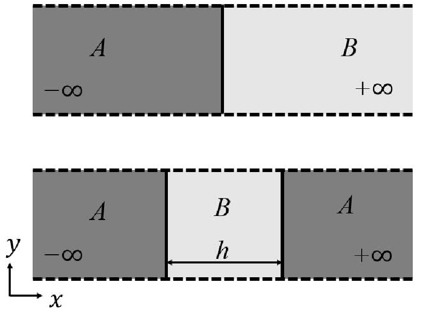
We then consider two flat interfaces, separated by a distance (see Fig. 3), now the integral in Eq. (15) is defined as the overall line tension,
| (16) |
As we can see, is a function of , and the limit condition is . According to Refs. [47, 25], the disjoining pressure is defined as
| (17) |
where . A simple differentiation of Eq. (17) yields . Supplementing with the boundary condition , the disjoining pressure finally reads as follows,
| (18) |
By setting a series of interface distances, Eq. (18) can be calculated using standard numerical integration method.
III NUMERICAL SIMULATIONS
In this section, numerical simulations are conducted to verify the aforementioned arguments and highlight the main features of the present two-range pseudopotential model. Unless otherwise specified, the strength coefficients in Eq. (8) are set the same for both components ( and ) with [25, 27], and the coefficients is chosen such that the interface width is about 4 lattice spacings [48].

III.1 Two-component Poiseuille flow
Firstly, a two-component Poiseuille flow (along the direction) driven by a body force is studied (see also Fig. 4). In this flowing system, the nonwetting phase (component ) flows in the central region of the channel, , the wetting phase (component ) flows between the nonwetting phase and the walls, , and the dynamic viscosity ratio is ( simplifies to the kinematic viscosity ratio due to the unit density ratio considered). In our simulations, periodic boundary conditions are applied along the direction, the half-way bounce-back boundary scheme is applied to the up and bottom walls, and the computational domain is covered by lattice nodes. The analytical solution for the problem is given by [48],
| (19) |
where the body force acts on both components and is set to , with .


It is known that the velocity shift forcing scheme suffers numerical instability for two-component flow with a relatively high kinematic viscosity ratio [49]. All implementations of the original two-range model so far were at [23, 24, 25]. Figure 5 shows the comparison between numerical results obtained with the present two-range model and the analytical solutions at different viscosity ratios, (from left to right). For the original two-range model, the simulation is unstable for , thus it is not shown in the figure. For the present model, we consider three cases: two of them corresponding to positive disjoining pressures ( and -8) and a reference case ( ). It can be seen that the numerical results are in good agreement with the analytical solutions, except for some small discrepancies near the interface. As analyzed in Refs. [48, 50], the small discrepancies may be related the diffused interface feature in LBM and have no significant effects on the flow away from the interface. These results prove that, with our model, the viscosity ratio can be tunable over a relatively large range, still reproducing physically correct results.
III.2 Tunable surface tension

In the single-range pseudopotential model, the surface tension can only be varied through the parameter . Thanks to the introduction of the competing mechanism, the surface tension in the present two-range model can be also adjusted by tuning the parameters and . To confirm this statement, a series of Laplace’s tests are carried out to measure the surface tension under different conditions. Four different cases (; ; and ) are considered, in which the first case corresponds to the classical single-range model. The tunable range of and the achievable range of are shown in Table 1. The parameter is tuned progressively with a 0.1 interval to find a range over which the measured interface thickness is within ; such range is costrained since too sharp interfaces () suffer from numerical instability and too wide ones () deteriorate the numerical accuracy near the interface. The interface width is defined by fitting a hyperbolic tangent curve to the density profile [34], which can be rewritten as with and solved using the finite difference method (see Fig. 6).
It can be seen from Table 1 that the achievable range for the single-range model is . For the two-range model, we have more freedom to tune the surface tension due to the additional competing interactions, and for the four cases considered in this work, the achievable range is . Specifically, larger (smaller) gives larger (smaller) surface tension, because, at fixed , the diagonal elements of the kinetic pressure tensor are proportional to (see Eqs. (14-16) in [24]).
In addition, unlike the original two-range model [24], where the surface tension is viscosity-dependent, in the present model the surface tension and viscosity ratio are decoupled, as it will be discussed in the next subsection.
| case | ||||
|---|---|---|---|---|
| range of | ||||
| range of |
III.3 Independence of surface tension and disjoining pressure on the viscosity ratio
The emergence of positive disjoining pressure is a unique feature of the two-range model, which supports the stable thin film between two interfaces and distinguishes the two-range model from the classical single-rang. To measure the disjoining pressure , we consider two planar interfaces, separated by a distance (see also Fig. 3). After is obtained through Eq. (16) for various ’s, the disjoining pressure can be calculated according to Eq. (18). To be general, we introduce a dimensionless disjoining pressure , where is a length scale defined as . Firstly, we choose , and calculate the dimensionless disjoining pressure as a function of the dimensionless distance for the present model with different pairs of , as shown in Fig. 7. From the figure, we can see that for the case (), corresponding to the classical single-range model, the disjoining pressure is always negative and decreases with . For other cases with the two-range competing interactions, the disjoining pressure increases with the decrease of firstly and then goes down, attaining positive values inbetween.


Then we compare the original two-range [23, 24] and the present model in Fig. 8. For the original model, some -dependent terms are reproduced in (see Eq. (14)), thus the surface tension is dependent on the viscosity for each component. In this simulation, the measured surface tensions at viscosity ratio are 0.056, 0.043 and 0.039, respectively. Remarkably, the -dependent terms in are removed by using the present forcing scheme. Under different viscosity ratio , the surface tension is approximately constant (with a maximum relative error of ). As a result, the disjoining pressure depends on significantly for the original model in Refs. [23, 24], while it is independent of for the present model. To highlight this point, we consider collisions of droplets of component in a liquid matrix of component . We wish to point out that the configuration here is consistent with Fig. 3, because a thin film (component ) is produced between the two droplets (component ) when the two droplets are approaching each other. Two equal-sized droplets with a diameter are initialized with a relative velocity , which leads to a Capillary number and a Weber number . First, we choose a unity viscosity ratio . Due to the positive disjoining pressure, a stable thin film between the droplets is supported, and the two droplets bounce back in the end, as shown in Fig. 9. Then we change to 0.3. For the present model, the disjoining pressure is viscosity-independent, thus the two droplets still bounce back in Fig. 10. However, the disjoining pressure changes to negative for the original model when . As a result, the thin film cannot be supported any longer, and the two droplets eventually coalesce.
The novelty of the present model, which displays a disjoining pressure independent of the viscosity ratio, represents a significant improvement with respect to the original model and makes it of major significance for many applications where non unit viscosity ratios are needed [51, 52, 53, 54, 55, 56].


(a)


(b)


(a)


(b)
III.4 Pressure-driven emulsion in a planar channel
The method we have presented, thanks to its built-in properties, results particularly suitable to simulate the hydrodynamics of emulsions, especially in dense situations. We move therefore here to simulate a multi-droplet situation. We consider a pressure-driven flow in a planar channel of a monodisperse emulsion, made of a regular arrangement of equal size droplets (component ) dispersed in a continuous matrix (component ). The simulations are performed on a domain, with ; no-slip boundary conditions for the velocity are imposed on the top () and bottom () walls; non-wetting boundary conditions for droplets apply, i.e. a contact angle of is set for component on both walls. A body force in the -direction is imposed to mimic a constant pressure gradient, which can be expressed in non-dimensional form as (let us notice that such expression coincides with the Reynolds number that would be achieved in the corresponding Poiseuille flow in the pure continuous phase, for that given forcing ). The coupling parameters are , , , giving , and the droplet radius is set within to obtain different volume fractions of the dispersed phase, (typical snapshots of are shown in Fig. 11).


When no droplets are present in the system (), the usual Poiseuille flow profile for a pure fluid is obtained, as shown in the left panel of Fig. 12. In Fig. 12, left panel, we show the velocity profile for different volume fractions at and , where is the average velocity along direction. As expected, when is increased, the velocity profile flattens gradually in the central region of the channel, which is consistent with previous results [25, 54]. To quantify the effect of increasing the volume fraction, we estimate the relative effective viscosity as the ratio of flow rates , where . A plot of as a function of at is shown in the right panel of Fig. 12. It can be seen that the relative effective viscosity increases nonlinearly with , as observed also for a similar system with neutral wetting boundaries for the droplets [54]. A number of expressions for the effective viscosity of an emulsion as a function of the volume fraction are available in the literature [57, 58]. Based on the differential effective medium theory, Bullard et al. [58] proposed the following model,
| (20) |
where the factor is set to be , and represent the intrinsic viscosity. For the present system with slightly deformable droplets (see Fig. 11), the intrinsic viscosity is restricted between the undeformable limit of Taylor [59] and the freely deformable limit of Douglas et al. [60] , where . In Fig. 12, we show a very good fit by Eq. (20) with


We now proceed to investigate the effect of body force by exploring a range of non-dimensional body forces . Figure. 13 plots as a function of at different volume fractions. From Fig. 13, we can see that is almost independent of the forcing in the parameter range we considered, as expected for a Newtonian fluid. For the highest volume fraction tested, , instead, a slight decrease of with the increasing forcing can be appreciated, hinting at a moderate shear thinning behaviour, as expectable for this kind of systems.

We address now the effect of the viscosity ratio on the rheology of the emulsion. We stress, here, incidentally that the capability of simulating viscosity ratios other than one extends the applicability of our method to study the physics of more general soft flowing systems. In this sense, the limit is that of suspensions, while would correspond to foams. In Fig. 14 we plot the relative effective viscosity as a function of the viscosity ratio . We can see an asymmetric effect of : for , is approximately independent of , while for , increases with the decrease of and this effect is more significant at larger volume fractions. As shown in the inset, we also find good fits by Eq. (20) for , where the intrinsic viscosity in each fitting line is restricted between and for the specified condition.

IV Conclusions
A mesoscopic numerical method for the simulation of soft flowing systems based on a two-range pseudopotential lattice Boltzmann has been proposed. Our method is unique as it features adjustable surface tension, positive disjoining pressure, tunable viscosity ratio and fully resolved hydrodynamics, unlike any other existing alternative (such as boundary integral methods [61] or “bubble models” [62]). In contrast to the previous literature, the present model removes the viscosity-dependence in the original two-range pseudo-potential LBM, thus opening the way to the simulation of multicomponent fluids with non-unit viscosity ratios and a viscosity-independent disjoining pressure. Such capability is demonstrated by computing the relative effective viscosity of a pressure-driven emulsion in a planar flow as a function of the viscosity ratio between the disperse and continuum phases.
It is hoped that the present upgrade will permit to extend the range of applications of the LBM for complex soft-flowing systems.
Acknowledgements.
The authors thank Prof. Mauro Sbragaglia and Prof. Anthony Ladd for fruitful discussions. The research leading to these results has received funding from the MOST National Key Research and Development Programme (Project No. 2016YFB0600805), the European Research Council under the European Union’s Horizon 2020 Framework Programme(No. FP/2014-2020)/ERC Grant Agreement No. 739964 (“COPMAT”), and the China Scholarship Council (CSC, No. 201706210262). Supercomputing time on ARCHER is provided by the “UK Consortium on Mesoscale Engineering Sciences (UKCOMES)” under the UK Engineering and Physical Sciences Research Council Grant No. EP/R029598/1.Appendix A Spurious currents
It is known that the diffusive interface models lead to spurious velocity currents around interfaces due to the numerical imbalances of various discretized forces. The maximum spurious currents, , produced for a steady droplet ( ) under different conditions are shown in Fig. 15. The parameters used in the simulations are the same as those in Sec. III.4. As can be seen, the maximum spurious current is relatively small for viscosity ratio (the range considered in Sec. III.4), while it increases gradually when is further decreased. For a given viscosity ratio, is reduced when the strength coefficient is increased, which corresponds to smaller disjoining pressure (see Fig. 7). For the time being, we mainly focus on the removal of the viscosity-dependence in the original two-range model, while strategies or parameter optimization methods [10, 63, 64, 55] for reducing the spurious currents can be adopted for future applications with quite small (or quite large) viscosity ratios.

References
- [1] R.G. Larson, The Structure and Rheology of Complex Fluids, Topics in Chemical Engineering (OUP USA, 1999).
- [2] Johannes Lyklema, Fundamentals of interface and colloid science: soft colloids, Vol. 5 (Elsevier, 2005).
- [3] Philippe Coussot, Rheometry of pastes, suspensions, and granular materials: applications in industry and environment (John Wiley & Sons, 2005).
- [4] Denis L Weaire and Stefan Hutzler, The physics of foams (Oxford University Press, 2001).
- [5] Shelley L Anna and Hans C Mayer, “Microscale tipstreaming in a microfluidic flow focusing device,” Physics of Fluids 18, 121512 (2006).
- [6] Haihu Liu and Yonghao Zhang, “Droplet formation in microfluidic cross-junctions,” Physics of Fluids 23, 082101 (2011).
- [7] Yuhang Fu, Lin Bai, Yong Jin, and Yi Cheng, “Theoretical analysis and simulation of obstructed breakup of micro-droplet in t-junction under an asymmetric pressure difference,” Physics of Fluids 29, 032003 (2017).
- [8] Ashish Bhateja and Devang V Khakhar, “Rheology of dense granular flows in two dimensions: Comparison of fully two-dimensional flows to unidirectional shear flow,” Physical Review Fluids 3, 062301 (2018).
- [9] Peter Sollich, François Lequeux, Pascal Hébraud, and Michael E Cates, “Rheology of soft glassy materials,” Physical review letters 78, 2020 (1997).
- [10] Qing Li, Kai Hong Luo, QJ Kang, YL He, Q Chen, and Q Liu, “Lattice boltzmann methods for multiphase flow and phase-change heat transfer,” Progress in Energy and Combustion Science 52, 62–105 (2016a).
- [11] Guy R McNamara and Gianluigi Zanetti, “Use of the boltzmann equation to simulate lattice-gas automata,” Physical review letters 61, 2332 (1988).
- [12] Gerhard Besold, Ilpo Vattulainen, Mikko Karttunen, and James M Polson, “Towards better integrators for dissipative particle dynamics simulations,” Physical Review E 62, R7611 (2000).
- [13] YH Qian, Dominique d’Humières, and Pierre Lallemand, “Lattice bgk models for navier-stokes equation,” EPL (Europhysics Letters) 17, 479 (1992).
- [14] Roberto Benzi, Sauro Succi, and Massimo Vergassola, “The lattice boltzmann equation: theory and applications,” Physics Reports 222, 145–197 (1992).
- [15] Xiaowen Shan and Hudong Chen, “Lattice boltzmann model for simulating flows with multiple phases and components,” Physical Review E 47, 1815 (1993).
- [16] Massimo Bernaschi, Massimiliano Fatica, Simone Melchionna, Sauro Succi, and Efthimios Kaxiras, “A flexible high-performance lattice boltzmann gpu code for the simulations of fluid flows in complex geometries,” Concurrency and Computation: Practice and Experience 22, 1–14 (2010).
- [17] Zhaoli Guo and Chang Shu, Lattice Boltzmann method and its applications in engineering, Vol. 3 (World Scientific, 2013).
- [18] Sauro Succi, “Lattice boltzmann 2038,” EPL (Europhysics Letters) 109, 50001 (2015).
- [19] Sauro Succi, The Lattice Boltzmann Equation: For Complex States of Flowing Matter (Oxford University Press, 2018).
- [20] Linlin Fei, Kai Hong Luo, Chuandong Lin, and Qing Li, “Modeling incompressible thermal flows using a central-moments-based lattice boltzmann method,” International Journal of Heat and Mass Transfer 120, 624–634 (2018a).
- [21] Marco Lauricella, Simone Melchionna, Andrea Montessori, Dario Pisignano, Giuseppe Pontrelli, and Sauro Succi, “Entropic lattice boltzmann model for charged leaky dielectric multiphase fluids in electrified jets,” Physical Review E 97, 033308 (2018).
- [22] Giacomo Falcucci, Gino Bella, Giancarlo Chiatti, Sergio Chibbaro, Mauro Sbragaglia, and Sauro Succi, “Lattice boltzmann models with mid-range interactions,” Commun. Comput. Phys 2, 1071–1084 (2007).
- [23] Roberto Benzi, Sergio Chibbaro, and Sauro Succi, “Mesoscopic lattice boltzmann modeling of flowing soft systems,” Physical review letters 102, 026002 (2009a).
- [24] Roberto Benzi, Mauro Sbragaglia, Sauro Succi, Massimo Bernaschi, and Sergio Chibbaro, “Mesoscopic lattice boltzmann modeling of soft-glassy systems: theory and simulations,” The Journal of Chemical Physics 131, 104903 (2009b).
- [25] M Sbragaglia, R Benzi, M Bernaschi, and S Succi, “The emergence of supramolecular forces from lattice kinetic models of non-ideal fluids: applications to the rheology of soft glassy materials,” Soft Matter 8, 10773–10782 (2012).
- [26] R Benzi, M Sbragaglia, A Scagliarini, P Perlekar, M Bernaschi, S Succi, and F Toschi, “Internal dynamics and activated processes in soft-glassy materials,” Soft Matter 11, 1271–1280 (2015).
- [27] Benjamin Dollet, A Scagliarini, and M Sbragaglia, “Two-dimensional plastic flow of foams and emulsions in a channel: experiments and lattice boltzmann simulations,” Journal of Fluid Mechanics 766, 556–589 (2015).
- [28] Andrea Scagliarini, Benjamin Dollet, and Mauro Sbragaglia, “Non-locality and viscous drag effects on the shear localisation in soft-glassy materials,” Colloids and Surfaces A: Physicochemical and Engineering Aspects 473, 133–140 (2015).
- [29] Zhaoli Guo, Chuguang Zheng, and Baochang Shi, “Discrete lattice effects on the forcing term in the lattice boltzmann method,” Physical Review E 65, 046308 (2002).
- [30] Xiaowen Shan and Gary Doolen, “Multicomponent lattice-boltzmann model with interparticle interaction,” Journal of Statistical Physics 81, 379–393 (1995).
- [31] Xiaowen Shan and Hudong Chen, “Simulation of nonideal gases and liquid-gas phase transitions by the lattice boltzmann equation,” Physical Review E 49, 2941 (1994).
- [32] Haibo Huang, Manfred Krafczyk, and Xiyun Lu, “Forcing term in single-phase and shan-chen-type multiphase lattice boltzmann models,” Physical Review E 84, 046710 (2011).
- [33] Q Li, Kai Hong Luo, and X J Li, “Forcing scheme in pseudopotential lattice boltzmann model for multiphase flows,” Physical Review E 86, 016709 (2012).
- [34] Daniel Lycett-Brown and Kai H Luo, “Improved forcing scheme in pseudopotential lattice boltzmann methods for multiphase flow at arbitrarily high density ratios,” Physical Review E 91, 023305 (2015).
- [35] Xiaoyi He, Shiyi Chen, and Gary D Doolen, “A novel thermal model for the lattice boltzmann method in incompressible limit,” Journal of Computational Physics 146, 282–300 (1998a).
- [36] Xiaoyi He, Xiaowen Shan, and Gary D Doolen, “Discrete boltzmann equation model for nonideal gases,” Physical Review E 57, R13 (1998b).
- [37] Paul J Dellar, “An interpretation and derivation of the lattice boltzmann method using strang splitting,” Computers & Mathematics with Applications 65, 129–141 (2013).
- [38] Farzaneh Hajabdollahi and Kannan N Premnath, “Symmetrized operator split schemes for force and source modeling in cascaded lattice boltzmann methods for flow and scalar transport,” Physical Review E 97, 063303 (2018).
- [39] Q Li, P Zhou, and HJ Yan, “Revised chapman-enskog analysis for a class of forcing schemes in the lattice boltzmann method,” Physical Review E 94, 043313 (2016b).
- [40] Linlin Fei and Kai Hong Luo, “Consistent forcing scheme in the cascaded lattice boltzmann method,” Physical Review E 96, 053307 (2017).
- [41] Rongzong Huang, Huiying Wu, and Nikolaus A Adams, “Eliminating cubic terms in the pseudopotential lattice boltzmann model for multiphase flow,” Physical Review E 97, 053308 (2018).
- [42] Linlin Fei, Kai H Luo, and Qing Li, “Three-dimensional cascaded lattice boltzmann method: Improved implementation and consistent forcing scheme,” Physical Review E 97, 053309 (2018b).
- [43] Giacomo Falcucci, Stefano Ubertini, and Sauro Succi, “Lattice boltzmann simulations of phase-separating flows at large density ratios: the case of doubly-attractive pseudo-potentials,” Soft Matter 6, 4357–4365 (2010).
- [44] Xiaowen Shan, “Pressure tensor calculation in a class of nonideal gas lattice boltzmann models,” Physical Review E 77, 066702 (2008).
- [45] M Sbragaglia and D Belardinelli, “Interaction pressure tensor for a class of multicomponent lattice boltzmann models,” Physical Review E 88, 013306 (2013).
- [46] BV Derjaguin and NV Churaev, “On the question of determining the concept of disjoining pressure and its role in the equilibrium and flow of thin films,” Journal of Colloid and Interface Science 66, 389–398 (1978).
- [47] Vance Bergeron, “Forces and structure in thin liquid soap films,” Journal of Physics: Condensed Matter 11, R215 (1999).
- [48] Mark L Porter, E T Coon, Q Kang, J D Moulton, and J W Carey, “Multicomponent interparticle-potential lattice boltzmann model for fluids with large viscosity ratios,” Physical Review E 86, 036701 (2012).
- [49] Haibo Huang, Michael Sukop, and Xiyun Lu, Multiphase lattice Boltzmann methods: Theory and application (John Wiley & Sons, 2015).
- [50] Qiuxiang Li, Zhenhua Chai, Baochang Shi, and Hong Liang, “Deformation and breakup of a liquid droplet past a solid circular cylinder: A lattice boltzmann study,” Physical Review E 90, 043015 (2014).
- [51] Thomas Cubaud and Thomas G Mason, “Capillary threads and viscous droplets in square microchannels,” Physics of Fluids 20, 053302 (2008).
- [52] H Farhat and JS Lee, “Suppressing the coalescence in the multi-component lattice boltzmann method,” Microfluidics and nanofluidics 11, 137–143 (2011).
- [53] Lin Bai, Yuhang Fu, Shufang Zhao, and Yi Cheng, “Droplet formation in a microfluidic t-junction involving highly viscous fluid systems,” Chemical Engineering Science 145, 141–148 (2016).
- [54] M. Foglino, A. N. Morozov, O. Henrich, and D. Marenduzzo, “Flow of deformable droplets: discontinuous shear thinning and velocity oscillations,” Physical review letters 119, 208002 (2017).
- [55] Andrea Montessori, Marco Lauricella, Michele La Rocca, Sauro Succi, Elad Stolovicki, Roy Ziblat, and David Weitz, “Regularized lattice boltzmann multicomponent models for low capillary and reynolds microfluidics flows,” Computers & Fluids 167, 33–39 (2018).
- [56] Elad Stolovicki, Roy Ziblat, and David A Weitz, “Throughput enhancement of parallel step emulsifier devices by shear-free and efficient nozzle clearance,” Lab on a Chip 18, 132–138 (2018).
- [57] Svetlana R Derkach, “Rheology of emulsions,” Advances in colloid and interface science 151, 1–23 (2009).
- [58] Jeffrey W Bullard, Adam T Pauli, Edward J Garboczi, and Nicos S Martys, “A comparison of viscosity–concentration relationships for emulsions,” Journal of colloid and interface science 330, 186–193 (2009).
- [59] Geoffrey I Taylor, “The viscosity of a fluid containing small drops of another fluid,” Proceedings of the Royal Society of London. Series A 138, 41–48 (1932).
- [60] Jack F Douglas and Edward J Garboczi, “Intrinsic viscosity and the polarizability of particles having a wide range of shapes,” Advances in chemical physics 91, 85–154 (1995).
- [61] M Loewenberg and EJ Hinch, “Numerical simulation of a concentrated emulsion in shear flow,” Journal of Fluid Mechanics 321, 395–419 (1996).
- [62] Douglas J Durian, “Foam mechanics at the bubble scale,” Physical review letters 75, 4780 (1995).
- [63] Daniel Lycett-Brown and Kai H Luo, “Multiphase cascaded lattice boltzmann method,” Computers & Mathematics with Applications 67, 350–362 (2014).
- [64] Daniel Lycett-Brown, Kai H Luo, Ronghou Liu, and Pengmei Lv, “Binary droplet collision simulations by a multiphase cascaded lattice boltzmann method,” Physics of Fluids 26, 023303 (2014).