An embedded SDG method for the convection-diffusion equation
Abstract
In this paper, we present an embedded staggered discontinuous Galerkin method for the convection-diffusion equation. The new method combines the advantages of staggered discontinuous Galerkin (SDG) and embedded discontinuous Galerkin (EDG) method, and results in many good properties, namely local and global conservations, free of carefully designed stabilization terms or flux conditions and high computational efficiency. In applying the new method to convection-dominated problems, the method provides optimal convergence in potential and suboptimal convergence in flux, which is comparable to other existing DG methods, and achieves stability by making use of a skew-symmetric discretization of the convection term, irrespective of diffusivity. We will present numerical results to show the performance of the method.
1 Introduction
Discontinuous Galerkin (DG) methods were first introduced by Reed and Hill for solving hyperbolic equations [40]. The DG methods have been proven superior to the classical continuous Galerkin (CG) methods for hyperbolic problems. In the past two decades, DG methods have also been applied to second-order elliptic problems. A comprehensive study on DG methods for elliptic problems is given in [1]. The original DG methods for elliptic problems, using polynomial approximations of degree for both the potential and the flux, converge with optimal order for the potential but suboptimal order for the flux. While the same orders of convergence can be obtained by using classical CG finite element methods, the DG methods give rise to a discrete problem with a higher number of degrees of freedom. DG methods have therefore been criticized for its high computation cost and judged to be not being particularly useful for elliptic problems. Later, the hybridizible discontinuous Galerkin (HDG) method was introduced for solving elliptic problems [23]. The HDG method provides optimal orders of convergence for both the potential and the flux in norm. Moreover, superconvergence can be obtained for the potential through a local postprocessing technique.
In recent years, there are active developments of DG methods for problems in fluid dynamics and wave propagations, see for example [6, 22, 24, 27, 28, 32, 36, 41, 42, 37]. On the other hand, staggered meshes bring the advantages of reducing numerical dissipation in computational fluid dynamics [2, 3, 31], and numerical dispersion in computational wave propagation [9, 10, 11, 12, 13, 14, 17]. Combining the ideas of DG methods and staggered meshes, a new class of staggered discontinuous Galerkin (SDG) methods was proposed for approximations of Stokes system [34], convection-diffusion equation [19], and incompressible Navier-Stokes equations [7]. The new class of SDG methods possesses many good properties, including local and global conservations, stability in energy, and optimal convergence. For a more complete discussion on the SDG method, see also [11, 12, 13, 14, 18, 19, 35] and the references therein.
In [15, 16], it was shown that the SDG method can be regarded as a limit of the HDG method. The SDG method can be obtained from the HDG method by setting the stabilization parameter on a set of edges to be zero and letting the parameter on another set of edges to infinity. As a result, the SDG method inherits the advantages of the HDG method, including superconvergence through the use of a local postprocessing technique. Furthermore, in the SDG method for incompressible Navier-Stokes equations [7], using the postprocessing and a spectro-consistent discretizations with a novel splitting of the diffusion and the convection term, stability in energy is achieved.
The embedded discontinuous Galerkin (EDG) method was first introduced for solving the linear shell problems [30]. Later, an EDG method for solving second order elliptic problems was discussed and analyzed in [26]. The EDG method was obtained from HDG method by enforcing strong continuity for hybrid unknowns [23]. This greatly reduces the number of degrees of freedom in the globally coupled system and makes the EDG method has a higher computational efficiency compared with other DG methods. As a tradeoff for this advantage, the EDG method is not locally conservative and loses the optimal convergence in the flux achieved by the HDG method [38]. The loss in accuracy makes the EDG method a less attractive candidate compared with the HDG method. However, the optimal order of convergence for HDG method is also lost in the case of convection-dominated problems as shown the numerical examples [25]. In this case, the EDG method becomes appealing alternative to all other DG methods including the HDG method, since it has a higher computational efficiency and the same orders of convergence. On the other hand, compared with the CG finite element method, the EDG method provides the same sparsity structure of the stiffness matrix after static condensation, whilist the EDG method is more robust, accurate and stable than the CG finite element method in convection-dominated problems. We remark that the multiscale discontinuous Galerkin (MDG) method [5, 33] are related to the EDG method, which is originally proposed for the convection-diffusion problems. The MDG method and the EDG method are both designed for a globally continuous approximation of the solution and can give rise to identical schemes. Recently, the EDG method has been proposed on Euler equations and Navier-Stokes equations [38, 39]. Due to the advantages shared with other DG methods and the high computational efficiency compared with other DG methods, the EDG method has also been applied to challenging problems in computational fluid dynamics, such as implicit large eddy simulation [29].
In this paper, we propose a combination of the SDG method and the EDG method for the convection-diffusion equation. The new method seeks approximations in the SDG locally conforming finite element spaces, which gives rise to a flux formulation without introducing any carefully designed stabilization terms or flux conditions as in other DG methods. The new method further reduces the size of the global discrete problem compared with SDG method by restricting the numerical approximation for the primal unknown to lie in a proper subspace of the SDG finite element space. Moreover, the new method inherits the stability in energy thanks to spectro-consistent discretizations in the SDG method. The convergence is optimal with order for the unknown function and suboptimal with order for its gradient, which are comparable to all other DG methods for convection-dominated problems.
2 Method description
2.1 Model problem
Let be a polygonal domain. We consider the steady-state convection-diffusion equation with homogeneous Dirichlet boundary condition:
| (1) |
Here is the unknown function to be approximated, is a divergence-free convection field, is a given source term and is a given boundary condition. Also, is the diffusivity, which is assumed to be constants throughout the domain . Before we start the derivation of our method, we shall state the variational formulation of the problem. Suppose and . The variational formulation of the convection-diffusion equation is given by: find such that for any , we have
| (2) |
Here denotes the standard inner product.
2.2 Staggered meshes
Let be a triangulation of the two-dimensional domain by a set of triangles without hanging nodes. We introduce the notation to denote the set of all edges in the triangulation and to denote the subset of all interior edges in excluding those on the boundary of . We also denote the set of all vertices in by . For each triangle in , we take an interior point , denote the initial triangle by , and divide into three triangles by joining the point and the three vertices of . We also denote the set of all interior points by , the set of all new edges generated by the subdivision of triangles by , and the triangulation after subdivision by . Note that the interior point of each triangle in should be chosen such that the new triangulation observes the shape regularity criterion. In practice, we can simply choose as the centroid of the triangle. Also, denotes the set of all edges of triangles in and denotes the set of all interior edges of triangles in . For each edge , we let be the union of the all triangles in the new triangulation sharing the edge . Figure 1 demonstrates these definitions. The edges are represented in solid lines and the are represented in dotted lines.

For each edge , we will also define a unit normal vector in the following way. If is a boundary edge, then we define as the outward unit normal vector of from . If is an interior edge, then is fixed as one of the two possible unit normal vectors on . When it is clear that which edge we are considering, we omit the index and write the unit normal vector as .
To end this section, we define the jumps in the following way: for any edge , denote one of the triangles in the refined triangulation , which contains by , and denote the other triangle, if exists, by . The outward unit normal vectors on in and are denoted by and , respectively. Also, for any quantity , the notations are defined on the edge by the values of restricted on . Then, if is a scalar quantity, the notation over an edge defined as
| (7) |
If is a vector quantity, then the notation is similarly defined as
| (8) |
2.3 SDG and ESDG finite element spaces
We will define the finite element spaces. Let be a non-negative integer. Let and . We define and as the space of polynomials whose order is not greater than on and , respectively. We will also define norms on the spaces. We use the standard notations to denote the standard norm on and to denote the norm on an edge .
First, we define the following locally -conforming finite element space:
| (9) |
Note that for any , we have for each edge . We define the following discrete -norm and discrete -norm on the space :
| (10) |
Next, we define the following ESDG finite element space, which is a proper subspace of the SDG finite element space:
| (11) |
Note that the test functions are continuous at only all the nodes in the initial grid but not the nodes at the refined grid, are therefore they are not globally continuous. We remark that for the EDG method [26], the space of the numerical trace is imposed with a global continuity on the skeleton of the mesh.
2.4 Derivation of the method
We will derive the discrete problem in our SDG formulation starting from the system of first order equations in (5) and (6).
Multiplying the first equation of (5) by and integrating over for , we obtain
| (16) |
Similarly, multiplying the second equation of (5) by and integrating over for , we have
| (17) |
Finally, multiplying the first equation of (6) by and integrating over for , we have
| (18) |
Summing those equations in (16)–(18) over all and , we obtain the staggered discontinuous Galerkin method for (1) proposed in [19]: find such that for any , we have
| (19) |
where bilinear forms and are defined as
| (20) |
and the bilinear forms and are defined as
| (21) |
Now, if we consider only the test functions in (18), and we seek an approximation for the unknown function , we obtain the embedded staggered discontinuous Galerkin method for (1): find such that for any , we have
| (22) |
By [12], the two bilinear forms in (20) satisfy the adjoint relation
| (23) |
for all and . The bilinear forms and are also continuous with respect to suitable discrete norms
| (24) |
for all and . Moreover, the bilinear forms and satisfy a pair of inf-sup conditions: there exists constants and , independent of , such that
| (25) |
2.5 Linear system
In this section, we derive the linear systems resulting from (19) and (22). We denote the corresponding matrix representation of the bilinear forms and by and , respectively. Then by the adjoint properties, the matrix representation of the bilinear forms and are given by and , respectively. Also, the notations for the finite element solutions would be abused to denote their corresponding vector representations.
Using these notations, we can write the SDG method (19) as a linear system of algebraic equations. The second equation of (19) can be written as
| (27) |
where is the mass matrix for the space . Similarly, the last equation of (19) can be written as
| (28) |
Lastly, the first equations of (19) can be written as
| (29) |
We can now obtain a linear system with the unknowns and eliminated. Combining (27) and (28), we have
| (30) |
We note that the elimination can be done by solving small problems in each since is a block diagonal matrix with each block corresponding to the mass matrix of .
We further introduce the notations
| (31) |
We note that the discrete diffusion operator is symmetric and positive-definite, and the discrete convection operator is skew-symmetric. Combining (29) and (30), the algebraic system of the discrete problem (19) can then be reduced to
| (32) |
Now, if we denote the matrix representation of the canonical embedding by , then the matrix representations and of the bilinear forms and are related to and by
| (33) |
The corresponding matrix represenations for the discrete diffusion operator and discrete convection operator are
| (34) |
Therefore the algebraic system of the discrete problem (22) is given by
| (35) |
where
| (36) |
We remark that in the embedded SDG method, the discretization of the diffusion operator is still symmetric and positive definite. Similarly, the discretization of the convection operator is still skew-symmetric. Therefore the spectro-consistent discretization is preserved in the new method.
3 Stability analysis
We start this section by stating a stability result in energy for the variational formulation (2).
Lemma 3.1.
Let be the weak solution of the variational formulation (2) of the convection-diffusion equation. Then we have
| (37) |
We will next see that the ESDG method provides a similar stability result. In the SDG method, the stability in energy is due to a spectro-consistent discretizations with the splitting of the diffusion and the convection term proposed in [19]. The stability in energy in a numerical method for the convection-diffusion problems is a kind of measure of how well the numerical solution approximates the analytical solution, and has significant effects on the quality of the numerical solution (see, for example, [7], [8]; also see Section 5.3). The ESDG method inherits the stability in energy from the SDG method due to the same spectro-consistent discretization structure.
The unknowns in the space in both the SDG method and the ESDG method give rise to an approximation of the flux in the space . For the ESDG method, suppose is the solution of (22). An approximation for the flux is then given by
| (40) |
Likewise for the SDG method, suppose is the solution of (19). An approximation for the flux is given by
| (41) |
We are now ready to state the stability result for the ESDG method:
Lemma 3.2.
An important message from Lemma 3.2 is that the convection field vanishes in the above stability estimate for . This makes the ESDG approximation mimics the weak solution better as the convection field also vanishes in the above stability estimate for in Lemma 3.1. This is an advantage brought by the novel splitting of the convection term and the diffusion term.
To end this section, we establish the main stability result.
Theorem 3.3.
Let be the numerical solution of the ESDG method (22). Then we have
| (47) |
where is a constant independent of mesh size and diffusivity.
Proof.
By Lemma 3.2, we have
| (48) |
By Cauchy-Schwarz inequality and the equivalence of the standard norm and the discrete norm on the finite dimensional space , we obtain the following estimate for the right hand side:
| (49) |
where is the constant from the equivalence of norms. On the other hand, by the adjoint relation (23) and the first inf-sup condition in (25), we have
| (50) |
Therefore we have
| (51) |
Dividing on both sides, we obtain the desired result. ∎
4 Convergence analysis
In this section, we present an error estimate between the weak solution in (6) and the ESDG solution in (22).
Theorem 4.1.
Let be the solution of (5)–(6). Let be the numerical solution of the ESDG method (22). Then we have the following optimal error bound:
| (52) |
where is a constant independent of mesh size and diffusivity.
Proof.
First, we note that the solution satisfies the following system:
| (53) |
for any . Subtracting (22) from (53), we have
| (54) |
Introduce the notations
| (55) |
Using the properties in (14), we can rewrite (54) as
| (56) |
Using the argument as in (50), by the second equation in (56), we have
| (57) |
Moreover, using a discrete Poincaré inequality, we have
| (58) |
On the other hand, in (56), we take we take test functions as follows:
| (59) |
Then we have
| (60) |
Summing up the equations in (60) and using the adjoint relations (23) and (26), we have
| (61) |
where
| (62) |
Next, we will estimate each of these terms. Using Young’s inequality, we have
| (63) |
Similarly, for , we imply
| (64) |
For , we have
| (65) |
For , we first observe that
| (66) |
Taking in the last equation of (56), we have
| (67) |
Hence we imply
| (68) |
Combining all these estimates with (61), we have
| (69) |
Combining (58) and (69), we have
| (70) |
Therefore, we have
| (71) |
Finally, using the approximation properties (15), we imply
| (72) |
Using triangle inequality on , we obtain our desired result. ∎
We remark that the error consists of two parts. The difference between the numerical solution and the interpolation image depends on the viscosity coefficient , while the interpolation error does not. As we will see in our numerical results, the error does not vary significantly with the viscosity coefficient .
5 Numerical results
In this section, we illustrate some numerical examples. We carry out numerical experiments to see and compare the rates of convergence of the SDG method and the ESDG method. Polynomials with degree is used for SDG approximations. We are interested in the error of the unknown function and also that of the flux . We recall the definitions in (40) and (41) for numerical approximations of the flux.
Throughout this section, we will take and use a family of staggered meshes in all the experiments. We denote the number of uniform divisions in in the mesh by . The domain is partitioned into sub-squares with length . Each sub-square is then divided into two identical right-angled triangles by its diagonal. This constructs the initial triangulation . To construct the staggered mesh , we simply take the interior point as the centroid in each initial triangle . Figure 2 illustrates a member of this family with . Table 1 compares the numbers of degrees of freedom in the discrete problems (32) for the SDG method and (35) for the ESDG method for this family of mesh. It can be seen that the number of degrees of freedom for the ESDG method is almost half of that of the SDG method for each level of mesh. Indeed, it can be worked out that for this family of mesh, the ratio of the numbers of the degrees of freedom is asymptotically:
| (73) |

| 2 | 56 | 33 |
|---|---|---|
| 4 | 208 | 121 |
| 8 | 800 | 465 |
| 16 | 3136 | 1825 |
| 32 | 12416 | 7233 |
| 64 | 49408 | 28801 |
5.1 Experiment 1: comparison to the EDG method
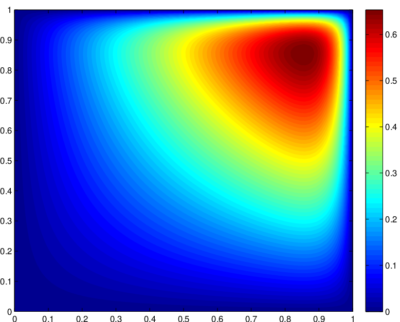
The purpose of this experiment is to compare our method with [38] in the same setting. In this experiment, the convection field is a constant vector. The analytic solution of this experiment is given by
| (74) |
For large values of and , there is a boundary layer around the segments and . The diffusivity are set to be . The constant convection field is chosen to be and the problem is weakly convection-dominated. A homogeneous Dirichlet boundary condition is prescribed. The source function is computed accordingly. The SDG method (19) and the ESDG method (22) are used to solve the problem numerically. We examine the performance of the ESDG method by comparing the errors and the orders of convergence to the EDG method and the SDG method.
Figure 3 shows a plot of the numerical solution of the ESDG method. Tables 2 compare the convergence results of the SDG method and the ESDG method with various scales of diffusivity . The second to the firth columns record the error and the orders of convergence of the potential and the flux for the SDG method. The sixth to the ninth columns record the error and the orders of convergence of the potential and the flux for the ESDG method. It can be seen that the approximated potential converge with an optimal order in error for both the SDG method and the ESDG method, which is the same for the EDG method in [38]. In particular, for and , the ESDG method gives a error smaller that the SDG method and also the EDG method. However, similar to the EDG method for second-order elliptic problems [26], our numerical results show that the ESDG method only provides a suboptimal order of convergence of error of the approximated flux, while the SDG method provides an optimal order .
| Mesh | ||||||||
|---|---|---|---|---|---|---|---|---|
| Error | Order | Error | Order | Error | Order | Error | Order | |
| 2 | 1.50e-01 | – | 2.48e+00 | – | 1.03e-01 | – | 2.31e+00 | – |
| 4 | 8.42e-02 | 0.84 | 1.63e+00 | 0.60 | 5.80e-02 | 0.82 | 2.00e+00 | 0.21 |
| 8 | 3.37e-02 | 1.32 | 6.96e-01 | 1.23 | 2.23e-02 | 1.38 | 1.38e+00 | 0.54 |
| 16 | 1.03e-02 | 1.72 | 2.15e-01 | 1.70 | 6.15e-03 | 1.86 | 7.92e-01 | 0.80 |
| 32 | 2.72e-03 | 1.91 | 5.71e-02 | 1.91 | 1.55e-03 | 1.99 | 4.13e-01 | 0.94 |
| 64 | 6.91e-04 | 1.98 | 1.45e-02 | 1.98 | 3.86e-04 | 2.00 | 2.09e-01 | 0.98 |
5.2 Experiment 2: sensitivity of orders of convergence to diffusivity
The purpose of this experiment is to examine the performance of the ESDG method in terms of convergence and compare the ESDG method with the SDG method in various scales of diffusivity. In this experiment, the convection field is set to be
| (75) |
The analytic solution of this experiment is given by
| (76) |
Figure 4 shows a plot of the convection field in this experiment. We perform the experiment with different scales of diffusivity . In particular, we are interested in observing the behaviour of the solutions when is small, i.e. the problem is convection-dominated. An inhomogeneous Dirichlet boundary condition is prescribed. The source function is computed accordingly. The SDG method (19) and the ESDG method (22) are used to solve the problem numerically. We examine the performance of the ESDG method by comparing the errors and the orders of convergence to the SDG method.

Tables 3–9 compare the convergence results of the SDG method and the ESDG method with various scales of diffusivity . The second to the firth columns record the error and the orders of convergence of the potential and the flux for the SDG method. The sixth to the ninth columns record the error and the orders of convergence of the potential and the flux for the ESDG method. It can be seen that when the diffusivity is close to unity, the SDG method clearly outperforms the ESDG method. The convergence of the potential is optimal for both methods, while the convergence of the flux is optimal for the SDG method and suboptimal for the ESDG method. However, when the diffusivity reduces in scale, the optimal convergence of the flux for the SDG method is lost. By comparing the second column with the fourth column, and comparing the third column with the column, it can be seen that for convection-dominated situations, say in Tables 6–9, the ESDG method has a comparable performance to the SDG method. With the considerable reduction in the size of the discrete problem, these results suggest that the ESDG method is favourable in convection-dominated situations. These observations in moderate problems and convection-dominated problems are in good agreement with the descriptions in [38]. Furthermore, we observe that, with a fixed mesh size, the error of the potential does not vary significantly with the viscosity coefficient .
| Mesh | ||||||||
|---|---|---|---|---|---|---|---|---|
| Error | Order | Error | Order | Error | Order | Error | Order | |
| 2 | 3.28e-01 | – | 2.02e+00 | – | 6.37e-02 | – | 3.11e+00 | – |
| 4 | 1.23e-01 | 1.42 | 1.19e+00 | 0.76 | 1.05e-01 | -0.72 | 2.41e+00 | 0.37 |
| 8 | 3.58e-02 | 1.78 | 3.44e-01 | 1.79 | 3.81e-02 | 1.46 | 1.47e+00 | 0.71 |
| 16 | 9.31e-03 | 1.94 | 8.95e-02 | 1.94 | 1.06e-02 | 1.85 | 7.80e-01 | 0.92 |
| 32 | 2.35e-03 | 1.99 | 2.26e-02 | 1.99 | 2.72e-03 | 1.96 | 3.96e-01 | 0.98 |
| 64 | 5.89e-04 | 2.00 | 5.67e-03 | 2.00 | 6.85e-04 | 1.99 | 1.99e-01 | 0.99 |
| Mesh | ||||||||
|---|---|---|---|---|---|---|---|---|
| Error | Order | Error | Order | Error | Order | Error | Order | |
| 2 | 1.07e+00 | – | 1.19e+01 | – | 6.40e-01 | – | 9.39e+00 | – |
| 4 | 2.16e-01 | 2.31 | 3.89e+00 | 1.61 | 2.62e-01 | 1.29 | 6.11e+00 | 0.62 |
| 8 | 5.58e-02 | 1.95 | 1.49e+00 | 1.38 | 5.55e-02 | 2.24 | 2.60e+00 | 1.23 |
| 16 | 1.39e-02 | 2.01 | 4.96e-01 | 1.59 | 1.24e-02 | 2.16 | 1.02e+00 | 1.35 |
| 32 | 3.38e-03 | 2.03 | 1.43e-01 | 1.79 | 2.88e-03 | 2.11 | 4.35e-01 | 1.23 |
| 64 | 8.33e-04 | 2.02 | 3.79e-02 | 1.92 | 7.01e-04 | 2.04 | 2.04e-01 | 1.09 |
| Mesh | ||||||||
|---|---|---|---|---|---|---|---|---|
| Error | Order | Error | Order | Error | Order | Error | Order | |
| 2 | 1.91e+00 | – | 3.03e+01 | – | 1.35e+00 | – | 2.16e+01 | – |
| 4 | 3.11e-01 | 2.62 | 8.52e+00 | 1.83 | 4.37e-01 | 1.63 | 1.36e+01 | 0.66 |
| 8 | 8.17e-02 | 1.93 | 3.93e+00 | 1.12 | 8.27e-02 | 2.40 | 4.91e+00 | 1.47 |
| 16 | 2.07e-02 | 1.98 | 1.57e+00 | 1.32 | 1.82e-02 | 2.18 | 1.74e+00 | 1.50 |
| 32 | 4.78e-03 | 2.11 | 5.35e-01 | 1.55 | 4.15e-03 | 2.13 | 6.71e-01 | 1.37 |
| 64 | 1.09e-03 | 2.13 | 1.58e-01 | 1.76 | 9.71e-04 | 2.10 | 2.67e-01 | 1.33 |
| Mesh | ||||||||
|---|---|---|---|---|---|---|---|---|
| Error | Order | Error | Order | Error | Order | Error | Order | |
| 2 | 2.33e+00 | – | 4.23e+01 | – | 2.42e+00 | – | 3.98e+01 | – |
| 4 | 3.61e-01 | 2.69 | 1.10e+01 | 1.95 | 6.06e-01 | 2.00 | 2.09e+01 | 0.93 |
| 8 | 9.92e-02 | 1.86 | 5.66e+00 | 0.95 | 1.09e-01 | 2.47 | 7.20e+00 | 1.54 |
| 16 | 2.58e-02 | 1.94 | 2.37e+00 | 1.26 | 2.30e-02 | 2.25 | 2.41e+00 | 1.58 |
| 32 | 5.99e-03 | 2.11 | 8.87e-01 | 1.42 | 4.92e-03 | 2.23 | 8.58e-01 | 1.49 |
| 64 | 1.31e-03 | 2.20 | 2.77e-01 | 1.68 | 1.14e-03 | 2.11 | 3.34e-01 | 1.36 |
| Mesh | ||||||||
|---|---|---|---|---|---|---|---|---|
| Error | Order | Error | Order | Error | Order | Error | Order | |
| 2 | 2.78e+00 | – | 5.53e+01 | – | 4.65e+00 | – | 7.80e+01 | – |
| 4 | 4.34e-01 | 2.68 | 1.39e+01 | 2.00 | 9.42e-01 | 2.31 | 3.34e+01 | 1.22 |
| 8 | 1.22e-01 | 1.83 | 7.92e+00 | 0.81 | 1.67e-01 | 2.50 | 1.15e+01 | 1.53 |
| 16 | 3.20e-02 | 1.93 | 3.37e+00 | 1.23 | 3.13e-02 | 2.41 | 3.77e+00 | 1.61 |
| 32 | 7.69e-03 | 2.06 | 1.39e+00 | 1.28 | 6.15e-03 | 2.35 | 1.20e+00 | 1.65 |
| 64 | 1.66e-03 | 2.21 | 4.72e-01 | 1.56 | 1.33e-03 | 2.20 | 4.27e-01 | 1.49 |
| Mesh | ||||||||
|---|---|---|---|---|---|---|---|---|
| Error | Order | Error | Order | Error | Order | Error | Order | |
| 2 | 3.78e+00 | – | 8.05e+01 | – | 1.14e+01 | – | 1.94e+02 | – |
| 4 | 6.29e-01 | 2.59 | 2.08e+01 | 1.96 | 2.05e+00 | 2.48 | 7.21e+01 | 1.43 |
| 8 | 1.66e-01 | 1.93 | 1.20e+01 | 0.79 | 3.41e-01 | 2.59 | 2.40e+01 | 1.59 |
| 16 | 4.28e-02 | 1.95 | 5.03e+00 | 1.26 | 5.65e-02 | 2.59 | 7.94e+00 | 1.60 |
| 32 | 1.07e-02 | 2.00 | 2.26e+00 | 1.15 | 9.58e-03 | 2.56 | 2.28e+00 | 1.80 |
| 64 | 2.39e-03 | 2.16 | 8.86e-01 | 1.35 | 1.79e-03 | 2.42 | 6.88e-01 | 1.73 |
| Mesh | ||||||||
|---|---|---|---|---|---|---|---|---|
| Error | Order | Error | Order | Error | Order | Error | Order | |
| 2 | 5.33e+00 | – | 1.20e+02 | – | 2.28e+01 | – | 3.87e+02 | – |
| 4 | 8.87e-01 | 2.59 | 3.06e+01 | 1.98 | 3.91e+00 | 2.54 | 1.38e+02 | 1.49 |
| 8 | 2.21e-01 | 2.01 | 1.64e+01 | 0.90 | 6.20e-01 | 2.66 | 4.37e+01 | 1.66 |
| 16 | 5.43e-02 | 2.02 | 6.75e+00 | 1.28 | 1.03e-01 | 2.60 | 1.50e+01 | 1.54 |
| 32 | 1.39e-02 | 1.97 | 3.10e+00 | 1.12 | 1.52e-02 | 2.76 | 4.10e+00 | 1.87 |
| 64 | 3.17e-03 | 2.13 | 1.32e+00 | 1.23 | 2.52e-03 | 2.59 | 1.15e+00 | 1.84 |
5.3 Experiment 3: uniform stability in energy with respect to diffusivity
The purpose of this experiment is to examine the stability in energy of the ESDG method in various scales of diffusivity. We first observe that it is actually possible to derive different discretizations for the convection term and the diffusion term, and we will compare our skew-symmetric discretization with two types of non-skew-symmetric discretizations. Given . we modify the definitions of the auxiliary variables in (5) by
| (77) |
Then we can use the same idea as (22) to obtain a new method. The discrete convection term is then modified accordingly as
| (78) |
In particular, when , it is reduced to ESDG method (22) with a skew-symmetric discretization of the convection term proposed in Section 2. We will compare the discretizations with , and , and observe the advantages brought by the spectro-consistent discretization with the novel splitting of the convection term and the diffusion term. We remark that a similar experiment is performed on the SDG method for incompressible Navier-Stokes equations in [7].
In this experiment, the convection field is identical to Experiment 2.
| (79) |
The analytic solution of this experiment is given by
| (80) |
We perform the experiment with different scales of diffusivity . In particular, we are interested in observing the behaviour of the solutions when is small, i.e. the problem is convection-dominated. A homogeneous Dirichlet boundary condition is prescribed. The source function is computed accordingly. The ESDG method (22) is used to solve the problem numerically. We use a mesh with size . We are interested in the norm of the approximation of the flux . By a direct computation, it is easy to see that .
Tables 10 records the norm of the approximation with the three different discretizations. For more moderate problems , it can be seen that all the three discretizations provide a approximation with the norm close to the value . However, for convection dominated problems, the skew symmetric discretization clearly outperforms the other two discretizations. In spite of the machine error due to an ill-conditioned linear system as the diffusivity tends to zero, the norm of the approximation is around a constant when . Meanwhile, for the other two discretizations, the norm of the approximation blows up as the diffusivity tends to zero.
| Diffusivity | |||
|---|---|---|---|
| 4.43e+00 | 4.43e+00 | 4.43e+00 | |
| 4.47e+00 | 4.47e+00 | 4.47e+00 | |
| 4.48e+00 | 4.49e+00 | 4.59e+00 | |
| 6.33e+00 | 4.52e+00 | 9.31e+00 | |
| 1.12e+03 | 4.59e+00 | 2.01e+03 | |
| 1.81e+03 | 4.88e+00 | 8.73e+02 | |
| 1.55e+05 | 5.52e+00 | 8.51e+04 | |
6 Conclusion
In this paper, we develop an embedded staggered discontinuous Galerkin method for the convection-diffusion equation. Thanks to the design of the SDG finite element spaces, the new method provides local and global conservations, and does not require the introduction of carefully designed stabilization terms or flux conditions. Furthermore, stability is achieved by a skew-symmetric discretization of the convection term. Numerical results are presented to show the robustness of the method with respect to diffusivity. On the other hand, the method seeks reduced approximations in a subspace of the SDG finite element space. In convection-dominated problems, like other DG methods, the convergence are optimal in potential and suboptimal in flux, as our numerical results have shown.
References
- [1] D. N. Arnold, F. Brezzi, B. Cockburn, and L. D. Marini, Unified analysis of discontinuous Galerkin methods for elliptic problems, SIAM J. Numer. Anal., 39 (2002), pp. 1749–1779.
- [2] P. Blanc, R. Eymard, R. Herbin, A staggered finite volume scheme on general meshes for the generalized Stokes problem in two space dimensions, International Journal on Finite Volumes, 2 (2005), pp. 1–31.
- [3] B. J. Boersma, A staggered compact finite difference formulation for the compressible Navier-Stokes equations, J. Comput. Phys., 208 (2005), pp. 675–690.
- [4] D. Braess, Finite elements. Theory, fast solvers, and applications in elasticity theory, Cambridge University Press, Cambridge, 2007.
- [5] A. Buffa, T. J. R. Hughes, G. Sangalli, Analysis of a multiscale discontinuous Galerkin method for convection-diffusion problems, SIAM J. Numer. Anal., 44 (2006), pp. 1420–1440.
- [6] J. Carrero, B. Cockburn, D. Schötzau, Hybridized globally divergence-free LDG methods. Part I: The Stokes problem, Math. Comput., 75 (2005), pp. 533–563.
- [7] S. W. Cheung, E. Chung, H. H. Kim, Y. Qian, Staggered discontinuous Galerkin methods for incompressible Navier-Stokes equations, J. Comput. Phys., 302 (2015), pp. 251–266.
- [8] S. W. Cheung, E. Chung, H. H. Kim, Staggered discontinuous Galerkin approximation for immersed boundary method, arXiv preprint, arXiv:1609.01046, 2016.
- [9] E. T. Chung, Q. Du, J. Zou, Convergence analysis on a finite volume method for Maxwell’s equations in non-homogeneous media, SIAM J. Numer. Anal., 41 (2003), pp. 37–63.
- [10] E. T. Chung, B. Engquist, Convergence analysis of fully discrete finite volume methods for Maxwell’s equations in nonhomogeneous media, SIAM J. Numer. Anal., 43 (2005), pp. 303–317.
- [11] E. T. Chung, B. Engquist, Optimal discontinuous Galerkin methods for wave propagation, SIAM J. Numer. Anal., 44 (2006), pp. 2131–2158.
- [12] E. T. Chung, B. Engquist, Optimal discontinuous Galerkin methods for the acoustic wave equation in higher dimensions, SIAM J. Numer. Anal., 47 (2009), pp. 3820–3848.
- [13] E. T. Chung, P. Ciarlet, A staggered discontinuous Galerkin method for wave propagation in media with dielectrics and meta-materials, J. Comput. Appl. Math., 239 (2013), pp. 189–207.
- [14] E. T. Chung, P. Ciarlet, T. F. Yu, Convergence and superconvergence of staggered discontinuous Galerkin methods for the three-dimensional Maxwell’s equations on Cartesian grids, J. Comput. Phys., 235 (2013), pp. 14–31.
- [15] E. Chung, B. Cockburn, G. Fu, The staggered DG method is the limit of a hybridizable DG method, SIAM J. Numer. Anal., 52 (2014), pp. 915–932.
- [16] E. Chung, B. Cockburn, G. Fu, The staggered DG method is the limit of a hybridizable DG method. Part II: The Stokes flow., J. Sci. Comput., 66 (2016), pp. 870-887.
- [17] E. T. Chung, C. Y. Lam and J. Qian, A staggered discontinuous Galerkin method for the simulation of seismic waves with surface topography, Geophysics, 80 (2015), pp. T119-T135.
- [18] E. T. Chung, C. S. Lee, A staggered discontinuous Galerkin method for the curl-curl operator, IMA J. Numer. Anal., 32 (2012), pp. 1241–1265.
- [19] E. T. Chung, C. S. Lee, A staggered discontinuous Galerkin method for the convection-diffusion equation, J. Numer. Math., 20 (2012), pp. 1–31.
- [20] E. T. Chung, W. Qiu, Analysis of a SDG method for the incompressible Navier-Stokes equations, Submitted.
- [21] P. Ciarlet, The Finite Element Method for Elliptic Problems, North-Holland, Amsterdam.
- [22] B. Cockburn, J. Gopalakrishnan, N.C. Nguyen, J. Peraire, F.-J. Sayas, Analysis of an HDG method for Stokes flow, Math. Comput., 80 (2011), pp. 723–760.
- [23] B. Cockburn, J. Gopalakrishnan, R. Lazarov, Unified hybridization of discontinuous Galerkin, mixed and continuous Galerkin methods for second order elliptic problems, SIAM J. Numer. Anal. 47 (2009) pp. 1319–1365.
- [24] B. Cockburn, G. Kanschat, D. Schötzau, A locally conservative LDG method for the incompressible Navier-Stokes equations, Math. Comp., 74 (2005), pp. 1067–1095.
- [25] B. Cockburn, B. Dong, J. Guzman, M. Restelli, R. Sacco, A hybridizable discontinuous Galerkin method for steady-state convection-diffusion-reaction problems, SIAM J. Sci. Comput., 31 (2009), 3827–3846.
- [26] B. Cockburn, J. Guzmán, S.-C. Soon, H.K. Stolarski, An analysis of the embedded discontinuous Galerkin method for second-order elliptic problems, SIAM J. Numer. Anal., 47 (2009) pp. 2686–2707.
- [27] B. Cockburn, G. Kanschat, D. Schötzau, C. Schwab, Local discontinuous Galerkin methods for the Stokes system, SIAM J. Numer. Anal., 40 (2002), pp. 319–343.
- [28] B. Cockburn, C.-W. Shu, The local discontinuous Galerkin method for time-dependent convection-diffusion systems, SIAM J. Numer. Anal., 35 (1998), 2440–2463.
- [29] P. Fernandez, N. C. Nguyen, X. Roca, J. Peraire, Implicit large-eddy simulation of compressible flows using the Interior Embedded Discontinuous Galerkin method, 54th AIAA Aerospace Sciences Meeting, AIAA SciTech, (AIAA 2016-1332)
- [30] S. Güzey, B. Cockburn, and H.K. Stolarski, The embedded discontinuous Galerkin methods: Application to linear shells problems, Internat. J. Numer. Methods Engrg., 70 (2007), 757–790.
- [31] F. H. Harlow, J. E. Welch, Numerical calculation of time-dependent viscous incompressible flow of fluid with a free surface, Phys. Fluids, 8 (1965), pp. 2182–2189.
- [32] P. Houston, D. Schötzau, X. Wei, A mixed DG method for linearized incompressible magnetohydrodynamics, J. Sci. Comp., 40 (2009), pp. 281–314.
- [33] J. T. R. Hughes, G. Scovazzi, P. B. Bochev, A. Buffa, A multiscale discontinuous Galerkin method with the computational structure of a continuous Galerkin method, Comput. Methods Appl. Mech. Engrg., 195 (2006), pp. 2761–2787.
- [34] H. H. Kim, E. T. Chung, C. S. Lee, A staggered discontinuous Galerkin method for the Stokes system, SIAM J. Numer. Anal., 51 (2013), pp. 3327–3350.
- [35] H. H. Kim, E. T. Chung, C. S. Lee, FETI-DP preconditioners for a staggered discontinuous Galerkin formulation of the two-dimensional Stokes problem, Comput. & Math. Appl., 68 (2014), pp. 2233-2250.
- [36] J.-G. Liu, C.-W. Shu, A high-order discontinuous Galerkin method for 2D incompressible flows, J. Comput. Phys., 160 (2000), pp. 577–596.
- [37] N. C. Nguyen, J. Peraire, B. Cockburn, An implicit high-order hybridizable discontinuous Galerkin method for the incompressible Navier-Stokes equations, J. Comput. Phys., 230 (2011), pp. 1147–1170.
- [38] N.C. Nguyen, J. Peraire, B. Cockburn, A class of embedded discontinuous Galerkin methods for computational fluid dynamics, J. Comput. Phys., 302 (2015), pp. 674–692.
- [39] J. Peraire, N.C. Nguyen, B. Cockburn, An embedded discontinuous Galerkin method for the compressible Euler and Navier–Stokes equations , (AIAA Paper 2011-3228), in: Proceedings of the 20th AIAA Computational Fluid Dynamics Conference, Honolulu, HI, 2011.
- [40] W. H. Reed, T. R. Hill, Triangular Mesh Methods for the Neutron Transport Equation, Tech. Report LA-UR-73-479, Los Alamos Scientific Laboratory, Los Alamos, NM, 1973.
- [41] D. Schötzau, C. Schwab, A. Toselli, Mixed hp-DGFEM for incompressible flows, SIAM J. Numer. Anal., 40 (2003), pp. 2171–2194.
- [42] K. Shahbazi, P. F Fischer, C.R. Ethier, A high-order discontinuous Galerkin method for the unsteady incompressible Navier-Stokes equations, J. Comput. Phys. 222 (2007), pp. 391–407.