Bayesian Hierarchical Modelling of Initial-Final Mass Relations Across Star Clusters
Abstract
The initial-final mass relation (IFMR) of white dwarfs (WDs) plays an important role in stellar evolution. To derive precise estimates of IFMRs and explore how they may vary among star clusters, we propose a Bayesian hierarchical model that pools photometric data from multiple star clusters. After performing a simulation study to show the benefits of the Bayesian hierarchical model, we apply this model to five star clusters: the Hyades, M67, NGC 188, NGC 2168, and NGC 2477, leading to reasonable and consistent estimates of IFMRs for these clusters. We illustrate how a cluster-specific analysis of NGC 188 using its own photometric data can produce an unreasonable IFMR since its WDs have a narrow range of zero-age main sequence (ZAMS) masses. However, the Bayesian hierarchical model corrects the cluster-specific analysis by borrowing strength from other clusters, thus generating more reliable estimates of IFMR parameters. The data analysis presents the benefits of Bayesian hierarchical modelling over conventional cluster-specific methods, which motivates us to elaborate the powerful statistical techniques in this article.
Keywords:
methods: statistical – clusters: individual (Hyades, M67, NGC 188, NGC 2168 and NGC 2477)– techniques: photometric1 Introduction
The initial-final mass relation (IFMR) provides a mapping between the zero-age main sequence (ZAMS) mass of a star to its white dwarf (WD) mass and is vital to an understanding of mass loss during stellar evolution. Many researchers have investigated the IFMR using data from different star clusters, leading to numerous versions of the IFMR. For instance, Williams et al. (2004) presented an empirical IFMR based on spectroscopic analysis of seven massive WDs in NGC 2168 (M35). Kalirai et al. (2005) presented new faint WDs in the open cluster NGC 2099 and determined an IFMR based on their high turnoff mass (). Catalan et al. (2008) explored the application of common proper motion pairs to improve the IFMR. Salaris et al. (2009) provided an empirical estimate of the IFMR using published results of WD properties in ten clusters. Williams et al. (2009) probed the empirical IFMR using WDs in the open cluster NGC 2168 (M35) at the high-mass end of the relation. Cummings et al. (2016) observed a sample of WD candidates in the open cluster NGC 2323 and investigated a linear IFMR for high-mass () WDs. By contrast, Jeffery et al. (2011) and Zhao et al. (2012) studied the IFMR in the low ZAMS mass range of . Andrews et al. (2015) identified new wide double WDs and used them to constrain the IFMR.
Stein et al. (2013) treated the parametrised IFMR as cluster-specific parameters and developed simultaneous principled Bayesian estimates of all cluster-specific parameters, including those describing the IFMR. In addition, Stein et al. (2013) detected the disagreement of IFMRs from the Hyades, NGC 2168, and NGC 2477, which might be caused by many factors such as observation errors or metallicity differences among these clusters. In this paper, we approach the possible variation of IFMRs for different clusters with a Bayesian hierarchical model, which on average produces more accurate estimates of the IFMR(s).
Bayesian hierarchical modelling (Gelman, 2006; Gelman et al., 2013) is a statistical method that simultaneously fits object-specific parameters for multiple objects by pooling their data under one overall model. The resulting estimates from hierarchical models are shrinkage estimates (Si et al., 2017a) that generally have better statistical properties than do their unpooled counterparts. Bayesian hierarchical models have been used in numerous projects in astrophysics (Jiao et al., 2016; Shariff et al., 2016; Mandel et al., 2017; Si et al., 2017a; Si et al., 2017b; Si & van Dyk, 2018, e.g.,). In the context of constraining the IFMR, Andrews et al. (2015) pooled 142 wide double WDs in a hierarchical model.
In this paper we propose a Bayesian hierarchical model for cluster IFMRs, show how this model can be fit using existing software, and use a suite of simulation studies to verify the statistical advantages of the resulting IFRM estimates. We aim to perform a comprehensive analysis of the IFMR by combining multiple star clusters into a hierarchical model. This allows us to simultaneously obtain better estimates of each cluster’s IFMR and to estimate the intrinsic variance of cluster-specific IFMRs. We apply the Bayesian hierarchical model using data from five clusters: the Hyades, M67, NGC 188, NGC 2168 and NGC 2477. We obtain the shrinkage estimates of IFMR parameters for these five clusters.
The paper is organised as follows. Section 2 summarises the cluster-specific Bayesian model for cluster parameters introduced by Stein et al. (2013) and proposes a hierarchical model to simultaneously fit multiple clusters. Section 3 presents a simulation study and demonstrates the advantages of the hierarchical model. In Section 4, we analyse five clusters via both the cluster-specific and hierarchical approaches, and illustrate the advantages of the latter approach. Section 5 covers the sensitivity analysis of the prior distribution used in the hierarchical model and membership of WDs in the cluster M67. The conclusion and discussion of the use of our statistical technique appears in Section 6.
2 Statistical Models
In this Section, we review the Bayesian approach (Stein et al., 2013) to fit cluster-specific IFMR parameters and propose a hierarchical model that allows us to combine data from multiple clusters to simultaneously improve the estimate of the cluster-specific IFMR parameters and to explore the variability among IFMRs for different clusters.
2.1 Cluster-specific Analyses
Stein et al. (2013) develop a Bayesian approach for cluster parameters such as age, metallicity, and distance modulus while simultaneously estimating the IFMR for that cluster. They estimate the IFMR and other cluster parameters using a state-of-the-art Markov chain Monte Carlo (MCMC) algorithm and implement their methods using the software package BASE-9 (von Hippel et al., 2006; DeGennaro et al., 2009; van Dyk et al., 2009). BASE-9, short for Bayesian Analysis of Stellar Evolution with 9 parameters, deploys MCMC techniques to perform reliable Bayesian analysis for physical properties including age, distance modulus, metallicity and mass, based on the photometry of stars in a star cluster. Stein et al. (2013) fit one cluster at a time, i.e., cluster-specific analysis, so that each cluster has its own fitted IFMR.
In this paper we adopt a similar mathematical notation to that of Stein et al. (2013), while the subscript is extended to accommodate multiple star clusters. Suppose we have photometry for star clusters, along with measurement errors. The number of stars in each cluster can vary, as can the number of photometric magnitudes observed for each cluster or even for the stars within the clusters. We use to index clusters and to index stars within clusters. Without loss of generality, we assume the number of stars within each cluster is and that the observed photometry vector for star within cluster is , with known measurement variance-covariance matrix . We assume that age (), metallicity (), distance modulus (), and absorption () are common to all stars in each cluster, and we denote them together as . We denote the parameters describing the IFMR of cluster by ; below we use a linear IFMR model so each consists of a intercept and a slope. Since is the same for all WDs in cluster , we treat as a cluster parameter. We denote the ZAMS mass of star within cluster as . Also, any star in the dataset may be a field star, i.e., not a member of a specific cluster. We define , where if star observed on the field of the sky with cluster is indeed a cluster member, otherwise . (Of course is unobserved and must be estimated.) See Table 1 for a summary of the model parameters.
| Cluster parameters | |
|---|---|
| age of the cluster | |
| metallicity of the cluster | |
| distance modulus of the cluster | |
| absorption in -band mag. | |
| of the cluster | |
| IFMR parameters of the cluster | |
| Stellar parameters | |
| the initial mass of the observed | |
| star of the cluster | |
| indicator for the membership of the | |
| observed star in the cluster |
We parametrise the IFMR of cluster as a linear form
| (1) |
where are the intercept and slope parameters, and is the mass of WD within cluster . Specifically is the WD mass of a star in cluster with progenitor ZAMS mass equal to . For every additional increment of in ZAMS mass, we expect the WD mass to increase by .
Though we have distinct evolution models for MS/RG and WD stars, we denote them indistinguishably by , which comprises MS/RG evolution models, WD cooling models, WD atmosphere models, and IFMR models. Because the expected photometric magnitudes of WDs depend on the WD masses, must incorporate . Thus, for the reminder of this article, the stellar evolution model , is viewed as a function of in addition to and . Due to the computational complexity of stellar evolution models, in practice we employ a computer-based model to evaluate .
The cluster-specific model for cluster is
| (2) |
where is a multivariate Gaussian distribution with mean and variance-covariance matrix , and is the predicted vector of photometric magnitudes for star within cluster . Eq. 2 summarises the probabilistic relationship between the photometry of stars that are members of cluster (i.e., stars with ) and the model parameters. If a star in dataset is a field star (i.e., ), we assume that its magnitudes are uniformly distributed on a hyper-rectangle which includes the full range of observed magnitudes of stars for that field. We use to denote the distribution of photometric magnitudes for field stars, which is simply the reciprocal of the volume of the hyper-rectangle. To be specific, for example, stellar cluster has photometric magnitudes in the filters. Then we find the range of by using the maximum value of each filter minus its minimum and denote them and . If a star with magnitudes is a field star, its likelihood is . Though uniform model for field stars is unrealistic, Stenning et al. (2016) used a simulation study to demonstrate that the simple but physically unrealistic model can nevertheless identify field stars with a high level of accuracy. For details, refer to Page 10 of Stenning et al. (2016). Therefore, in this research I use uniform model for field stars in each cluster.
Taken together, this means that the likelihood function for cluster is
| (3) | ||||
where , and . The prior distribution for the parameters is assumed to be
| (4) | ||||
Specifically, for we use independent Gaussian prior distributions, with means set in accordance with recently published fits and variances chosen to be reasonably non-informative. In so doing, we eliminate the influence of prior distributions in our analyses. For the IFMR intercept we use a uniform prior distribution on the real line. For the IFMR slope we use a uniform distribution on the positive part of the real line, which excludes the possibility of a decreasing IFMR. The prior probability of star being a member of cluster , is set based on the best available external information, typically using proper motions and/or radial velocities. Finally, we use one version of the initial mass function (IMF) of Miller & Scalo (1979) as the prior distribution of the ZAMS mass for star , i.e.,
truncated to 0.1 to 8 . The lower truncation is due to the fact that an initial mass of less than about 0.1 is not sufficient to initiate the fusing of hydrogen into helium necessary to form a star. The upper truncation is because the star clusters we study are sufficiently old that any stars with an initial mass above 8 would have used up their nuclear fuel long ago and become a neutron star or black hole, and thus would not be included in our observed data (van Dyk et al., 2009).
In their cluster-specific analysis of cluster , Stein et al. (2013) based statistical inference, including parameters’ estimates and error bars, on the joint posterior distribution,
| (5) |
BASE-9 can draw a reliable sample for all parameters from their joint posterior distribution in Eq. 5. This is a cluster-specific study of the IFMRs because the fits of the IFMR parameters only rely on data from one cluster. We aim to perform a comprehensive analysis of the IFMR by combining multiple star clusters into a hierarchical model. This allows us to simultaneously obtain better estimates of each cluster’s IFMR and to estimate the intrinsic variance of cluster-specific IFMRs.
2.2 Hierarchical Model
In this section, we describe how to pool data from multiple star clusters using a hierarchical model and how we fit this comprehensive model. For star clusters, our hierarchical model is
| (6) |
For field stars (), is uniformly distributed on the aforementioned hyper-rectangle. We set prior distributions on as in the aforementioned cluster-specific analysis. We assume that IFMRs of different clusters follow a common bivariate normal distribution, which corresponds to the expectation that the IFMRs of different clusters, although not identical, are similar. The only new parameters in the hierarchical model in Eq. 6 are , the mean of the IFMR intercept and slope, and the which is the variance-covariance matrix of IFMR parameters among the clusters. This assumption means that IFMR parameters of different clusters are from the same bivariate normal population with mean and variance-covariance matrix . We must set prior distributions for and and so we set with uniform on its range. For , we set
where the Inverse-Wishart11 1 The Inverse-Wishart distribution is the conjugate prior distribution for the variance-covariance matrix of a multivariate normal distribution. The Inverse-Wishart distribution is parametrised in terms of its scale matrix and its degrees of freedom ; its probability density function is where is the multivariate gamma function and is the trace function. is the prior distribution for the variance matrix given and , with 22 2 The Inverse-Gamma is the reciprocal of of Gamma distribution, parametrised by its shape and its rate ; its density function is where is the Gamma function. . It is sensible to take a diagonal scale matrix in the prior distribution of because we parametrise the linear IFMR in Eq. 1 in terms of , where is near the average of the ZAMS masses of the WDs in our clusters. This way of parametrisation decreases the correlation between IFMR intercept and slope, simplifying computation of the hierarchical model. Huang & Wand (2013) suggests setting for a weakly informative prior distribution on . In this paper, we set and take a weakly informative distribution for , which reduces the effect of the prior distribution and produces estimates that mostly depend on the photometric data.
We fit the hierarchical model Eq. 6 in a Bayesian manner, and it infers all parameters via their marginal posterior distributions by integrating out other parameters from their joint posterior distribution. MCMC techniques are employed to simulate samples of all parameters. For details about the statistical inference of hierarchical models, see Gelman et al. (2013); Si et al. (2017a). The joint posterior density for all parameters in Eq. 6 is
| (7) |
In Appendix A we present a two-stage algorithm that draws a reliable sample for parameters in the joint posterior in Eq. 7. In the first stage, it draws a sufficient sample of parameters from the cluster-specific analysis in Eq. 5 to be used as the proposal distribution in a Metropolis-Hastings sampler with target distribution equal to the hierarchical posterior distribution in Eq. 7. This strategy tackles the high-dimensional sampling problem in Eq. 7 by taking advantage of the cluster-specific analyses.
3 Simulation Study
To illustrate the statistical advantages of our hierarchical model, we simulate star clusters with BASE-9 and we recover their IFMRs via both cluster-specific and hierarchical analyses. We simulate the cluster parameters using the distributions in Table 2. These parameter values in Table 2 are set to be similar to those of the observed star clusters that we analyse in Section 4. To mimic the errors of the observed photometry, we compute the average standard deviations for filters , and of the WDs in the datasets analysed in Section 4 and use them as the corresponding errors in the simulated datasets. Specifically, the observed errors for are , and .
| , |
| , |
| , |
| truncated to positive values, |
| , with |
| , |
After simulating the parameters , , , and of cluster , we simulate photometric data for each star in the cluster using BASE-9 (von Hippel et al., 2014, see the BASE-9 User’s Manual,). For each cluster, we simulate MS/RG stars brighter than and WDs. Subsequently, we recover the parameters of each cluster by fitting the simulated datasets with BASE-9 using the cluster-specific analysis described in Section 2.1. In so doing, we obtain a sample of the parameters for each cluster from its posterior distribution, see Eq. 5. For this paper, we employ the Dotter et al. (2008, as updated at http://stellar.dartmouth.edu/~models/) MS/RG models, Montgomery et al. (1999) WD interior models, Bergeron et al. (1995, with updates posted online) WD atmospheres, and the IFMR model in Eq. 1.
We repeat the data generation and parameter estimation 25 times, record results from both the hierarchical and case-by-case methods. We compare estimates in terms of two criteria: i.) root mean squared error (RMSE) of point estimates, and 2.) actual versus nominal coverage probabilities of interval estimates. When we require point estimates, we utilise posterior means from MCMC samples, and for interval estimates we use the 68.3% credible intervals from posterior distributions by finding the 15.8% and 84.1% quantiles from the MCMC samples.
| Items | Hierarchical | Case-by-case | ||||||
|---|---|---|---|---|---|---|---|---|
| RMSE | CP | 68.3% CI | RMSE | CP | 68.3% CI | |||
| IFMR Const. | 0.067 | 0.764 | 0.202 | 0.8 | ||||
| IFMR Slope | 0.019 | 0.628 | 0.331 | 0.844 | ||||
Table 3 presents the RMSE of point estimates and the actual coverage probabilities of 68.3% credible interval estimates for IFMR constants and slopes using two methods: Bayesian hierarchical modelling and case-by-case. The 68.3% confidence intervals of the coverage probabilities are computed with the Clopper-Pearson exact method (Clopper & Pearson, 1934). From this table, the RMSE of hierarchical estimates of IFMR constants is 0.067, about a third of that from the case-by-case method (0.202). The performance of hierarchical modelling is even better on IFMR slope with its RMSE, 0.019, about of that from the case-by-case analysis. In terms of interval estimates of IFMR parameters, the case-by-case (cluster-specific) method has actual coverage probabilities, 80% and 84.4% for IFMR constant and slope respectively, higher than the nominal value, 68.3%. The actual coverage probabilities of interval estimates from Bayesian hierarchical modelling, 76.4% and 62.8% for IFMR constant and slope respectively, are closer to the nominal value. In summary, the estimates of IFMR parameters from the hierarchical fits outperform that from case-by-case fits in terms of RMSE and coverage property.
Here are population-level parameters: the population mean of IFMR parameters, , in which and are the mean of IFMR constants and slopes, respectively; the population variance-covariance matrix of IFMR parameters,
in which and are the standard deviations of IFMR constants, slopes and the correlation between them, respectively. In our analysis, IFMR is parameterised as , but many researchers use another form , , which is the intercept of the IFMR line with the . To make our results comparable with others, we transform our results in the (intercept) and form. We denote the population mean of intercept at 0 to be .
| Items | Hierarchical | |||
|---|---|---|---|---|
| RMSE | CP | 68.3% CI | ||
| 0.021 | 0.92 | |||
| 0.009 | 0.68 | |||
| 0.034 | 0.76 | |||
| 0.057 | 0.6 | |||
| 0.007 | 0.88 | |||
| 0.281 | 0.96 | |||
Table 4 presents the RMSE of point estimates and the actual coverage probabilities of 68.3% credible interval estimates for population-level parameters using the Bayesian hierarchical approach. The 68.3% confidence intervals of the coverage probabilities are computed with the Clopper-Pearson exact method (Clopper & Pearson, 1934). The case-by-case method does not pool star clusters into a population, so it fails to produce estimates of the population. From this table, the RMSE of Bayesian hierarchical estimates of population-level parameters are small except and . From the actual coverage property of interval estimates, the hierarchical method tends to produce over-covered interval estimates. For parameters like and , their interval estimates perform well, and their actual coverage probabilities are close to the nominal level 68.3%, and their 68.3% confidence interval of coverage contains the nominal value. The difficulty of Bayesian hierarchical method in estimating population-level parameters is mainly due to two reasons, the small number of objects, . Other research have also reported and discussed this problem, refer to Browne & Goldstein (2002); Browne et al. (2006) for more details.
To further investigate the advantage of the hierarchical analysis in Eq. (6), we take one group of 10 simulated clusters as an example and compare the estimates of IFMR parameters from the case-by-case and Bayesian hierarchical fits. After we obtain the MCMC sample for the IFMR parameters, we use its sample means as point estimates of . We denote the sample means of IFMR parameters from the cluster-specific fits as , and denote those from the hierarchical analysis as .
We simultaneously analyse the simulated datasets using a hierarchical model, obtaining a sample of all parameters from the posterior distribution given in Eq. 7. In this paper, we focus on estimating the IFMR parameters . After we obtain the MCMC sample for the IFMR parameters, we use its sample means as point estimates of . We denote the sample means of IFMR parameters from the cluster-specific analyses as , and denote those from the hierarchical analysis as .
| Cluster | True Values | Cluster-specific Estimates | Hierarchical Estimates | |||||
| IFMR Const. | IFMR Slope | IFMR Const. | IFMR Slope | IFMR Const. | IFMR Slope | |||
| () | () | () | () | () | () | () | ||
| 1 | ||||||||
| 2 | ||||||||
| 3 | ||||||||
| 4 | ||||||||
| 5 | ||||||||
| 6 | ||||||||
| 7 | ||||||||
| 8 | ||||||||
| 9 | ||||||||
| 10 | ||||||||
Fig. 1 presents the scatter plot of IFMR intercept versus slope, with points of three different shapes (triangle, circle, plus sign) representing true values, cluster-specific (individual) and hierarchical estimates for IFMR parameters for those simulated clusters. To compare the distances between estimates and true values, for one particular cluster, we connect its true values to cluster-specific and hierarchical estimates with dotted and solid lines, respectively. From Fig. 1, it can be observed that for most clusters the hierarchical model yield more precise estimates of IFMR parameters than the cluster-specific method.
Table 5 reports the true values of the simulated IFMR parameters and their estimates from both the hierarchical and cluster-specific analyses. For most of the clusters, the hierarchical estimates are closer to their true values than are their cluster-specific counterparts. Specifically, the hierarchical estimates are better for clusters 2, 3, 4, 6, 7, 9, and 10. From the aspect of standard errors of estimates in parentheses, the hierarchical modelling outperforms cluster-specific fits, since it produces smaller standard errors for every cluster except cluster 1. Overall, the RMSE of the hierarchical estimates is , i.e., the average deviation of hierarchical estimates from the true values is , while that of the cluster-specific estimates is , more than twice the hierarchical value.
Fig. 2 illustrates the recovered IFMRs for the simulated clusters. The red solid lines are the hierarchical fits and the blue dashed lines are the cluster-specific fits. A key feature of the hierarchical estimates is that they tend to cluster toward the centre, displaying the shrinkage effect (Morris & Lysy, 2012; Gelman et al., 2013) of hierarchical models. Statistically, this property stems from the assumption that the IFMR parameters of different clusters are generated from the same bivariate normal distribution in Eq. 6. Astrophysically, this corresponds to the expectation that the IFMRs of different clusters, although not identical, are similar. Our Bayesian hierarchical model is similar in spirit to the method in Si et al. (2017a), where we pool ten Galactic halo white dwarfs in a Bayesian hierarchical analysis in which we assume that their ages follow a common normal distribution. Si et al. (2017b) verifies that even when this normality assumption is violated, estimates based on the Bayesian hierarchical model still outperform their case-by-case counterparts.
| Algorithms | Time |
|---|---|
| Case-by-case Analysis | About hours for draws |
| Hierarchical Model | About hours and minutes |
| Two-stage | for draws |
Table 6 presents the computing time of the case-by-case and Bayesian hierarchical fits. Because each star cluster may have different number of stars, which affects the computing time, here is the time for a cluster consisting of stars, each of which has three photometric magnitudes , and . The case-by-case analysis takes about hours for draws and the hierarchical modelling with two-stage sampler uses the case-by-case fits and costs additional 10 minutes to produce estimates from the hierarchical model. Throughout this research, all timings are carried out on a Ubuntu linux server that has 64 AMD Opteron 2.5 GHz processors. We wrote code in R programming language (R Core Team, 2017) to undertake computations. On other computer systems or programming languages, the relative CPU times of different methods should be similar.
In summary, the Bayesian hierarchical approach with a two-stage sampler produces shrinkage estimates of the IFMR parameters that have smaller RMSEs than the case-by-case analysis. Also, if the case-by-case samples are available, it only takes the two-stage algorithm ten minutes to obtain the estimates under the hierarchical model. So we recommend readers to use our two-stage algorithm to fit hierarchical models.
4 Data Analysis
| Cluster | Dist. Mod. | Metallicity | Absorptiona | Max. V | Reference |
| Hyades | 4.5 | DeGennaro et al. (2009); Stein et al. (2013) | |||
| M67 | 15.0 | VandenBerg & Stetson (2004); Taylor (2006) | |||
| NGC 188 | 15.5 | von Hippel & Sarajedini (1998) and | |||
| Meibom et al. (2009) | |||||
| NGC 2168 | 30.0 | Stein et al. (2013) | |||
| NGC 2477 | 15.5 | Jeffery et al. (2011); Stein et al. (2013) | |||
| a All prior distributions of Absorptions are truncated to positive values. | |||||
| b The Hyades is analysed with apparent magnitudes converted to absolute magnitudes. | |||||
In this section we deploy both the cluster-specific and hierarchical analyses using photometry for five star clusters: the Hyades, M67, NGC 188, NGC 2168, and NGC 2477. In the data analysis, we use Montgomery et al. (1999) WD interior models and Bergeron et al. (1995) WD atmospheres models. For the MS/RG models, we use Dotter et al. (2008) models for all clusters except NGC2168, which is too young for the Dotter et al. (2008) models, so we choose Girardi et al. (2000) models instead.
When BASE-9 fits a star cluster, it uses the MS/RG model to estimate the age and other parameters of the cluster based on main sequence, main sequence turn-off, subgiant branch and red giant stars, and uses the WD models to estimate the ages of the cluster WDs, then it computes the precursor ages for the WDs and uses the MS/RG models again to determine the initial (ZAMS) masses of the WDs. For the Dotter et al. models, the highest mass precursors are for the metallicity of NGC 2477, and BASE-9 therefore extrapolated the (age) versus precursor mass relation. This is not an ideal approach. Nevertheless, comparing the Dotter et al. (2008) model extrapolation to the Girardi et al. (2000) models yielded similar results with the Dotter et al. precursor masses being consistently lower by just 13.4% to 17.5% than the Girardi et al. precursor masses. We return to this point in Section 4.2 when we examine and compare the cluster IFMRs.
4.1 Cluster-specific Analysis
We perform the cluster-specific analysis developed by Stein et al. (2013), which uses BASE-9 to deliver MCMC samples of all model parameters from the respective posterior distribution for each cluster. The prior distributions that we use for distance moduli, metallicities, and absorptions of the five clusters are shown in Table 7. Because the MS/RG models tend to poorly predict the photometry of faint main sequence stars, we removed main sequence stars with magnitudes greater than the cluster-specific thresholds given in Table 7. Table 7 also gives the references where we obtain the cluster-specific prior distributions and cut-off for the magnitude. For reading continuity, we present the photometric data and errors for WDs in these five clusters in Tables 16–18 in Appendix B.
For NGC 2477 we set the prior standard deviations for the distance modulus, absorption, and metallicity to zero. The reason for doing this is that NGC 2477 suffers differential reddening, which is not within the BASE-9 model. Stein et al. found that by fixing these three cluster parameters at certain reasonable values consistent with literature estimates, BASE-9 produces good results for the age and IFMR parameters of NGC 2477. In our analysis, we follow the method of Stein et al. (2013).
Here we elaborate on the prior distribution of distance modulus for the Hyades in Table 7. In the case-by-case (cluster-specific) analysis via BASE-9, we assume that all stars in a specific cluster have the same distance modulus. This assumption is approximately true for clusters fairly far from the Earth. For the Hyades, due to the fact that its proximity ( pc) to the Solar System is comparable to its depth ( pc), its member stars have significantly different distances, which violates the equal distance assumption in the BASE-9. To address this problem, DeGennaro (2009) adjusted the magnitudes of each star for its distance using the precise distance estimates obtained by de Bruijne, J. H. J. et al. (2001). Each Hyades star was offset to a nominal distance modulus of , i.e., 10 pc. We therefore set the prior distance modulus to be a Gaussian distribution with mean . Additionally, because the Hyades is well-studied and the uncertainty of its distance modulus is small, we take as the prior standard deviation. After we obtain the MCMC samples for the Hyades from the case-by-case analysis, we add the average distance modulus from multiple studies, , (Perryman et al., 1998; DeGennaro, 2009) to the MCMC sample of distance modulus and thereby recover the posterior sample of distance modulus for Hyades with BASE-9. For details, refer to DeGennaro (2009); DeGennaro et al. (2009); Stein et al. (2013).

The MCMC samples from the cluster-specific analyses appear in Fig. 3. Each row corresponds to one cluster, and the columns provide scatter plots of various parameter combinations. Because the prior standard deviations of metallicity, distance modulus, and absorption are set to zero for NGC 2477, the scatter plots of age–metallicity, age–distance, age–absorption degenerate into lines. The scatter plot of the IFMR parameters for NGC 2477 has two separate modes. The upper mode, accounting for 90.44% of the distribution, tends to have a larger IFMR slope than the lower one, constituting 9.56% of the posterior distribution. The most likely explanation for the bimodal nature is uncertainty in cluster membership of one or more stars.
The rightmost column of Fig. 3 displays the scatter plots of the IFMR parameters for the five clusters under the cluster-specific analyses. For all of the clusters except NGC 188, the range of the IFMR intercept is to and that of the IFMR slope is to , which are both quite consistent with the results in Salaris et al. (2009) and Williams et al. (2009). However, the IFMR parameters for NGC 188 are both far from their commonly accepted ranges. This appears to be because all of the WDs in NGC 188 have similar ZAMS masses ( to ), but their WD masses vary significantly ( to ). We do not address these particular properties of NGC 188 WDs, instead leaving them to be discussed in Section 4.2. This difference in the fitted IFMRs provides an opportunity to test the power of the hierarchical model. In the next section, we simultaneously analyse the five clusters with a hierarchical model. This allows us to borrow strength among the clusters and provides more reliable estimates of the IFMR parameters, particularly for NGC 188.
The estimates of cluster parameters from the cluster-specific analyses are shown in the lower part in Table 8. The IFMR parameters – intercept and slope – are in the last two columns. From the cluster-specific analyses, the estimates of the IFMR parameters vary significantly from cluster to cluster. Most noticeably, the IFMR estimates of NGC 188 are unrealistic with very large standard errors. The other star clusters also exhibit significant differences in their estimated IFMR parameters, especially in the IFMR slopes. We do not know the exact reasons for these divergences. One possible explanation is that we assume each star cluster has its own linear IFMR, which affects the estimates of the IFMR parameters. Yet many researchers argue that the IFMR is nonlinear (Marigo, P. & Girardi, L., 2007; Meng et al., 2008; Choi et al., 2016). Alternatively cluster metallicity may affect the IFMR (Meng et al., 2008; Zhao et al., 2012). The metallicities of these five clusters vary significantly, which might cause the divergences of their IFMR parameters.
Here we investigate the sensitivity of the cluster’s IFMR parameters to its WD mass range. We still assume the linear functional form of the IFMRs and use NGC 2477 as an example. NGC 2477 has seven WDs in the original cluster-specific analysis and among them three have ZAMS between 2 to 4 , with the other four above . In this test we remove the three low mass WDs below from NGC 2477, use BASE-9 to fit the modified dataset and compare the fitted IFMR parameters.
Fig. 4 displays the histograms of IFMR parameters for NGC 2477 under the two conditions: including all seven WDs and only including the four WDs above . The left and right panels show the posterior distributions of IFMR constant and slope for NGC 2477, respectively. The solid and dotted histograms represent results from the cases: 1) all seven WDs in NGC 2477 are used and 2) only the WDs above are used, respectively. The histograms of both IFMR constant and slope remain essentially the same in both cases (with tiny difference caused by simulation errors), which means that the estimates of IFMR parameters for NGC 2477 vary insignificantly even as its initial mass range diminishes. This small experiment implies that at least for the current NGC 2477 data, that the progenitor mass range does not affect the IFMR parameters.
Studies have shown that the metallicity may affect the IFMR parameters of a cluster (Kalirai et al., 2005; Catalan et al., 2008; Meng et al., 2008; Zhao et al., 2012, e.g.,). We have explored the quantity and quality of data required to test whether the IFMR intercept and slope depends on metallicity. We can investigate the effect of metallicity on the IFMR parameters via an extension of our Bayesian hierarchical model. To achieve this, we adjust the bivariate Gaussian assumption on IFMR parameters in Eq. 6 to be
with
where matrix is the effect of metallicity of cluster on its IFMR parameters . Our two-stage algorithm has the capacity to fit this complicated hierarchical model. This model introduces four more parameters in the effect matrix , yet at present we only have five clusters in this study. So for the present study we maintain the simple model of Eq. (6) and we plan to investigate the effect of metallicity on the IFMR once we have a sufficient number of stellar clusters.
4.2 Hierarchical Analysis
| Cluster | (Age) | [Fe/H] | Absorption | IFMR Intercept | IFMR Slope | ||
|---|---|---|---|---|---|---|---|
| Hierarchical Estimates | Hyades | ||||||
| M67 | |||||||
| NGC188 | |||||||
| NGC2168 | |||||||
| NGC2477 | |||||||
| Cluster-specific Estimates | Hyades | ||||||
| M67 | |||||||
| NGC188 | |||||||
| NGC2168 | |||||||
| NGC2477 |
In this section, we present the result obtained under the hierarchical analysis in Section 2.2. We deploy the two-stage algorithm in Appendix A to obtain the MCMC samples for all model parameters. For simplicity, we compute posterior sample means and standard deviations to summarise the posterior distributions of each parameter. Table 8 compares the estimates and error bars for all five clusters obtained using the hierarchical and cluster-specific methods. In all five cases, the estimates of (Age), , [Fe/H] and absorption are nearly the same for the hierarchical and cluster-specific fits. The estimates of the IFMR parameters for NGC 188, however, differ substantially. From the cluster-specific analysis, the posterior mean of the IFMR for NGC 188 is . This implies that a star with ZAMS mass has a WD mass of and that WD mass increases by for each additional in its ZAMS mass. Clearly, this result is nonsense: it violates conservation of mass. The reason the cluster-specific analysis results in this bizarre IFMR is that the ZAMS masses of WDs in NGC 188 are in a narrow range, to , so they fail to constrain the IFMR parameters over the whole ZAMS mass range. By contrast, the hierarchical model yields reasonable estimates for the IFMR parameters of NGC 188, . For the other clusters, the hierarchical and cluster-specific estimates have slight differences due to the shrinkage effects of the hierarchical model, which are further illustrated in Fig. 7. The hierarchical and cluster-specific estimates of the IFMR slopes differ by about one standard deviation for both the Hyades and M67. This is caused by the shrinkage effect: IFMR slopes of the five clusters shrink their grand mean. M67 has the shallowest IFMR and the Hyades has the second steepest IFMR, shallower only than NGC 188, so they are more substantially affected by the hierarchical analysis.
Figs. 5 and 6 plot the colour magnitude diagrams (CMD) for the five clusters. Fig. 5 presents the U-V and B-V CMDs for the Hyades and the rows of Fig. 6 display CMDs of clusters (from top to bottom) M67, NGC 188, NGC 2168, and NGC 2477. The solid (red) lines are from the hierarchical fits and the dashed (blue) lines are from the cluster-specific fits. In each row of Figs. 5 and 6, the left panel displays a close up of the WD region of the CMD and the right panel shows the MS/RG stars. The CMDs for the MS/RG regions from both the hierarchical and cluster-specific fits are similar for all five clusters. Likewise, the CMDs for the WDs are also similar, for all clusters except NGC 188. For NGC 188, the cluster-specific CMD (dashed blue) is quite far from the dimmest WD, while the hierarchical CMD (solid red) is consistent with all of the cluster’s WDs. This illustrates an advantage of the hierarchical model.
Fig. 7 compares the estimated IFMRs (plotted as lines) for the five clusters along with the 68.3% contours (plotted as ovals) of the joint posterior distribution of initial (ZAMS) and final (WD) masses for each WD in each cluster. Results for both the hierarchical (solid) and cluster-specific (thick dashed) analyses are plotted. Colours (red, blue, green, purple, and black) correspond to five clusters (Hyades, M67, NGC 188, NGC 2168 and NGC 2477, respectively). The solid IFMR lines from the hierarchical fits tend to be in the centre and are consistent with the with prior IFMRs (e.g. Williams, Bolte & Koester, 2004; Salaris et al. 2009; plotted as grey solid, dashed and dotted lines, respectively. The thick dashed fitted IFMRs from the cluster-specific approach have more uncertainty. The most striking feature of this figure is that the cluster-specific analysis of NGC 188 yields an unreasonably steep IFMR (plotted as a dashed green line), whereas the hierarchical model produces a much shallower and more reasonable IFMR for NGC 188 (plotted as a solid green line).
Tables 9 — 11 present the initial masses, final masses, and membership probabilities for WDs in the five clusters, based on both the cluster-specific and hierarchical modelling approaches.
| Cluster | WD | Hierarchical Estimates | Cluster-specific Estimates | |||||
|---|---|---|---|---|---|---|---|---|
| ZAMS Mass | WD Mass | Mem. Prob. | ZAMS Mass | WD Mass | Mem. Prob. | |||
| Hyades | HZ14 | |||||||
| VR16 | ||||||||
| HZ7 | ||||||||
| VR7 | ||||||||
| HZ4 | ||||||||
| LB227 | ||||||||
| Cluster | WD | Hierarchical Estimates | Cluster-specific Estimates | |||||
|---|---|---|---|---|---|---|---|---|
| ZAMS Mass | WD Mass | Mem. Prob. | ZAMS Mass | WD Mass | Mem. Prob. | |||
| M67 | WD 1 | |||||||
| WD 2 | ||||||||
| WD 3 | ||||||||
| WD 4 | ||||||||
| WD 5 | ||||||||
| WD 6 | ||||||||
| WD 7 | ||||||||
| WD 8 | ||||||||
| WD 9 | ||||||||
| WD 10 | ||||||||
| WD 11 | ||||||||
| WD 12 | ||||||||
| WD 13 | ||||||||
| WD 14 | ||||||||
| WD 15 | ||||||||
| WD 16 | ||||||||
| WD 17 | ||||||||
| WD 18 | ||||||||
| WD 19 | ||||||||
| WD 20 | ||||||||
| WD 21 | ||||||||
| WD 22 | ||||||||
| WD 23 | ||||||||
| WD 24 | ||||||||
| WD 25 | ||||||||
| WD 26 | ||||||||
| WD 27 | ||||||||
| WD 28 | ||||||||
| WD 29 | ||||||||
| WD 30 | ||||||||
| WD 31 | ||||||||
| WD 32 | ||||||||
| WD 33 | ||||||||
| WD 34 | ||||||||
| WD 35 | ||||||||
| Cluster | WD | Hierarchical Estimates | Cluster-specific Estimates | |||||
|---|---|---|---|---|---|---|---|---|
| ZAMS Mass | WD Mass | Mem. Prob. | ZAMS Mass | WD Mass | Mem. Prob. | |||
| NGC188 | WD 1 | |||||||
| WD 2 | ||||||||
| WD 3 | ||||||||
| WD 4 | ||||||||
| WD 5 | ||||||||
| WD 6 | ||||||||
| WD 7 | ||||||||
| WD 8 | ||||||||
| WD 9 | ||||||||
| NGC2168 | WD 1 | |||||||
| WD 2 | ||||||||
| WD 3 | ||||||||
| WD 4 | ||||||||
| WD 5 | ||||||||
| WD 6 | ||||||||
| WD 7 | ||||||||
| WD 8 | ||||||||
| WD 9 | ||||||||
| WD 10 | ||||||||
| WD 11 | ||||||||
| WD 12 | ||||||||
| WD 13 | ||||||||
| NGC2477 | WD 1 | |||||||
| WD 2 | ||||||||
| WD 3 | ||||||||
| WD 4 | ||||||||
| WD 5 | ||||||||
| WD 6 | ||||||||
| WD 7 | ||||||||
| IFMR Intercept | IFMR Slope | |
|---|---|---|
| Hierarchical Model | ||
| Kalirai et al. (2008) | ||
| Williams et al. (2009) |
Table 12 presents the estimates of the average IFMR parameters under the Bayesian hierarchical model and compares them with results from Kalirai et al. (2008) and Williams et al. (2009). In our analysis, we include five clusters: the Hyades, M67, NGC 188, NGC 2168 and NGC 2477. The 68.3% credible intervals for the IFMR intercept and slope are (i.e., ) and (i.e., ), respectively. The point estimates of IFMR parameters from Kalirai et al. (2008) and Williams et al. (2009) falls into the credible intervals from our hierarchical model, so we consider that the average IFMR from our analysis is consistent with results from these studies.
The point estimate of IFMR intercept from our Bayesian hierarchical analysis is 0.440, greater than intercepts from both Kalirai et al. (2008), 0.394, and Williams et al. (2009), 0.339. On the other hand, our estimate of the IFMR slope is the shallowest one, 0.090, and Williams et al. (2009) has the steepest IFMR, at 0.129.
The most obvious characteristic of our result lies in the large error bars, about 6 to 10 times the error bars in other analyses. There are three reasons or this. 1) Only five clusters are included in our analysis. By contrast, Kalirai et al. (2008) and Williams et al. (2009) employed 13 and 11 stellar clusters, respectively. They had more data to constrain the IFMR parameters, which leads to the narrow error bars in their studies. 2) In our analysis, clusters have different IFMR parameters and we report the mean IFMR of these clusters. However, Kalirai et al. (2008) and Williams et al. (2009) assume all clusters have the same IFMR. Their model is simpler and can be fit with fewer data. 3) Kalirai et al. (2008) and Williams et al. (2009) used linear regression to fit the initial and final masses of WDs in their clusters, so their estimates of the IFMR parameters are mainly subject to uncertainties of the WDs’ initial and final masses. Their estimates are also indirectly affected by the ages and distances of clusters. However, we utilise a Bayesian hierarchical model, which takes account of uncertainties of ages, distances, metallicities, etc.
4.3 Comparison with Spectroscopic Mass Estimates
In this section, we compare our estimates of initial and final masses of Hyades WDs with those determined spectroscopically by Kalirai et al. (2014). The meaningful comparison is among the final masses of WDs, because that is what Kalirai et al. are directly determining with their spectroscopy.
| WDs | Name | Initial Mass | Final Mass | ||||
|---|---|---|---|---|---|---|---|
| Hierarchical | Kalirai et al. | Hierarchical | Kalirai et al. | ||||
| 0352+096 | HZ 4 | ||||||
| 0406+169 | LB 227 | ||||||
| 0421+162 | VR 7 | ||||||
| 0425+168 | VR 16 | ||||||
| 0431+126 | HZ 7 | ||||||
| 0438+108 | HZ 14 | ||||||
Table 13 and Fig. 8 present the 68.3% confidence intervals (CIs) for these initial and final WD masses. The left panel presents the initial masses and the right panel presents the final masses. In each of these plots, bars parallel to the x-axis and y-axis are 68.3% CIs from our hierarchical analysis and Kalirai et al. (2014), respectively. The BASE-9 results in Fig. 8 are to lower than the spectroscopic results from Kalirai et al.. Interestingly, both are ultimately based on the Montreal white dwarf group’s models, though the spectroscopic technique relies on the Balmer line profiles whereas the photometric technique relies on the overall SED of the WD. While these differences are small, at least in this case they appear systematic, and may indicate subtle inconsistencies between the model colours and line profiles. Alternatively, the photometric technique relies on the cluster distance, which may be slightly in error and will be improved upon with Gaia results (Babusiaux et al., 2018; Lindegren et al., 2018).
4.4 Comparison with Gaia Estimates of Distance Moduli
As this paper was completed, the Gaia Collaboration (Babusiaux et al., 2018; Lindegren et al., 2018) analysed all clusters in this paper with the exception of NGC 2477, so we revisit the distributions of distance moduli in our analysis and the Gaia results.
Babusiaux et al. (2018) employed the Hertzsprung-Russell diagrams (HRD) to study stars with data from Gaia Data Release 2 (Gaia DR2) and presented several illustrative examples. Lindegren et al. (2018) updates the results in Babusiaux et al. (2018) by showing a global parallax zero point of about milli-arcsec (mas). Here we collect the published parallaxes and their standard errors of these four clusters from Table A.3 and A.4 in Babusiaux et al. (2018), take mas as the minimum error based on uncertainty in the Gaia parallax zero point and compute their distance moduli and standard errors as shown in Table 14. We follow the correction from Lindegren et al. (2018), add mas to the published parallaxes in Babusiaux et al. (2018), take mas as the minimum error of parallaxes and obtain the corrected estimates of distance moduli presented in Table 14.
Table 14 summarises the prior and posterior distributions of distance moduli for four clusters (Hyades, M67, NGC 188 and NGC 2168) in our analysis and the results from the Gaia Data Release 2 (Gaia DR2).
| Cluster | Prior | Posterior | Babusiaux et al. | Lindegren et al. | score | score |
|---|---|---|---|---|---|---|
| Hyades | ||||||
| M67 | ||||||
| NGC 188 | ||||||
| NGC 2168 |
The -scores are statistical measures of the consistency between the prior distributions of distance moduli in our analysis and results based on Babusiaux et al. (2018) and Lindegren et al. (2018), respectively. If the z-score is less than or equal to 1.96, it means that the prior distribution we used is consistent to the Gaia result under the significance level 0.05. Otherwise, the two are significantly different. Therefore, the prior distributions of distance moduli for Hyades and M67 are consistent with the Gaia results from Babusiaux et al. (2018) and Lindegren et al. (2018). For NGC 188, the prior distribution in our analysis is significantly different from the estimate from Babusiaux et al. (2018), but it is consistent with the corrected distance modulus estimate in Lindegren et al. (2018). For NGC 2168, its distance modulus prior distribution is significantly different from estimates from both Babusiaux et al. (2018) and Lindegren et al. (2018).
The posterior distributions in our analysis are also shown in Table 14. For NGC 188, we used as its distance modulus prior distribution and it yielded a distance modulus posterior distribution , differing significantly from the prior, which means that the posterior distribution is dominated by the photometric data rather than the prior. Therefore, the prior distribution does not matter much for NGC 188. Interestingly, our distance modulus posterior distribution for NGC 188 is close to the result from Babusiaux et al. (2018). So we believe the joint posterior distribution for NGC 188 is unlikely to change even if we used its Gaia distance modulus estimate as the prior.
In summary, three (the Hyades, M67 and NGC 188) of the four clusters would most likely be unchanged with the Gaia distance priors. The other one (NGC 2168) most likely would be changed, but without a full re-analysis, which will be accomplished in the future with more clusters, it is hard to know how this would affect the hierarchical IFMR results. We will very likely redo the hierarchical analysis with the Gaia distance moduli as prior distributions when 10 or more clusters are available to us in the near future.
5 Sensitivity Analysis
In this section, we present the sensitivity analysis in the hierarchical analysis of IFMR parameters.
5.1 Sensitivity to Prior Distribution
Here we investigate whether the hierarchical analysis in Eq. 6 is sensitive to the prior distribution on . We use the marginally non-informative prior distribution proposed by Huang & Wand (2013), i.e.,
and are hyper-parameters, and they independently follow the same inverse gamma distribution with its first parameter fixed at and second parameter a small positive number, i.e., large positive . Huang & Wand (2013) showed that leads to a marginal uniform distribution for correlation and arbitrarily large positive leads to arbitrarily weakly informative prior distributions for and . Because is necessary to have a marginally non-informative prior distribution on , so in this hierarchical analysis, we take . As for , we choose four large values: and fit the hierarchical model with these values, then compare the MCMC draws of IFMR parameters of the five included clusters.
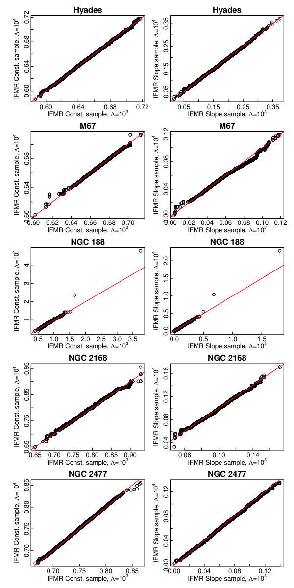
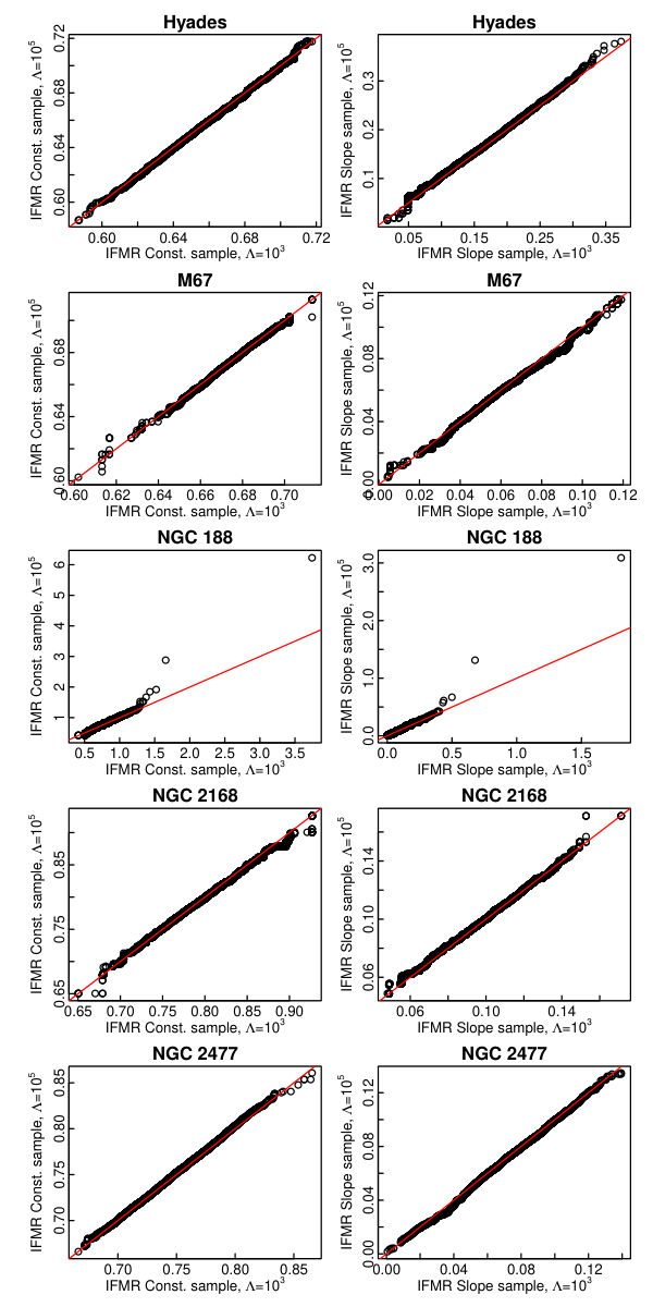
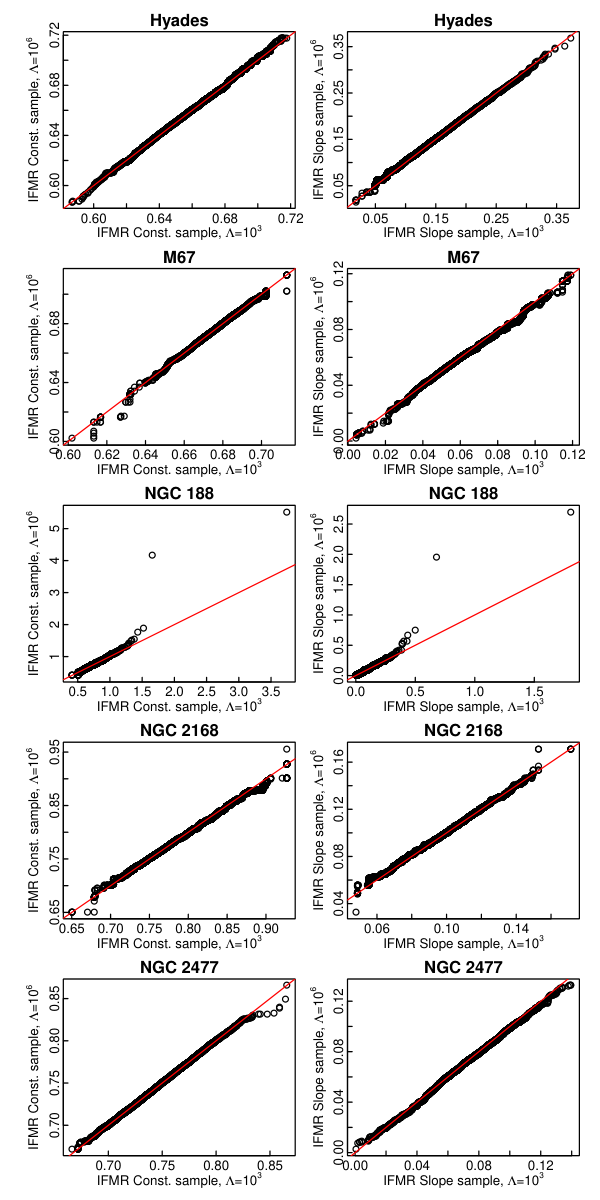
Fig.s 9–11 present the QQ plots of IFMR parameters from the hierarchical fits when takes different values. All points in these QQ plots lie close to the red line, meaning that MCMC draws of IFMR parameters are essentially the same. Though there are some small deviations from the red line, they are mainly caused by Monte Carlo errors. So we conclude that the hierarchical result is not sensitive to the choice of value of provided that .
5.2 Sensitivity to Membership of WDs in M67
Table 10 presents the hierarchical and case-by-case estimates of initial and final masses and membership probabilities for 35 WDs in M67, among which nine WDs have posterior membership probabilities less than and are classified as non-members or field stars. The other 26 WDs are inferred as members of M67. In this section we investigate whether the membership of these nine WDs affects the case-by-case posterior distribution of cluster M67.
In Section 4, when performing the case-by-case analysis on the cluster M67 with BASE-9, we set the prior membership probabilities of all WDs based on other research (Bellini et al., 2010a; Bellini et al., 2010b; Williams et al., 2013; Barnes et al., 2016, e.g.,). For clarity, we call this analysis the original fit. Then we fit M67 under two other circumstances: 1.) Case I: setting all WDs to have a 100% prior probability of being a member in M67, and 2.) Case II: assigning nine non-members as determined by the original fit (Table 10) to have prior membership probabilities equal to 0 and the apparent cluster members to have prior probabilities equal to 1. In other words, the first case forces all WDs in M67 to be cluster members whereas the second case removes nine apparent non-members and assumes that the other 26 as definitive cluster members.
Table 15 presents the point estimates of M67 parameters under three settings. The last two columns present the IFMR constant and slope, respectively. The case-by-case estimates of the IFMR slope vary under different settings. In Case I, when all WDs are forced to be M67 members, the IFMR slope is the steepest, while in the original fit, the IFMR is the shallowest. The estimates of other parameters are similar under the settings except the age. The estimate of age from the original fit is consistent to that from the Case II, while the age estimate from Case I is younger than the others. The age estimates from the original fit and Case I are close to the results obtained through other approaches (Bellini et al., 2010b; Williams et al., 2013).
| Settings | Age (Gyr) | [Fe/H]1 | Abs.1 | IFMR Constant | IFMR Slope | |
|---|---|---|---|---|---|---|
| Original | ||||||
| Case I | ||||||
| Case II | ||||||
| 1: The standard errors for metallicity and absorption under these fits | ||||||
| are all 0.01. | ||||||
Fig. 12 presents the CMD plots for these three fits. The black lines are from the fitted model under the original fit, and the red and blue lines are from models under Case I and II, respectively. From this plot, both fits from Case I (red line) and II (blue line) miss the main sequence turnoff stars, sub-giant branch and base of the red giant branch. By contrast, the model under the original fit (black line) matches both parts of the cluster well. We conclude that the original fit, where BASE-9 was able to assign its own cluster membership probabilities, is more reliable than the other fits. In summary, the membership of these WDs affect the posterior distribution of cluster parameters, yet our further analysis supports the original fit because it best matches the photometric data among those three fits.
5.3 Sensitivity to WD-WD Binaries
Our BASE-9 model does not include WD-WD binaries. While it will likely be preferable to do so eventually, current studies of cluster WDs are inadequate to determine the fraction of double degenerates in clusters and even further from determining which cluster WDs are unresolved binaries. The possible exceptions to this are the Hyades WDs, which are nearby, relatively bright, and well-studied. Among the 7 Hyades in our study, it is likely that all are single WDs. Theoretical studies (Hurley et al., 2005, e.g.,) indicate that the number of unresolved WD-WD binaries is probably % of a cluster’s WD population. Thus of the M67 WDs and each for NGC 188, NGC 2168, and NGC 2477 may be unresolved double degenerates. The WD regions of the CMDs for all of these clusters are consistent with this possibility. Fortunately, BASE-9 is robust against a small fraction of WDs having a large effect on the IFMR fit because (a) the double degenerate fraction is likely to be small and (b) objects that fall overly far from the best fit isochrones are fit as non-members and therefore do not contribute to the cluster solution (age, WD mass, IFMR parameters).
6 Conclusions and Discussions
We proposed a Bayesian hierarchical model for the IFMR parameters that simultaneously analyses data from multiple clusters in a single overall model and produces more precise estimates of the IFMR parameters. Also, we develop an efficient two-stage algorithm that takes advantage of existing software for cluster-specific analysis to obtain the fit under the hierarchical model. We combine data from five open clusters in the Bayesian hierarchical model and find that it can correct an error in the estimates of IFMR parameters for the cluster NGC 188 and produce reasonable estimates of IFMR for NGC 188. Based on our hierarchical analysis, we estimate the linear IFMR averaged across clusters to be
with .
This paper focus on the use of statistical techniques to the IFMR project, and the detailed results are preliminary. In particular, the astronomical results in this paper are not definitive and they depend upon the models inside the black-box code (in our case, the BASE-9) and other assumptions. Specifically, we assumed that the IFMR parameters from different clusters follow a bivariate normal distribution. However, this assumption might be too idealised. Bayesian hierarchical models always require a population distribution on all objects and the shape of the distribution of IFMR parameters across all clusters is not available. We therefore use the bivariate normal distribution as a starting point. If a case can be made for a different distribution, the statistical algorithm developed in this chapter will work as long as the case-by-case results are valid. Studies have indicated that metallicity may affect the IFMR (Kalirai et al., 2005; Catalan et al., 2008; Meng et al., 2008; Zhao et al., 2012, See, e.g.,). We showed how the Bayesian hierarchical model in Eq. (6) can be readily extended to investigate the effect of metallicity. In addition, even though our research is based on the BASE-9 package, our statistical techniques can be employed with other black-box packages as long as they produce MCMC samples in their case-by-case fits. Different underlying stellar evolution models will affect the results of case-by-case fits, hence they will most likely impact the resulting hierarchical fit. Our statistical approach and computational algorithm are independent of these inputs and can be broadly applied.
Acknowledgements
We thank the Imperial College High Performance Computing support team for their kind help, which greatly accelerated the simulation study in this project. Shijing Si thanks the Department of Mathematics in Imperial College London for a Roth studentship, which supported his research. David van Dyk acknowledges support from a Marie-Skodowska-Curie RISE Grant (H2020-MSCA-RISE-2015-691164) provided by the European Commission. Ted von Hippel acknowledges support from the National Science Foundation under Award AST-1715718. The authors gratefully thank the Referee and editors for the constructive comments and recommendations which definitely helped to improve the readability and quality of the paper. All the comments are addressed accordingly and have been incorporated to the revised manuscript.
References
- Andrews et al. (2015) Andrews J. J., Agüeros M. A., Gianninas A., Kilic M., Dhital S., Anderson S. F., 2015, Astrophysical Journal, 815, 63
- Babusiaux et al. (2018) Babusiaux C., et al., 2018, Astronomy & Astrophysics
- Barnes et al. (2016) Barnes S. A., Weingrill J., Fritzewski D., Strassmeier K. G., Platais I., 2016, Astrophysical Journal, 823, 16
- Bellini et al. (2010a) Bellini A., Bedin L., Pichardo B., Moreno E., Allen C., Piotto G., Anderson J., 2010a, Astronomy and Astrophysics, 513, 51
- Bellini et al. (2010b) Bellini A., et al., 2010b, Astronomy and Astrophysics, 513, 50
- Bergeron et al. (1995) Bergeron P., Wesemael F., Beauchamp A., 1995, Publications of the Astronomical Society of the Pacific, 107, 1047
- Browne & Goldstein (2002) Browne W., Goldstein H., 2002, Technical report, An Introduction to Bayesian Multilevel Hierarchical Modelling using MLwiN. Institute of Education, London
- Browne et al. (2006) Browne W. J., Draper D., et al., 2006, Bayesian analysis, 1, 473
- Catalan et al. (2008) Catalan S., Isern J., García-Berro E., Ribas I., 2008, Monthly Notices of the Royal Astronomical Society, 387, 1693
- Choi et al. (2016) Choi J., Dotter A., Conroy C., Cantiello M., Paxton B., Johnson B. D., 2016, Astrophysical Journal, 823, 102
- Clopper & Pearson (1934) Clopper C. J., Pearson E. S., 1934, Biometrika, 26, 404
- Cummings et al. (2016) Cummings J. D., Kalirai J. S., Tremblay P.-E., Ramirez-Ruiz E., 2016, Astrophysical Journal, 818, 84
- DeGennaro (2009) DeGennaro S., 2009, PhD thesis, The University of Texas at Ausin
- DeGennaro et al. (2009) DeGennaro S., von Hippel T., Jefferys W. H., Stein N., van Dyk D., Jeffery E., 2009, Astrophysical Journal, 696, 12
- Dotter et al. (2008) Dotter A., Chaboyer B., Jevremović D., Kostov V., Baron E., Ferguson J. W., 2008, Astrophysical Journal Supplement Series, 178, 89
- Gelman (2006) Gelman A., 2006, Technometrics, 48, 241
- Gelman et al. (2013) Gelman A., Carlin J. B., Stern H. S., Rubin D. B., 2013, Bayesian data analysis. Chapman & Hall/CRC Texts in Statistical Science Vol. 3, Taylor & Francis
- Girardi et al. (2000) Girardi L., Bressan A., Bertelli G., Chiosi C., 2000, Astronomy and Astrophysics Supplement Series, 141, 371
- Huang & Wand (2013) Huang A., Wand M. P., 2013, Bayesian Analysis, 8, 439
- Hurley et al. (2005) Hurley J. R., Pols O. R., Aarseth S. J., Tout C. A., 2005, Monthly Notices of the Royal Astronomical Society, 363, 293
- Jeffery et al. (2011) Jeffery E. J., von Hippel T., DeGennaro S., van Dyk D. A., Stein N., Jefferys W. H., 2011, Astrophysical Journal, 730, 35
- Jiao et al. (2016) Jiao X., van Dyk D. A., Trotta R., Shariff H., 2016, The Efficiency of Next-Generation Gibbs-Type Samplers: An Illustration Using a Hierarchical Model in Cosmology. Springer
- Kalirai et al. (2005) Kalirai J. S., Richer H. B., Reitzel D., Hansen B. M., Rich R. M., Fahlman G. G., Gibson B. K., von Hippel T., 2005, Astrophysical Journal, 618, L123
- Kalirai et al. (2008) Kalirai J. S., Hansen B. M., Kelson D. D., Reitzel D. B., Rich R. M., Richer H. B., 2008, Astrophysical Journal, 676, 594
- Kalirai et al. (2014) Kalirai J. S., Marigo P., Tremblay P.-E., 2014, Astrophysical Journal, 782, 17
- Lindegren et al. (2018) Lindegren L., Hernandez J., Bombrun A., Klioner S., et al., 2018, Astronomy & Astrophysics,
- Mandel et al. (2017) Mandel K. S., Scolnic D. M., Shariff H., Foley R. J., Kirshner R. P., 2017, Astrophysical Journal, 842, 93
- Marigo, P. & Girardi, L. (2007) Marigo, P. Girardi, L. 2007, Astronomy & Astrophysics, 469, 239
- Meibom et al. (2009) Meibom S., et al., 2009, Astronomical Journal, 137, 5086
- Meng et al. (2008) Meng X., Chen X., Han Z., 2008, Astronomy and Astrophysics, 487, 625
- Miller & Scalo (1979) Miller G. E., Scalo J. M., 1979, Astrophysical Journal Supplement Series, 41, 513
- Montgomery et al. (1999) Montgomery M., Klumpe E., Winget D., Wood M., 1999, Astrophysical Journal, 525, 482
- Morris & Lysy (2012) Morris C. N., Lysy M., 2012, Statistical Science, 27, 115
- Perryman et al. (1998) Perryman M. A. C., et al., 1998, Astronomy and Astrophysics, 331, 81
- R Core Team (2017) R Core Team 2017, R: A Language and Environment for Statistical Computing. R Foundation for Statistical Computing, Vienna, Austria, https://www.R-project.org/
- Salaris et al. (2009) Salaris M., Serenelli A., Weiss A., Bertolami M. M., 2009, Astrophysical Journal, 692, 1013
- Shariff et al. (2016) Shariff H., Jiao X., Trotta R., van Dyk D. A., 2016, Astrophysical Journal, 827, 1
- Si & van Dyk (2018) Si S., van Dyk D. A., 2018, Simple Two-Stage Algorithms for Fitting Hierarchies of Complex Models, In preparation
- Si et al. (2017a) Si S., van Dyk D. A., von Hippel T., Robinson E., Webster A., Stenning D., 2017a, Monthly Notices of the Royal Astronomical Society, 468, 4374
- Si et al. (2017b) Si S., van Dyk D. A., von Hippel T., 2017b, in Tremblay P.-E., Gaensicke B., Marsh T., eds, Astronomical Society of the Pacific Conference Series Vol. 509, 20th European White Dwarf Workshop. pp 69–72
- Stein et al. (2013) Stein N. M., van Dyk D. A., von Hippel T., DeGennaro S., Jeffery E. J., Jefferys W. H., 2013, Statistical Analysis and Data Mining: The ASA Data Science Journal, 6, 34
- Stenning et al. (2016) Stenning D., Wagner-Kaiser R., Robinson E., Van Dyk D., Von Hippel T., Sarajedini A., Stein N., 2016, Astrophysical Journal, 826, 41
- Sung & Bessell (1999) Sung H., Bessell M., 1999, Monthly Notices of the Royal Astronomical Society, 306, 361
- Taylor (2006) Taylor B., 2006, Astronomical Journal, 133, 370
- VandenBerg & Stetson (2004) VandenBerg D. A., Stetson P., 2004, Publications of the Astronomical Society of the Pacific, 116, 997
- Williams et al. (2004) Williams K. A., Bolte M., Koester D., 2004, Astrophysical Journal Letters, 615, L49
- Williams et al. (2009) Williams K. A., Bolte M., Koester D., 2009, Astrophysical Journal, 693, 355
- Williams et al. (2013) Williams K. A., Howell S. B., Liebert J., Smith P. S., Bellini A., Rubin K. H., Bolte M., 2013, Astronomical Journal, 145, 129
- Zhao et al. (2012) Zhao J. K., Oswalt T. D., Willson L. A., Wang Q., Zhao G., 2012, Astrophysical Journal, 746, 144
- de Bruijne, J. H. J. et al. (2001) de Bruijne, J. H. J. Hoogerwerf, R. de Zeeuw, P. T. 2001, Astronomy & Astrophysics, 367, 111
- van Dyk & Park (2008) van Dyk D. A., Park T., 2008, Journal of the American Statistical Association, 103, 790
- van Dyk et al. (2009) van Dyk D. A., Degennaro S., Stein N., Jefferys W. H., von Hippel T., 2009, Annals of Applied Statistics, 3, 117
- von Hippel & Sarajedini (1998) von Hippel T., Sarajedini A., 1998, Astronomical Journal, 116, 1789
- von Hippel et al. (2006) von Hippel T., Jefferys W. H., Scott J., Stein N., Winget D., DeGennaro S., Dam A., Jeffery E., 2006, Astrophysical Journal, 645, 1436
- von Hippel et al. (2014) von Hippel T., et al., 2014, arXiv preprint arXiv:1411.3786
Appendix A Computational Algorithm
The joint posterior distribution in Eq. 7 is high-dimensional, with parameters. In this appendix, we show how to take advantage of the cluster-specific fittings in BASE-9 via a two-stage (TS) algorithm to fit the hierarchical model.
To simplify the description of the TS algorithm, we introduce for . We use .
- Step 0a:
-
For each star cluster run BASE-9 to obtain a Monte Carlo sample of via the cluster-specific analysis. Thin each chain to obtain an essentially independent Monte Carlo sample and label it .
- Step 0b:
-
In the following, we denote the TS samples with the tilde notation. Simulate random integers between and , denote them , and initialise the parameters and for .
- Step 0c:
- Step 0d:
-
Given , we simulate from their conditional posterior distributions,
for .
For , run Step 1 and Step 2 iteratively. - Step 1:
-
Randomly generate integers between and , and denote them . For each , set and as the new proposal and set with probability . Otherwise, set .
- Step 2:
-
Given and , update via
with .
Given , simulate via
Appendix B Photometry Data for WDs in Five Star Clusters
Here are the photometry data for the WDs in these five star clusters in Section 4.
| Cluster | WD | |||
|---|---|---|---|---|
| Hyades | HZ14 | |||
| VR16 | ||||
| HZ7 | ||||
| VR7 | ||||
| HZ4 | ||||
| LB227 | ||||
| References: DeGennaro et al. (2009); Stein et al. (2013) | ||||
| Cluster | WD | ||
|---|---|---|---|
| M67 | WD 1 | ||
| WD 2 | |||
| WD 3 | |||
| WD 4 | |||
| WD 5 | |||
| WD 6 | |||
| WD 7 | |||
| WD 8 | |||
| WD 9 | |||
| WD 10 | |||
| WD 11 | |||
| WD 12 | |||
| WD 13 | |||
| WD 14 | |||
| WD 15 | |||
| WD 16 | |||
| WD 17 | |||
| WD 18 | |||
| WD 19 | |||
| WD 20 | |||
| WD 21 | |||
| WD 22 | |||
| WD 23 | |||
| WD 24 | |||
| WD 25 | |||
| WD 26 | |||
| WD 27 | |||
| WD 28 | |||
| WD 29 | |||
| WD 30 | |||
| WD 31 | |||
| WD 32 | |||
| WD 33 | |||
| WD 34 | |||
| WD 35 | |||
| References: Bellini et al. (2010a); Bellini et al. (2010b) | |||
| Cluster | WD | ||||
|---|---|---|---|---|---|
| NGC188 | WD 1 | ||||
| WD 2 | |||||
| WD 3 | |||||
| WD 4 | |||||
| WD 5 | |||||
| WD 6 | |||||
| WD 7 | |||||
| WD 8 | |||||
| WD 9 | |||||
| NGC2168 | WD 1 | ||||
| WD 2 | |||||
| WD 3 | |||||
| WD 4 | |||||
| WD 5 | |||||
| WD 6 | |||||
| WD 7 | |||||
| WD 8 | |||||
| WD 9 | |||||
| WD 10 | |||||
| WD 11 | |||||
| WD 12 | |||||
| WD 13 | |||||
| NGC2477 | WD 1 | ||||
| WD 2 | |||||
| WD 3 | |||||
| WD 4 | |||||
| WD 5 | |||||
| WD 6 | |||||
| WD 7 | |||||
| References for NGC188: von Hippel & Sarajedini (1998); Meibom et al. (2009) | |||||
| References for NGC2168: Sung & Bessell (1999); Williams et al. (2004) | |||||
| References for NGC2477: Jeffery et al. (2011); Stein et al. (2013) | |||||