跳到论文正文
W Papers独立论文阅读器 arXiv:1806.06732 论文正文 计算阅读时间 · 0%
引用这篇论文根据当前论文元数据生成,正式投稿前建议核对。


License: arXiv.org perpetual non-exclusive license
arXiv:1806.06732v2 [math.NA] 28 Sep 2019

A damped second order flow \shortauthorlistG. Baravdish et al.

Damped second order flow applied to image denoising

\nameG. Baravdish and O. Svensson \nameM. Gulliksson Address: Department of Science and Technology, Linköping University, 58183 Linköping, Sweden Address: School of Science and Technology, Örebro University, 70182 Örebro, Sweden    \nameY. Zhang∗ Email: $ˆ*$Corresponding author: ye.zhang@oru.se Address: Shenzhen MSU-BIT University, 518172 Shenzhen, China, and School of Mathematics and Statistics, Beijing Institude of Technology, 100081 Beijing, China
Abstract

In this paper, we introduce a new image denoising model: the damped flow (DF), which is a second order nonlinear evolution equation associated with a class of energy functionals of an image. The existence, uniqueness, and regularization property of DF are proven. For the numerical implementation, based on the Störmer-Verlet method, a discrete damped flow, SV-DDF, is developed. The convergence of SV-DDF is studied as well. Several numerical experiments, as well as a comparison with other methods, are provided to demonstrate the efficiency of SV-DDF. nonlinear flow; image denoising; pp-parabolic; pp-Laplace; inverse problems; regularization; damped Hamiltonian system; symplectic method; Störmer-Verlet.
2000 Math Subject Classification: 35A01, 35A02, 65P10, 65M12, 65M32

1 Introduction.

Digital images play a significant role in many fields in science, industry, and daily life, such as computer tomography, magnetic resonance imaging, geographical information systems, astronomy, satellite television, etc. Data sets collected by image sensors are always contaminated by noise. Instrument precision, the absence of some acquisition channels, and interfering natural phenomena can all degrade the data information. Moreover, noise can be introduced by transmission errors, compression and artificial editing. Therefore, it is necessary to apply a denoising technique on the original noisy image before it is analyzed.

Over the last few decades, scientists have developed numerous techniques to achieve adaptive imaging denoising, such as wavelets ([Donoho & Johnstone(1995)Donoho & Johnstone]), stochastic approaches ([Preusser et al.(2008)Preusser, Scharr, Krajsek, & Kirby]), and formulations based on partial differential equations (PDEs) ([Alvarez et al.(1993)Alvarez, Guichard, Lions, & Morel, Weickert(1998)Weickert]). We refer to ([Gonzalez & Woods(2007)Gonzalez & Woods, Scherzer et al.(2009)Scherzer, Grasmair, Grossauer, Haltmeier, & Lenzen]) for a review on various denoising methods.

An essential challenge for imaging denoising is to remove noise as much as possible without eliminating the most representative characteristics of the image, such as edges, corners and other sharp structures. Traditional denoising methods are given some information about the noise, but the problem of blind image denoising involves computing the denoised image from the noisy one without any knowledge of the noise. The energy functional approach has in recent years been very successful in blind image denoising, most often taking the form

ℰ⁡(u)=12​∫Ω(u−u0)2​𝑑x+α​∫ΩΦ⁡(|∇u|)​𝑑x,\mathcal{E}(u)=\frac{1}{2}\int_{\Omega}(u-u_{0})^{2}dx+\alpha\int_{\Omega}\Phi(|\nabla u|)dx, (1)

where u0​(x)u_{0}(x) is the observed (noisy) image, and Ω⊂𝐑N\Omega\subset\mathbf{R}^{N} (N=2,3N=2,3) is a bounded domain with almost everywhere C2C^{2} smooth boundary ∂Ω\partial\Omega. The first term in (1) is a fidelity term, the second term is a regularization term, and α>0\alpha>0 is the regularization parameter. The regularization term Φ⁡(|∇u|)\Phi(|\nabla u|) is usually assumed to be strictly convex. A well-studied case of ℰ⁡(u)\mathcal{E}(u) is when the regularization term is the pp-Dirichlet energy, i.e., Φ⁡(|∇u|)=1p​|∇u|p,p≥1\Phi(|\nabla u|)=\frac{1}{p}|\nabla u|^{p},p\geq 1. The cases p=1p=1 and p=2p=2 correspond to the Total Variation (TV) principle ([Rudin et al.(1992)Rudin, Osher, & Fatemi]) and the first-order Tikhonov’s regularization, respectively. The general cases for p>1p>1 and p=p⁡(x)p=p(x) have been studied in, e.g., [Baravdish et al.(2015)Baravdish, Svensson, & Åström, Kuijper(2009)Kuijper]. Nowadays, there are many relevant extensions of the TV model, e.g., [Bollt et al.(2009)Bollt, Chartrand, Esedolu, Schultz, & Vixie, Bredies et al.(2010)Bredies, Kunisch, & Pock, Chen et al.(2006)Chen, Levine, & Rao]. The extension of TV to variational tensor-based formulations was investigated in [Grasmair & Lenzen(2010)Grasmair & Lenzen]. Other relevant extensions of the energy functional can be found in [Åström et al.(2017)Åström, Felsberg, & Baravdish].

The Euler-Lagrange equation ∂ℰ/∂u=0\partial\mathcal{E}/\partial u=0 associated with the functional ℰ⁡(u)\mathcal{E}(u) is given by

u−u0−α⋅div(Φ′​(|∇u|)|∇u|∇u)=0 in Ω,∂nu=0 on ∂Ω,u-u_{0}-\alpha\cdot\textmd{div}\left(\frac{\Phi^{\prime}(|\nabla u|)}{|\nabla u|}\nabla u\right)=0\textmd{~in~}\ \Omega,\quad\partial_{n}u=0\textmd{~on~}\ \partial\Omega, (2)

where nn is the outward unit normal to the boundary ∂Ω\partial\Omega. For the pp-Dirichlet energy, let α→0\alpha\to 0, and we obtain the first order flow

ut−Δp​u=0​ in ​(0,T)×Ω,u⁡(x,0)=u0​(x)​ in ​Ω,u_{t}-\Delta_{p}u=0\textmd{~in~}\ (0,T)\times\Omega,\quad u(x,0)=u_{0}(x)\textmd{~in~}\ \Omega, (3)

where the pp-Laplace operator is defined by Δpu=div(|∇u|p−2∇u)\Delta_{p}u=\textmd{div}\left(|\nabla u|^{p-2}\nabla u\right). The pp-parabolic equation in (3) has been studied intensively in [DiBenedetto(1993)DiBenedetto, Ladyzhenskaja et al.(1988)Ladyzhenskaja, Solonnikov, & Uraltseva, Lieberman(1996)Lieberman, Roubíček(2013)Roubíček, Wu et al.(2001)Wu, Yin, Li, & Zhao], and references therein. The edge detection property of (3) has been analyzed in [Perona & Malik(1990)Perona & Malik], where instead of the pp-Laplace operator, they studied a more general diffusion term div(g(|∇u|)∇u)\textmd{div}\left(g(|\nabla u|)\nabla u\right). The main advantage of (3) is the so-called conditional smoothing capability: For large ∇u\nabla u, the diffusion will be low, and therefore the exact localization of the edges will be kept. While ∇u​(x)\nabla u(x) is small, the diffusion will tend to smooth around xx. However, in the case of small noise of uu with large oscillations of the gradient ∇u\nabla u, the conditional smoothing introduced by (3) will keep all noise edges. To avoid the above mentioned difficulty, the authors in [Alvarez et al.(1992)Alvarez, Lions, & Morel] proposed a selective smoothing model

ut−div(g(|∇Gσ⋆u|)∇u)=0,u_{t}-\textmd{div}\left(g(|\nabla G_{\sigma}\star u|)\nabla u\right)=0, (4)

where gg is a smooth nonnegtive nonincreasing function with g⁡(0)=1g(0)=1 and limr→+∞g⁡(r)=0\lim_{r\to+\infty}g(r)=0. In (4), Gσ​(x)G_{\sigma}(x), σ>0\sigma>0, is the Gaussian kernel Gσ​(x)=1(2​π​σ)N/2​e−|x|22​σG_{\sigma}(x)=\frac{1}{(2\pi\sigma)^{N/2}}e^{-\frac{|x|^{2}}{2\sigma}}, |∇Gσ⋆u|2=∑j=1N(∂Gσ∂xj⋆u)2|\nabla G_{\sigma}\star u|^{2}=\sum_{j=1}^{N}\left(\frac{\partial G_{\sigma}}{\partial x_{j}}\star u\right)^{2}, and ⋆\star denote the cross-correlation, namely (f⋆g)​(x)=∫𝐑Nf¯​(y)​g​(x+y)​𝑑y(f\star g)(x)=\int_{\mathbf{R}^{N}}\bar{f}(y)g(x+y)dy, f¯\bar{f} is the complex conjugate of ff.

On the other hand, for a better edge preservation, the authors in [Ratner & Zeevi(2011)Ratner & Zeevi, Ratner & Zeevi(2013)Ratner & Zeevi] introduced a Telegraph-Diffusion (TeD) model, which is described by a second order (in time) hyperbolic equation

ut​t+ηut−div(k∇u)=0,u(x,0)=u0(x),ut(x,0)=0 in Ω,u_{tt}+\eta u_{t}-\textmd{div}\left(k\nabla u\right)=0,\quad u(x,0)=u_{0}(x),u_{t}(x,0)=0\textmd{~in~}\ \Omega, (5)

where η\eta and kk denote the damping and elasticity coefficients, respectively. It has been shown that the model (5) enables better preservation of edges in image denoising by offering an adaptive lowpass filter, and offering slower error propagation across edges.

Inspired by imaging denosing models (4) and (5), in this paper, we will study the following second order flow

{ut​t+ηut−div((ε+|∇Gσ⋆u|2)p−22∇u)=0in​(0,T)×Ω,u​(x,0)=u0​(x)in​Ω,ut​(x,0)=0in​Ω,∂nu=0on​∂Ω.\left\{\begin{array}[]{rl}u_{tt}+\eta u_{t}-\textmd{div}\left((\varepsilon+|\nabla G_{\sigma}\star u|^{2})^{\frac{p-2}{2}}\nabla u\right)=0&\textmd{in}\ (0,T)\times\Omega,\\ u(x,0)=u_{0}(x)&\textmd{in}\ \Omega,\\ u_{t}(x,0)=0&\textmd{in}\ \Omega,\\ \partial_{n}u=0&\textmd{on}\ \partial\Omega.\end{array}\right. (6)

where the damping parameter η>0\eta>0 is a given model parameter, and σ,ε>0\sigma,\varepsilon>0 are two anther given small numbers, which are used to avoid the singularity of model (6).

The model (6) can be viewed as a regularized version of the telegraphers’ equation with the pp-Laplace operator, i.e. ut​t+η​ut−Δp​u=0u_{tt}+\eta u_{t}-\Delta_{p}u=0. Denote by V⁡(u)=∫Ω1p​|∇u|p​𝑑xV(u)=\int_{\Omega}\frac{1}{p}|\nabla u|^{p}dx the pp-Dirichlet integral. Then, the first order flow in (3), i.e. ut+∂uV⁡(u)=0u_{t}+\partial_{u}V(u)=0, can be considered a classical steepest descent flow for solving the optimization problem minu⁡V⁡(u)\min_{u}V(u). In the last two decades, there has been increasing evidence found showing that second order flows also enjoy remarkable optimization properties. Among these, a particularly important dynamical system – ut​t+η​ut+∂uV⁡(u)=0u_{tt}+\eta u_{t}+\partial_{u}V(u)=0 – is called the Heavy Ball with Friction system (HBF) ([Attouch et al.(2000)Attouch, Goudou, & Redont]) because of its mechanical interpretation. This system is an asymptotic approximation of the equation describing the motion of a material point with positive mass, subjected to stay on the graph of V⁡(u)V(u), and which moves under the action of the gravity force, the reaction force, and the friction force (η>0\eta>0 is the friction parameter). The introduction of the term u¨​(t)\ddot{u}(t) in the dynamical system permits it to overcome some of the drawbacks of the steepest descent method. By contrast with steepest descent methods, the HBF system is not a descent method. It is the global energy (kinetic plus potential) which decreases. The optimization properties for the HBF system have been studied in detail in [Alvarez(2000)Alvarez, Alvarez et al.(2002)Alvarez, Attouch, Bolte, & Redont, Attouch et al.(2000)Attouch, Goudou, & Redont], and references therein. Numerical algorithms based on the HBF system of solving some special problems, e.g. large systems of linear equations, eigenvalue problems, nonlinear Schrödinger problems, inverse source problems, general ill posed problems, etc., can be found in [Edvardsson et al.(2012)Edvardsson, Gulliksson, & Persson, Edvardsson et al.(2015)Edvardsson, Neuman, Edström, & Olin, Sandin et al.(2016)Sandin, Ögren, & Gulliksson, Zhang et al.(2018)Zhang, Gong, Cheng, & Gulliksson, Zhang & Hofmann(2018)Zhang & Hofmann, Gong et al.(2019)Rong, Hofmann, & Zhang], where we can see that a second order damped system solved by a symplectic solver is far more efficient than numerically solving a first order system. In this study, we focus on the regularity of the specific system (6) and its denoising capability.

The remainder of the paper is structured as follows. In Section 2, we study the existence and uniqueness of PDE (6). Section 3 briefly discusses the regularization property of the dynamical solution with (6). Based on the Störmer-Verlet method, a discrete damped flow, termed by SV-DDF, is proposed in Section 4, where the convergence property of SV-DDF is studied. Section 5 presents an algorithm for image denoising. Several numerical examples are presented in Section 6 to demonstrate the feasibility and efficiency of the proposed method. A comparison with other methods is provided as well. Finally, concluding remarks are given in Section 7.

2 Well-posedness of the model: Existence and uniquness results.

We start with a brief description of the mathematical principles and some of the definitions used in this work. We denote by Hk​(Ω)H^{k}(\Omega), where kk is a positive integer, and the set of all functions uu defined in Ω\Omega is such that its distributional derivatives Ds=∂su/∂xsD^{s}=\partial^{s}u/\partial x^{s} of order |s|=∑i=1ksi≤k|s|=\sum_{i=1}^{k}s_{i}\leq k all belong to L2​(Ω)L^{2}(\Omega). Furthermore, Hk​(Ω)H^{k}(\Omega) is a Hilbert space with the norm ‖u‖Hk​(Ω)=(∑s≤k∫Ω|Ds​u|2​𝑑x)1/2.\|u\|_{H^{k}(\Omega)}=\left(\sum_{s\leq k}\int_{\Omega}|D^{s}u|^{2}\,dx\right)^{1/2}. The space Lp​(0,T,Hk​(Ω))L^{p}(0,T;H^{k}(\Omega)) consists of all functions uu such that for almost every t∈(0,T)t\in(0,T), the element u⁡(t)u(t) belongs to Hk​(Ω)H^{k}(\Omega). Hence, Lp​(0,T,Hk​(Ω))L^{p}(0,T;H^{k}(\Omega)) is a normed space with the norm ‖u‖Lp​(0,T,Hk​(Ω))=(∫0T‖u‖Hk​(Ω)p​𝑑t)1/p,\|u\|_{L^{p}(0,T;H^{k}(\Omega))}=\left(\int_{0}^{T}\|u\|_{H^{k}(\Omega)}^{p}\,dt\right)^{1/p}, where p>1p>1. We also denote by L∞​(0,T,X)L^{\infty}(0,T;X) the set of all functions uu such that for almost every t∈(0,T)t\in(0,T) the element u⁡(t)u(t) belongs to XX. L∞​(0,T,X)L^{\infty}(0,T;X) is a normed space with the norm ‖u‖L∞​(0,T,X)=inf​{C;‖u⁡(t)‖X≤C, a.e. on ​(0,T)}.\|u\|_{L^{\infty}(0,T;X)}=\textmd{inf}\{C;\ \|u(t)\|_{X}\leq C,\mbox{ a.e. on }(0,T)\}. We denote by H1​(Ω)∗H^{1}(\Omega)^{*} the dual space of H1​(Ω)H^{1}(\Omega). In the following, let CiC_{i} denote a constant with a different value at a different place. It does not depend on the estimated quality. Moreover, to simplify the notation, we put

aε(∇Gσ⋆u)=(ε+|∇Gσ⋆u|2)p−22,p∈[1,2],a^{\varepsilon}(\nabla G_{\sigma}\star u)=(\varepsilon+|\nabla G_{\sigma}\star u|^{2})^{\frac{p-2}{2}},\quad p\in[1,2], (7)

and sometimes let ut​(t)=u′​(t)u_{t}(t)=u^{\prime}(t).

Next, we introduce the solution space 𝒰\mathcal{U} for the problem (6).

Definition 2.1.

We say that an element uu belongs to the solution space 𝒰\mathcal{U} for the problem (6) if u∈L∞​(0,T,H1​(Ω))u\in L^{\infty}(0,T;H^{1}(\Omega)), and its derivatives u′u^{\prime} and u′′u^{\prime\prime} with respect to tt in the sense of distributions to the spaces L∞​(0,T,L2​(Ω))L^{\infty}(0,T;L^{2}(\Omega)) and L∞​(0,T,H1​(Ω)∗)L^{\infty}(0,T;H^{1}(\Omega)^{*}) respectively.

It is easily seen that 𝒰\mathcal{U} is a Banach space equipped with the norm

‖u‖𝒰=‖u‖L∞​(0,T,H1​(Ω))+‖u′‖L∞​(0,T,L2​(Ω))+‖u′′‖L∞​(0,T,H1​(Ω)∗).\|u\|_{\mathcal{U}}=\|u\|_{L^{\infty}(0,T;H^{1}(\Omega))}+\|u^{\prime}\|_{L^{\infty}(0,T;L^{2}(\Omega))}+\|u^{\prime\prime}\|_{L^{\infty}(0,T;H^{1}(\Omega)^{*})}.

The solutions for the problem (6) are considered in the weak sense, as follows.

Definition 2.2.

A function uu is called a weak solution of the problem (6) if u∈𝒰u\in\mathcal{U} and satisfies (6) for almost every t∈(0,+∞)t\in(0,+\infty) with derivatives of uu in the sense of distributions.

We will show the existence of weak solutions for problem (6) by using the Schauder fixed point theorem; see [Cao et al.(2010)Cao, Yin, Liu, & Li, Catté et al.(1992)Catté, Lions, Morel, & Coll]. In the sequel, we need the following results for the corresponding linear problem, [Evans(2010)Evans], namely,

{ut​t+ηut−div(b(x,t)∇u)=0in​(0,T)×Ω,u​(x,0)=u0​(x)in​Ω,ut​(x,0)=0in​Ω∂nu=0on​∂Ω.,\left\{\begin{array}[]{rl}u_{tt}+\eta u_{t}-\textmd{div}(b(x,t)\nabla u)=0&\textmd{in}\ (0,T)\times\Omega,\\ u(x,0)=u_{0}(x)&\textmd{in}\ \Omega,\\ u_{t}(x,0)=0&\textmd{in}\ \Omega\\ \partial_{n}u=0&\textmd{on}\ \partial\Omega.\end{array}\right., (8)

where b⁡(x,t)b(x,t) is a given function such that b⁡(x,t)≥c>0b(x,t)\geq c>0 and cc is a constant.

Theorem 2.3.

Suppose that b⁡(x,t)b(x,t) is bounded, and let u0∈H1​(Ω)u_{0}\in H^{1}(\Omega). Then the problem in (8) has a unique solution u∈𝒰u\in{\mathcal{U}}. Moreover, if u0∈H2​(Ω)u_{0}\in H^{2}(\Omega), then it follows that ut∈L∞​(0,T,H1​(Ω))u_{t}\in L^{\infty}(0,T;H^{1}(\Omega)).

The linear problem (8) is by now well-studied and Theorem 2.3 can be proven by the Galerkin method, see [Evans(2010)Evans]. Before providing the main result, let us consider the following lemma.

Lemma 2.4.

Assume that for all x∈Ωx\in\Omega and a.e. t∈(0,T)t\in(0,T) there exists a positive constant CC depending on GσG_{\sigma} and Ω\Omega such that

||∇Gσ⋆v||L∞​(0,T,L∞​(Ω))≤C||u0||H1​(Ω),||∇Gσ⋆vt||L∞​(0,T,L∞​(Ω))≤C||u0||H1​(Ω),∀v∈𝒰.\displaystyle||\nabla G_{\sigma}\star v||_{L^{\infty}(0,T;L^{\infty}(\Omega))}\leq C||u_{0}||_{H^{1}(\Omega)},\quad||\nabla G_{\sigma}\star v_{t}||_{L^{\infty}(0,T;L^{\infty}(\Omega))}\leq C||u_{0}||_{H^{1}(\Omega)},\quad\forall v\in\mathcal{U}. (9)

Then, the following inequalities hold for p∈[1,2]p\in[1,2]

(ε+C2||u0||H1​(Ω)2)p−22≤aε(∇Gσ⋆v)≤εp−22,∀v∈𝒰\displaystyle(\varepsilon+C^{2}||u_{0}||^{2}_{H^{1}(\Omega)})^{\frac{p-2}{2}}\leq a^{\varepsilon}(\nabla G_{\sigma}\star v)\leq\varepsilon^{\frac{p-2}{2}},\quad\forall v\in\mathcal{U} (10)
|atε(∇Gσ⋆v)|≤(2−p)NC2εp−42||u0||H1​(Ω)2,∀v∈𝒰.\displaystyle|a_{t}^{\varepsilon}(\nabla G_{\sigma}\star v)|\leq(2-p)NC^{2}\varepsilon^{\frac{p-4}{2}}||u_{0}||^{2}_{H^{1}(\Omega)},\quad\forall v\in\mathcal{U}. (11)
Proof 2.5.

Inequalities (10) hold obviously by noting the definition of aεa^{\varepsilon} in (7) and the following inequalities

ε2−p2≤(ε+|∇Gσ⋆v|2)2−p2≤(ε+C2||u0||H1​(Ω)2)2−p2\displaystyle\varepsilon^{\frac{2-p}{2}}\leq(\varepsilon+|\nabla G_{\sigma}\star v|^{2})^{\frac{2-p}{2}}\leq(\varepsilon+C^{2}||u_{0}||^{2}_{H^{1}(\Omega)})^{\frac{2-p}{2}}

for p∈[1,2]p\in[1,2], and for all x∈Ωx\in\Omega and a.e. t∈(0,T)t\in(0,T).

Now, consider the inequality (11). Since

atε(∇Gσ⋆v)=p−22(ε+|∇Gσ⋆v|2)p−42∑j=1N2(∂Gσ∂xj⋆v)(∂Gσ∂xj⋆vt),\displaystyle a_{t}^{\varepsilon}(\nabla G_{\sigma}\star v)=\frac{p-2}{2}\left(\varepsilon+|\nabla G_{\sigma}\star v|^{2}\right)^{\frac{p-4}{2}}\sum_{j=1}^{N}2\left(\frac{\partial G_{\sigma}}{\partial x_{j}}\star v\right)\left(\frac{\partial G_{\sigma}}{\partial x_{j}}\star v_{t}\right),

we can deduce that

|atε(∇Gσ⋆v)|\displaystyle|a_{t}^{\varepsilon}(\nabla G_{\sigma}\star v)| =\displaystyle= (2−p)(ε+|∇Gσ⋆v|2)p−42⋅|∑j=1N(∂Gσ∂xj⋆v)(∂Gσ∂xj⋆vt)|\displaystyle(2-p)\left(\varepsilon+|\nabla G_{\sigma}\star v|^{2}\right)^{\frac{p-4}{2}}\cdot\left|\sum_{j=1}^{N}\left(\frac{\partial G_{\sigma}}{\partial x_{j}}\star v\right)\left(\frac{\partial G_{\sigma}}{\partial x_{j}}\star v_{t}\right)\right|
≤\displaystyle\leq (2−p)​εp−42⋅N⋅C2​‖u0‖H1​(Ω)2,\displaystyle(2-p)\varepsilon^{\frac{p-4}{2}}\cdot N\cdot C^{2}||u_{0}||^{2}_{H^{1}(\Omega)},

by noting the conditions of the lemma.

Now, we are in a position to show our main result.

Theorem 2.6.

Assume that p∈[1,2]p\in[1,2] and u0∈H2​(Ω)u_{0}\in H^{2}(\Omega). Then a unique weak solution to problem (6) exists if TT is sufficiently small with an upper bound depending on ‖u0‖H1​(Ω)||u_{0}||_{H^{1}(\Omega)}, GσG_{\sigma} and Ω\Omega.

Proof 2.7.

Existence. We use the Schauder fixed point theory, [Cao et al.(2010)Cao, Yin, Liu, & Li, Catté et al.(1992)Catté, Lions, Morel, & Coll], to prove the existence. Let v∈𝒰v\in\mathcal{U} be such that

‖v‖L∞​(0,T,L2​(Ω))+‖vt‖L∞​(0,T,L2​(Ω))≤C1||u0||H1​(Ω)||v||_{L^{\infty}(0,T;L^{2}(\Omega))}+||v_{t}||_{L^{\infty}(0,T;L^{2}(\Omega))}\leq C_{1}||u_{0}||_{H^{1}(\Omega)} (12)

where the positive constant C1C_{1} will be determined later. Then the elements ∇Gσ⋆v\nabla G_{\sigma}\star v and ∇Gσ⋆vt\nabla G_{\sigma}\star v_{t} belong to L∞​(0,T,C∞​(Ω))L^{\infty}(0,T;C^{\infty}(\Omega)), and for all x∈Ωx\in\Omega and a.e. t∈(0,T)t\in(0,T) a positive constant C2C_{2} depending on GσG_{\sigma} and Ω\Omega exists such that

||∇Gσ⋆v||L∞​(0,T,L∞​(Ω))≤C1C2||u0||H1​(Ω),||∇Gσ⋆vt||L∞​(0,T,L∞​(Ω))≤C1C2||u0||H1​(Ω).\displaystyle||\nabla G_{\sigma}\star v||_{L^{\infty}(0,T;L^{\infty}(\Omega))}\leq C_{1}C_{2}||u_{0}||_{H^{1}(\Omega)},\quad||\nabla G_{\sigma}\star v_{t}||_{L^{\infty}(0,T;L^{\infty}(\Omega))}\leq C_{1}C_{2}||u_{0}||_{H^{1}(\Omega)}.

By Lemma 2.4, for all x∈Ωx\in\Omega and a.e. tt in (0,T)(0,T), it follows that

(ε+C12C22||u0||H1​(Ω)2)p−22≤aε(∇Gσ⋆v)≤εp−22,\displaystyle(\varepsilon+C^{2}_{1}C^{2}_{2}||u_{0}||^{2}_{H^{1}(\Omega)})^{\frac{p-2}{2}}\leq a^{\varepsilon}(\nabla G_{\sigma}\star v)\leq\varepsilon^{\frac{p-2}{2}}, (13)
|atε(∇Gσ⋆v)|≤(2−p)N(C1C2)2εp−42||u0||H1​(Ω)2.\displaystyle|a_{t}^{\varepsilon}(\nabla G_{\sigma}\star v)|\leq(2-p)N(C_{1}C_{2})^{2}\varepsilon^{\frac{p-4}{2}}||u_{0}||^{2}_{H^{1}(\Omega)}. (14)

Let v∈𝒰v\in\mathcal{U} satisfy (12) and consider the problem PvP_{v}:

⟨ut​t,φ⟩H1​(Ω)∗×H1​(Ω)+∫Ω(ηutφ+aε(∇Gσ⋆v)∇u⋅∇φ)dx=0\langle u_{tt},\varphi\rangle_{H^{1}(\Omega)^{*}\times H^{1}(\Omega)}+\int_{\Omega}\left(\eta u_{t}\varphi+a^{\varepsilon}(\nabla G_{\sigma}\star v)\nabla u\cdot\nabla\varphi\right)\,dx=0 (15)

for every element φ∈H1​(Ω)\varphi\in H^{1}(\Omega), a.e. tt in (0,T)(0,T). The linear problem PvP_{v} in (15) is well-posed, [Evans(2010)Evans], and has a solution uvu_{v} which satisfies

‖uv‖H1​(Ω)≤C3​‖u0‖H1​(Ω),||u_{v}||_{H^{1}(\Omega)}\leq C_{3}||u_{0}||_{H^{1}(\Omega)}, (16)

where C3C_{3} is a positive constant, depending only on the domain Ω\Omega.

Now, let us consider two cases when φ=uv′\varphi=u_{v}^{\prime} and ϕ=uν\phi=u_{\nu}.

Case 1. If φ=uv′\varphi=u_{v}^{\prime}, we have

⟨uv′′,uv′⟩H1​(Ω)∗×H1​(Ω)+∫Ωη(uv′)2dx+∫Ωaε(∇Gσ⋆v)∇uv⋅∇uv′dx=0,\langle u_{v}^{\prime\prime},u_{v}^{\prime}\rangle_{H^{1}(\Omega)^{*}\times H^{1}(\Omega)}+\int_{\Omega}\eta(u_{v}^{\prime})^{2}\,dx+\int_{\Omega}a^{\varepsilon}(\nabla G_{\sigma}\star v)\nabla u_{v}\cdot\nabla u_{v}^{\prime}\,dx=0,

which gives

12dd​t⟨uv′,uv′⟩H1​(Ω)×H1​(Ω)+η∫Ω(uv′)2dx+∫Ωaε(∇Gσ⋆v)∇uv⋅∇uv′dx=0,\frac{1}{2}\frac{d}{dt}\langle u_{v}^{\prime},u_{v}^{\prime}\rangle_{H^{1}(\Omega)\times H^{1}(\Omega)}+\eta\int_{\Omega}(u_{v}^{\prime})^{2}\,dx+\int_{\Omega}a^{\varepsilon}(\nabla G_{\sigma}\star v)\nabla u_{v}\cdot\nabla u_{v}^{\prime}\,dx=0,

or equivalently

dd​t||uv′||L2​(Ω)2=−dd​t||∇uv′||L2​(Ω)2−2η||uv′||L2​(Ω)2−2∫Ωaε(∇Gσ⋆v)∇uv⋅∇uv′dx\frac{d}{dt}||u_{v}^{\prime}||^{2}_{L^{2}(\Omega)}=-\frac{d}{dt}||\nabla u_{v}^{\prime}||^{2}_{L^{2}(\Omega)}-2\eta||u_{v}^{\prime}||^{2}_{L^{2}(\Omega)}-2\int_{\Omega}a^{\varepsilon}(\nabla G_{\sigma}\star v)\nabla u_{v}\cdot\nabla u_{v}^{\prime}\,dx

Denote by I1=−2∫Ωaε(∇Gσ⋆v)∇uv⋅∇uv′dxI_{1}=-2\int_{\Omega}a^{\varepsilon}(\nabla G_{\sigma}\star v)\nabla u_{v}\cdot\nabla u_{v}^{\prime}\,dx and, integrating the above equation, we obtain

‖uv′​(t)‖L2​(Ω)2=−‖∇uv′​(t)‖L2​(Ω)2−2​η​∫0t‖uv′‖L2​(Ω)2​𝑑τ+∫0tI1​𝑑τ,||u_{v}^{\prime}(t)||^{2}_{L^{2}(\Omega)}=-||\nabla u_{v}^{\prime}(t)||^{2}_{L^{2}(\Omega)}-2\eta\int_{0}^{t}||u_{v}^{\prime}||^{2}_{L^{2}(\Omega)}\,d\tau+\int_{0}^{t}I_{1}\,d\tau,

where we have used that uv​t​(x,0)=0u_{vt}(x,0)=0 and ∇uv​t​(x,0)=0\nabla u_{vt}(x,0)=0. Hence,

||uv′(t)||L2​(Ω)2≤−2η∫0t||uv′||L2​(Ω)2dτ+∫0tI1dτ||u_{v}^{\prime}(t)||^{2}_{L^{2}(\Omega)}\leq-2\eta\int_{0}^{t}||u_{v}^{\prime}||^{2}_{L^{2}(\Omega)}\,d\tau+\int_{0}^{t}I_{1}\,d\tau (17)

On the other hand, by the inequalities (13), (14) and (16), we have

∫0t∫Ωatε(∇Gσ⋆v)∇uv⋅∇uvdxdτ≤(2−p)N(C1C2)2εp−42||u0||H1​(Ω)2T||∇uv||L2​(Ω)2\displaystyle\int_{0}^{t}\int_{\Omega}a_{t}^{\varepsilon}(\nabla G_{\sigma}\star v)\nabla u_{v}\cdot\nabla u_{v}\,dx\,d\tau\leq(2-p)N(C_{1}C_{2})^{2}\varepsilon^{\frac{p-4}{2}}||u_{0}||^{2}_{H^{1}(\Omega)}T||\nabla u_{v}||^{2}_{L^{2}(\Omega)}
≤(2−p)​N​T​(C1​C2)2​εp−42​‖u0‖H1​(Ω)2​‖uv‖H1​(Ω)2≤(2−p)​N​T​(C1​C2​C3)2​εp−42||u0||H1​(Ω)4\displaystyle\quad\leq(2-p)NT(C_{1}C_{2})^{2}\varepsilon^{\frac{p-4}{2}}||u_{0}||^{2}_{H^{1}(\Omega)}||u_{v}||^{2}_{H^{1}(\Omega)}\leq(2-p)NT(C_{1}C_{2}C_{3})^{2}\varepsilon^{\frac{p-4}{2}}||u_{0}||^{4}_{H^{1}(\Omega)} (18)

and

−∫0t∫Ωdd​t[aε(∇Gσ⋆v)∇uv⋅∇uv]dxdt\displaystyle-\int_{0}^{t}\int_{\Omega}\frac{d}{dt}[a^{\varepsilon}(\nabla G_{\sigma}\star v)\nabla u_{v}\cdot\nabla u_{v}]\,dx\,dt
=[aε(∇Gσ⋆v)∇uv⋅∇uv]τ=0−[aε(∇Gσ⋆v)∇uv⋅∇uv]τ=t≤2εp−22C32||u0||H1​(Ω)2.\displaystyle\qquad=[a^{\varepsilon}(\nabla G_{\sigma}\star v)\nabla u_{v}\cdot\nabla u_{v}]_{\tau=0}-[a^{\varepsilon}(\nabla G_{\sigma}\star v)\nabla u_{v}\cdot\nabla u_{v}]_{\tau=t}\leq 2\varepsilon^{\frac{p-2}{2}}C^{2}_{3}||u_{0}||^{2}_{H^{1}(\Omega)}. (19)

Since

I1=−2∫Ωaε(∇Gσ⋆v)∇uv⋅∇uv′dx=∫Ωatε(∇Gσ⋆v)∇uv⋅∇uvdx−∫Ωdd​t[aε(∇Gσ⋆v)∇uv⋅∇uv]dx,\displaystyle I_{1}=-2\int_{\Omega}a^{\varepsilon}(\nabla G_{\sigma}\star v)\nabla u_{v}\cdot\nabla u_{v}^{\prime}\,dx=\int_{\Omega}a_{t}^{\varepsilon}(\nabla G_{\sigma}\star v)\nabla u_{v}\cdot\nabla u_{v}\,dx-\int_{\Omega}\frac{d}{dt}[a^{\varepsilon}(\nabla G_{\sigma}\star v)\nabla u_{v}\cdot\nabla u_{v}]\,dx,

by combining (18) and (19), one can deduce that

∫0tI1​𝑑τ≤(2−p)​N​T​(C1​C2​C3)2​εp−42​‖u0‖H1​(Ω)4+2​εp−22​C32​‖u0‖H1​(Ω)2.\int_{0}^{t}I_{1}\,d\tau\leq(2-p)NT(C_{1}C_{2}C_{3})^{2}\varepsilon^{\frac{p-4}{2}}||u_{0}||^{4}_{H^{1}(\Omega)}+2\varepsilon^{\frac{p-2}{2}}C^{2}_{3}||u_{0}||^{2}_{H^{1}(\Omega)}. (20)

Furthermore, using Grönwall’s lemma in (17), we get

‖uv′​(t)‖L2​(Ω)2≤∫0tI1​𝑑τ+∫0t[(∫0τI1​𝑑s)​(−2​η)​e∫0τ(−2​η)​𝑑s]​𝑑τ.||u_{v}^{\prime}(t)||^{2}_{L^{2}(\Omega)}\leq\int_{0}^{t}I_{1}\,d\tau+\int_{0}^{t}\left[\left(\int_{0}^{\tau}I_{1}\,ds\right)(-2\eta)e^{\int_{0}^{\tau}(-2\eta)\,ds}\right]\,d\tau. (21)

The second term in the right-hand side of the above inequality can be rewritten as

2η∫0t[∫0τ(∫Ωdd​t[aε(∇Gσ⋆v)∇uv⋅∇uv]dx−∫Ωatε(∇Gσ⋆v)∇uv⋅∇uvdx)ds]⋅e−2​η​τdτ=J1+J2.\displaystyle 2\eta\int_{0}^{t}\left[\int_{0}^{\tau}\left(\int_{\Omega}\frac{d}{dt}[a^{\varepsilon}(\nabla G_{\sigma}\star v)\nabla u_{v}\cdot\nabla u_{v}]\,dx-\int_{\Omega}a_{t}^{\varepsilon}(\nabla G_{\sigma}\star v)\nabla u_{v}\cdot\nabla u_{v}\,dx\right)\,ds\right]\cdot e^{-2\eta\tau}\,d\tau=J_{1}+J_{2}.

It follows that

|J1|\displaystyle|J_{1}| =\displaystyle= 2η∫0t[∫Ωaε(∇Gσ⋆v)∇uv⋅∇uvdx]s=0s=τe−2​η​τdτ\displaystyle 2\eta\int_{0}^{t}\left[\int_{\Omega}a^{\varepsilon}(\nabla G_{\sigma}\star v)\nabla u_{v}\cdot\nabla u_{v}\,dx\right]_{s=0}^{s=\tau}e^{-2\eta\tau}\,d\tau
≤\displaystyle\leq 4​η​∫0t[εp−22​C32​‖u0‖H1​(Ω)2]​e−2​η​τ​𝑑τ≤2​εp−22​C32​‖u0‖H1​(Ω)2\displaystyle 4\eta\int_{0}^{t}\left[\varepsilon^{\frac{p-2}{2}}C^{2}_{3}||u_{0}||^{2}_{H^{1}(\Omega)}\right]e^{-2\eta\tau}\,d\tau\leq 2\varepsilon^{\frac{p-2}{2}}C^{2}_{3}||u_{0}||^{2}_{H^{1}(\Omega)}

by noting inequality (13). Similarly, by (14) and (16), one can deduce that

|J2|\displaystyle|J_{2}| =\displaystyle= 2η∫0t[∫0τ(∫Ωatε(∇Gσ⋆v)∇uv⋅∇uvdx)ds]e−2​η​τdτ\displaystyle 2\eta\int_{0}^{t}\left[\int_{0}^{\tau}\left(\int_{\Omega}a_{t}^{\varepsilon}(\nabla G_{\sigma}\star v)\nabla u_{v}\cdot\nabla u_{v}\,dx\right)\,ds\right]e^{-2\eta\tau}\,d\tau
≤\displaystyle\leq 2​η​∫0t[τ⁡(2−p)​N​(C1​C2)2​εp−42​‖u0‖H1​(Ω)2​‖∇uv‖L2​(Ω)2]​e−2​η​τ​𝑑τ\displaystyle 2\eta\int_{0}^{t}\left[\tau(2-p)N(C_{1}C_{2})^{2}\varepsilon^{\frac{p-4}{2}}||u_{0}||^{2}_{H^{1}(\Omega)}||\nabla u_{v}||^{2}_{L^{2}(\Omega)}\right]e^{-2\eta\tau}\,d\tau
≤\displaystyle\leq 2​(2−p)​N​η​(C1​C2​C3)2​εp−42​‖u0‖H1​(Ω)4​∫0tτ​e−2​η​τ​𝑑τ\displaystyle 2(2-p)N\eta(C_{1}C_{2}C_{3})^{2}\varepsilon^{\frac{p-4}{2}}||u_{0}||^{4}_{H^{1}(\Omega)}\int_{0}^{t}\tau e^{-2\eta\tau}\,d\tau
≤\displaystyle\leq 2​(2−p)​N​η​(C1​C2​C3)2​εp−42​‖u0‖H1​(Ω)4.\displaystyle 2(2-p)N\eta(C_{1}C_{2}C_{3})^{2}\varepsilon^{\frac{p-4}{2}}||u_{0}||^{4}_{H^{1}(\Omega)}.

Putting the above two inequalities for |Ji||J_{i}|, i=1,2i=1,2, and the inequality (20) in the estimate (21), we derive

‖uv′​(t)‖L2​(Ω)2\displaystyle||u_{v}^{\prime}(t)||^{2}_{L^{2}(\Omega)} ≤\displaystyle\leq (2−p)​N​T​(C1​C2​C3)2​εp−42​‖u0‖H1​(Ω)4+2​εp−22​C32​‖u0‖H1​(Ω)2\displaystyle(2-p)NT(C_{1}C_{2}C_{3})^{2}\varepsilon^{\frac{p-4}{2}}||u_{0}||^{4}_{H^{1}(\Omega)}+2\varepsilon^{\frac{p-2}{2}}C^{2}_{3}||u_{0}||^{2}_{H^{1}(\Omega)}
+2​εp−22​C32​‖u0‖H1​(Ω)2+2​(2−p)​N​η​(C1​C2​C3)2​εp−42​‖u0‖H1​(Ω)4.\displaystyle+2\varepsilon^{\frac{p-2}{2}}C^{2}_{3}||u_{0}||^{2}_{H^{1}(\Omega)}+2(2-p)N\eta(C_{1}C_{2}C_{3})^{2}\varepsilon^{\frac{p-4}{2}}||u_{0}||^{4}_{H^{1}(\Omega)}.

Finally, denote by

C=4​εp−22​C32+(2−p)​N​(C1​C2​C3)2​εp−42​‖u0‖H1​(Ω)2​(T+2​η),\displaystyle C=4\varepsilon^{\frac{p-2}{2}}C^{2}_{3}+(2-p)N(C_{1}C_{2}C_{3})^{2}\varepsilon^{\frac{p-4}{2}}||u_{0}||^{2}_{H^{1}(\Omega)}(T+2\eta), (22)

and we obtain

‖uv′‖L2​(Ω)2≤C​‖u0‖H1​(Ω)2.||u_{v}^{\prime}||^{2}_{L^{2}(\Omega)}\leq C||u_{0}||^{2}_{H^{1}(\Omega)}. (23)

Case 2. If φ=uv\varphi=u_{v} in (15), we have

⟨uv′′,uv⟩H1​(Ω)∗×H1​(Ω)+∫Ωηuv′uvdx+∫Ωaε(∇Gσ⋆v)∇uv⋅∇uvdx=0,\langle u_{v}^{\prime\prime},u_{v}\rangle_{H^{1}(\Omega)^{*}\times H^{1}(\Omega)}+\int_{\Omega}\eta u_{v}^{\prime}u_{v}\,dx+\int_{\Omega}a^{\varepsilon}(\nabla G_{\sigma}\star v)\nabla u_{v}\cdot\nabla u_{v}\,dx=0,

which is equivalent to

12d2d​t2||uv||H1​(Ω)2−||uv′||L2​(Ω)2+12η∫Ωdd​t|uv|2dx+∫Ωaε(∇Gσ⋆v)∇uv⋅∇uvdx=0\frac{1}{2}\frac{d^{2}}{dt^{2}}||u_{v}||^{2}_{H^{1}(\Omega)}-||u_{v}^{\prime}||^{2}_{L^{2}(\Omega)}+\frac{1}{2}\eta\int_{\Omega}\frac{d}{dt}|u_{v}|^{2}\,dx+\int_{\Omega}a^{\varepsilon}(\nabla G_{\sigma}\star v)\nabla u_{v}\cdot\nabla u_{v}\,dx=0

by noting

⟨uv′′,uv⟩H1​(Ω)∗×H1​(Ω)=12​d2d​t2​‖uv‖H1​(Ω)2−‖uv′‖L2​(Ω)2.\langle u_{v}^{\prime\prime},u_{v}\rangle_{H^{1}(\Omega)^{*}\times H^{1}(\Omega)}=\frac{1}{2}\frac{d^{2}}{dt^{2}}||u_{v}||^{2}_{H^{1}(\Omega)}-||u_{v}^{\prime}||^{2}_{L^{2}(\Omega)}.

Denote I2=−2∫Ωaε(∇Gσ⋆v)∇uv⋅∇uvdxI_{2}=-2\int_{\Omega}a^{\varepsilon}(\nabla G_{\sigma}\star v)\nabla u_{v}\cdot\nabla u_{v}\,dx, and we obtain

d2d​t2​‖uv‖H1​(Ω)2=2||uv′||L2​(Ω)2−η​dd​t​‖uv‖L2​(Ω)2+I2\frac{d^{2}}{dt^{2}}||u_{v}||^{2}_{H^{1}(\Omega)}=2||u_{v}^{\prime}||^{2}_{L^{2}(\Omega)}-\eta\frac{d}{dt}||u_{v}||^{2}_{L^{2}(\Omega)}+I_{2}

We integrate the above identity twice and get

‖uv‖H1​(Ω)2=2​∫0t∫0τ‖uv′‖L2​(Ω)2​𝑑s​𝑑τ−η​∫0t(||uv​(τ)||L2​(Ω)2−|​|uv​(0)||L2​(Ω)2)​𝑑τ+∫0t∫0τI2​𝑑s​𝑑τ\displaystyle||u_{v}||^{2}_{H^{1}(\Omega)}=2\int_{0}^{t}\int_{0}^{\tau}||u_{v}^{\prime}||^{2}_{L^{2}(\Omega)}\,ds\,d\tau-\eta\int_{0}^{t}(||u_{v}(\tau)||^{2}_{L^{2}(\Omega)}-||u_{v}(0)||^{2}_{L^{2}(\Omega)})\,d\tau+\int_{0}^{t}\int_{0}^{\tau}I_{2}\,ds\,d\tau (24)

or equivalently

‖uv‖L2​(Ω)2=−‖∇uv‖L2​(Ω)2\displaystyle||u_{v}||^{2}_{L^{2}(\Omega)}=-||\nabla u_{v}||^{2}_{L^{2}(\Omega)}
+2∫0t∫0τ||uv′||L2​(Ω)2dsdτ−η∫0t||uv(τ)||L2​(Ω)2dτ+tη||u0||L2​(Ω)2+∫0t∫0τI2dsdτ.\displaystyle\quad+2\int_{0}^{t}\int_{0}^{\tau}||u_{v}^{\prime}||^{2}_{L^{2}(\Omega)}\,ds\,d\tau-\eta\int_{0}^{t}||u_{v}(\tau)||^{2}_{L^{2}(\Omega)}\,d\tau+t\eta||u_{0}||^{2}_{L^{2}(\Omega)}+\int_{0}^{t}\int_{0}^{\tau}I_{2}\,ds\,d\tau. (25)

By inequalities (13) and (16), we have |I2|=2∫Ωaε(∇Gσ⋆v)∇uv⋅∇uvdx≤2εp−22C32||u0||H1​(Ω)2.|I_{2}|=2\int_{\Omega}a^{\varepsilon}(\nabla G_{\sigma}\star v)\nabla u_{v}\cdot\nabla u_{v}\,dx\leq 2\varepsilon^{\frac{p-2}{2}}C^{2}_{3}||u_{0}||^{2}_{H^{1}(\Omega)}. Furthermore, it follows by (23) that

sup0≤t≤T‖uv′​(t)‖L2​(Ω)2≤C​‖u0‖H1​(Ω)2.\sup_{0\leq t\leq T}||u_{v}^{\prime}(t)||^{2}_{L^{2}(\Omega)}\leq C||u_{0}||^{2}_{H^{1}(\Omega)}. (26)

Hence, by ignoring the non-positive terms in the right-hand side of (25) we obtain

‖uv‖L2​(Ω)2\displaystyle||u_{v}||^{2}_{L^{2}(\Omega)} ≤\displaystyle\leq 2​T2​C​‖u0‖H1​(Ω)2+η​T​‖u0‖H1​(Ω)2+2​εp−22​C32​T2​‖u0‖H1​(Ω)2\displaystyle 2T^{2}C||u_{0}||^{2}_{H^{1}(\Omega)}+\eta T||u_{0}||^{2}_{H^{1}(\Omega)}+2\varepsilon^{\frac{p-2}{2}}C^{2}_{3}T^{2}||u_{0}||^{2}_{H^{1}(\Omega)} (27)
=\displaystyle= T⁡(2​T​C+η+2​εp−22​C32​T)​‖u0‖H1​(Ω)2.\displaystyle T\left(2TC+\eta+2\varepsilon^{\frac{p-2}{2}}C^{2}_{3}T\right)||u_{0}||^{2}_{H^{1}(\Omega)}.

Inserting uvu_{v} into (12) to obtain

‖uv‖L∞​(0,T,L2​(Ω))+‖uv​t‖L∞​(0,T,L2​(Ω))≤C1||u0||H1​(Ω).||u_{v}||_{L^{\infty}(0,T;L^{2}(\Omega))}+||u_{vt}||_{L^{\infty}(0,T;L^{2}(\Omega))}\leq C_{1}||u_{0}||_{H^{1}(\Omega)}. (28)

By combining (23), (27) and (29), we obtain that

‖uv‖L∞​(0,T,L2​(Ω))+‖uv​t‖L∞​(0,T,L2​(Ω))≤C1||u0||H1​(Ω)||u_{v}||_{L^{\infty}(0,T;L^{2}(\Omega))}+||u_{vt}||_{L^{\infty}(0,T;L^{2}(\Omega))}\leq C_{1}||u_{0}||_{H^{1}(\Omega)} (29)

provided that

2​T2​C+η​T+2​εp−22​C32​T2+C≤C1.\sqrt{2T^{2}C+\eta T+2\varepsilon^{\frac{p-2}{2}}C^{2}_{3}T^{2}}+\sqrt{C}\leq C_{1}.

Hence, it is sufficient to show that there exists C1>0C_{1}>0 such that

2​T2​C+η​T+2​εp−22​C32​T2+C≤C12,\displaystyle 2T^{2}C+\eta T+2\varepsilon^{\frac{p-2}{2}}C^{2}_{3}T^{2}+C\leq C^{2}_{1},

which is equivalent to

η​T+2​(5​T2+2)​εp−22​C32≤[1−(2−p)​N​(C2​C3)2​εp−42​‖u0‖H1​(Ω)2​(2​T2+1)​(T+2​η)]​C12\displaystyle\eta T+2(5T^{2}+2)\varepsilon^{\frac{p-2}{2}}C^{2}_{3}\leq\left[1-(2-p)N(C_{2}C_{3})^{2}\varepsilon^{\frac{p-4}{2}}||u_{0}||^{2}_{H^{1}(\Omega)}(2T^{2}+1)(T+2\eta)\right]C^{2}_{1}

by noting the definition of CC in (22). Hence, we have to require that

(2−p)​N​(C2​C3)2​εp−42​‖u0‖H1​(Ω)2​(2​T2+1)​(T+2​η)<1.\displaystyle(2-p)N(C_{2}C_{3})^{2}\varepsilon^{\frac{p-4}{2}}||u_{0}||^{2}_{H^{1}(\Omega)}(2T^{2}+1)(T+2\eta)<1.

This is easily fulfilled if we choose

T<12​(2−p)​N​(C2​C3)23​εp−46​‖u0‖H1​(Ω)2/3.\displaystyle T<\frac{1}{\sqrt[3]{2(2-p)N(C_{2}C_{3})^{2}}\varepsilon^{\frac{p-4}{6}}||u_{0}||^{2/3}_{H^{1}(\Omega)}}.

On the other hand, by equation (24) we obtain

‖∇uv‖L2​(Ω)2\displaystyle||\nabla u_{v}||^{2}_{L^{2}(\Omega)} =\displaystyle= −‖uv‖L2​(Ω)2+2​∫0t∫0τ‖uv′‖L2​(Ω)2​𝑑s​𝑑τ\displaystyle-||u_{v}||^{2}_{L^{2}(\Omega)}+2\int_{0}^{t}\int_{0}^{\tau}||u_{v}^{\prime}||^{2}_{L^{2}(\Omega)}\,ds\,d\tau
−η∫0t||uv(τ)||L2​(Ω)2dτ+tη||uv(0)||L2​(Ω)2+∫0t∫0τI2dsdτ.\displaystyle-\eta\int_{0}^{t}||u_{v}(\tau)||^{2}_{L^{2}(\Omega)}\,d\tau+t\eta||u_{v}(0)||^{2}_{L^{2}(\Omega)}+\int_{0}^{t}\int_{0}^{\tau}I_{2}\,ds\,d\tau.

Since I2=−2∫Ωaε(∇Gσ⋆v)∇uv⋅∇uvdx≤−2ε||∇uv||L2​(Ω)2≤0I_{2}=-2\int_{\Omega}a^{\varepsilon}(\nabla G_{\sigma}\star v)\nabla u_{v}\cdot\nabla u_{v}\,dx\leq-2\varepsilon||\nabla u_{v}||^{2}_{L^{2}(\Omega)}\leq 0, using inequalities (26) and (27), we can deduce that

‖∇uv‖L2​(Ω)2\displaystyle||\nabla u_{v}||^{2}_{L^{2}(\Omega)} ≤\displaystyle\leq 2​∫0t∫0τ‖uv′‖L2​(Ω)2​𝑑s​𝑑τ+t​η​‖uv​(0)‖L2​(Ω)2\displaystyle 2\int_{0}^{t}\int_{0}^{\tau}||u_{v}^{\prime}||^{2}_{L^{2}(\Omega)}\,ds\,d\tau+t\eta||u_{v}(0)||^{2}_{L^{2}(\Omega)} (30)
≤\displaystyle\leq 2​T2​C​‖u0‖H1​(Ω)2+η​T​(2​T2​C+η​T+2​εp−22​C32​T2)​‖u0‖H1​(Ω)2\displaystyle 2T^{2}C||u_{0}||^{2}_{H^{1}(\Omega)}+\eta T\left(2T^{2}C+\eta T+2\varepsilon^{\frac{p-2}{2}}C^{2}_{3}T^{2}\right)||u_{0}||^{2}_{H^{1}(\Omega)}
=\displaystyle= (2​(1+η​T2)​T2​C+η2​T2+2​εp−22​η​T3​C32)​‖u0‖H1​(Ω)2\displaystyle\left(2(1+\eta T^{2})T^{2}C+\eta^{2}T^{2}+2\varepsilon^{\frac{p-2}{2}}\eta T^{3}C^{2}_{3}\right)||u_{0}||^{2}_{H^{1}(\Omega)}

a.e. t∈(0,T)t\in(0,T). Define C4=2​(1+η​T2)​T2​C+η2​T2+2​εp−22​η​T3​C32⋅‖u0‖H1​(Ω)C_{4}=\sqrt{2(1+\eta T^{2})T^{2}C+\eta^{2}T^{2}+2\varepsilon^{\frac{p-2}{2}}\eta T^{3}C^{2}_{3}}\cdot||u_{0}||_{H^{1}(\Omega)}, and note that C4C_{4} is independent on tt, and we obtain

‖∇uv‖L∞​(0,T,L2​(Ω))≤C4.||\nabla u_{v}||_{L^{\infty}(0,T;L^{2}(\Omega))}\leq C_{4}. (31)

Now, let φ\varphi in (15) such that ‖φ‖H1​(Ω)=1||\varphi||_{H^{1}(\Omega)}=1, and we obtain

⟨uv′′,φ⟩H1​(Ω)∗×H1​(Ω)=−η∫Ωuv′φdx−∫Ωaε(∇Gσ⋆v)∇uv⋅∇φdx\displaystyle\langle u_{v}^{\prime\prime},\varphi\rangle_{H^{1}(\Omega)^{*}\times H^{1}(\Omega)}=-\eta\int_{\Omega}u_{v}^{\prime}\varphi\,dx-\int_{\Omega}a^{\varepsilon}(\nabla G_{\sigma}\star v)\nabla u_{v}\cdot\nabla\varphi\,dx
≤−η∫Ωuv′φdx−(ε+C2||u0||H1​(Ω)2)p−22∫Ω∇uv⋅∇φdx\displaystyle\leq-\eta\int_{\Omega}u_{v}^{\prime}\varphi\,dx-(\varepsilon+C^{2}||u_{0}||^{2}_{H^{1}(\Omega)})^{\frac{p-2}{2}}\int_{\Omega}\nabla u_{v}\cdot\nabla\varphi\,dx
≤η​||uv′||L2​(Ω)​‖φ‖L2​(Ω)+(ε+C2​‖u0‖H1​(Ω)2)p−22|​|∇uv||L2​(Ω)||∇φ||L2​(Ω)\displaystyle\leq\eta||u_{v}^{\prime}||_{L^{2}(\Omega)}||\varphi||_{L^{2}(\Omega)}+(\varepsilon+C^{2}||u_{0}||^{2}_{H^{1}(\Omega)})^{\frac{p-2}{2}}||\nabla u_{v}||_{L^{2}(\Omega)}||\nabla\varphi||_{L^{2}(\Omega)}
≤||u0||H1​(Ω)2⋅(η​C+(ε+C2||u0||H1​(Ω)2)p−22⋅(2​(1+η​T2)​T2​C+η2​T2+2​εp−22​η​T3​C32))=:C5.\displaystyle\leq||u_{0}||^{2}_{H^{1}(\Omega)}\cdot\Big(\eta C+(\varepsilon+C^{2}||u_{0}||^{2}_{H^{1}(\Omega)})^{\frac{p-2}{2}}\cdot\left(2(1+\eta T^{2})T^{2}C+\eta^{2}T^{2}+2\varepsilon^{\frac{p-2}{2}}\eta T^{3}C^{2}_{3}\right)\Big)=:C_{5}.

by noting inequalities (23) and (30). This implies that

‖uv′′‖H1​(Ω)∗=sup‖φ‖H1​(Ω)=1⟨uv′′,φ⟩H1​(Ω)∗×H1​(Ω)≤C5.||u_{v}^{\prime\prime}||_{H^{1}(\Omega)^{*}}=\sup_{||\varphi||_{H^{1}(\Omega)}=1}\langle u_{v}^{\prime\prime},\varphi\rangle_{H^{1}(\Omega)^{*}\times H^{1}(\Omega)}\leq C_{5}.

Since constant C5C_{5} is independent on tt, we obtain

‖uv′′‖L∞​(0,T,H1​(Ω)∗)≤C5.||u_{v}^{\prime\prime}||_{L^{\infty}(0,T;H^{1}(\Omega)^{*})}\leq C_{5}. (32)

From (29), (31) and (32), we introduce the subspace 𝒰0\mathcal{U}_{0} of 𝒰\mathcal{U} defined by

𝒰0={v∈𝒰;vsatisfies (6) in the sense of distribution,\displaystyle\mathcal{U}_{0}=\left\{v\in\mathcal{U};v~\mbox{satisfies (\ref{SecondOrderFlow}) in the sense of distribution},\right.
||v||L∞​(0,T,L2​(Ω))+||v′||L∞​(0,T,L2​(Ω))≤C1||u0||H1​(Ω),||∇uv||L∞​(0,T,L2​(Ω))≤C4,||uv′′||L∞​(0,T,H1​(Ω)∗)≤C5}\displaystyle||v||_{L^{\infty}(0,T;L^{2}(\Omega))}+||v^{\prime}||_{L^{\infty}(0,T;L^{2}(\Omega))}\leq C_{1}||u_{0}||_{H^{1}(\Omega)},~||\nabla u_{v}||_{L^{\infty}(0,T;L^{2}(\Omega))}\leq C_{4},~||u_{v}^{\prime\prime}||_{L^{\infty}(0,T;H^{1}(\Omega)^{*})}\leq C_{5}\}

It follows by construction that P:v→uvP:v\rightarrow u_{v} is a mapping from 𝒰0\mathcal{U}_{0} to 𝒰0\mathcal{U}_{0}. Furthermore, it can be shown that 𝒰0\mathcal{U}_{0} is a nonempty, convex and weakly compact subset of 𝒰\mathcal{U}. We want to use Schauder’s fixed point theorem and need to prove that P:v→uvP:v\rightarrow u_{v}, with a weakly continuous mapping from 𝒰0\mathcal{U}_{0} to 𝒰0\mathcal{U}_{0}. Let vjv_{j} be a sequence that converges weakly to some vv in 𝒰0\mathcal{U}_{0} and let uj=uvju_{j}=u_{v_{j}}. We have to prove that uj=P⁡(vj)u_{j}=P(v_{j}) converges weakly to uv=P⁡(v)u_{v}=P(v). From (31) and (32), classical results of compact inclusion in Sobolev spaces, [Adams & Fournier(2003)Adams & Fournier], we can select from vjv_{j} and uju_{j}, respectively, a subsequence such that for some uu, we have

  • •

    vj→vv_{j}\rightarrow v in L2​(0,T,L2​(Ω))L^{2}(0,T;L^{2}(\Omega)) and a.e. on Ω×(0,T)\Omega\times(0,T),

  • •

    ∂xkGσ⋆vj→∂xkGσ⋆v\partial_{x_{k}}G_{\sigma}\star v_{j}\rightarrow\partial_{x_{k}}G_{\sigma}\star v in L2​(0,T,L2​(Ω))L^{2}(0,T;L^{2}(\Omega)) and a.e. on Ω×(0,T)\Omega\times(0,T), k=1,2,…,Nk=1,2,\ldots,N,

  • •

    aε​(|∂xkGσ⋆vj|)→aε​(|∂xkGσ⋆v|)a^{\varepsilon}(|\partial_{x_{k}}G_{\sigma}\star v_{j}|)\rightarrow a^{\varepsilon}(|\partial_{x_{k}}G_{\sigma}\star v|) in L2​(0,T;L2​(Ω)CLOSEL^{2}(0,T;L^{2}(\Omega) and a.e. on Ω×(0,T)\Omega\times(0,T),

  • •

    uj→uu_{j}\rightarrow u weakly ∗* in L∞​(0,T,H1​(Ω))L^{\infty}(0,T;H^{1}(\Omega)),

  • •

    uj′→u′u_{j}^{\prime}\rightarrow u^{\prime} weakly ∗* in L∞​(0,T,L2​(Ω))L^{\infty}(0,T;L^{2}(\Omega)),

  • •

    uj′′→u′′u_{j}^{\prime\prime}\rightarrow u^{\prime\prime} weakly ∗* in L2​(0,T,H1​(Ω)∗)L^{2}(0,T;H^{1}(\Omega)^{*}),

  • •

    uj→uu_{j}\rightarrow u in L2​(0,T,L2​(Ω))L^{2}(0,T;L^{2}(\Omega)) and a.e. on Ω×(0,T)\Omega\times(0,T),

  • •

    ∂uj∂xk→∂u∂xk\frac{\partial u_{j}}{\partial x_{k}}\rightarrow\frac{\partial u}{\partial x_{k}} weakly ∗* in L∞​(0,T,L2​(Ω))L^{\infty}(0,T;L^{2}(\Omega)), k=1,2,…,Nk=1,2,\ldots,N,

  • •

    uj​(0)→u0u_{j}(0)\rightarrow u_{0} in L2​(Ω)L^{2}(\Omega),

  • •

    uj′​(0)→0u_{j}^{\prime}(0)\rightarrow 0 in H1​(Ω)∗H^{1}(\Omega)^{*}.

Hence, we can define u=P⁡(v)u=P(v) as the limit in the problem PvjP_{v_{j}}. Moreover, PP is weakly continuous, since the sequence uj=P⁡(vj)u_{j}=P(v_{j}) converges weakly in 𝒰0\mathcal{U}_{0} to a unique element u=P⁡(v)u=P(v). By the Schauder fixed point theorem, there exists v∈𝒰0v\in\mathcal{U}_{0} such that v=P⁡(v)=uvv=P(v)=u_{v} showing that the element uvu_{v} solves the problem (6).

Uniqueness. We proceed as in [Evans(2010)Evans, Cao et al.(2010)Cao, Yin, Liu, & Li]. Let u1u_{1} and u2u_{2} be two weak solutions of (6). Denote by ai=aε(∇Gσ⋆ui)a_{i}=a^{\varepsilon}(\nabla G_{\sigma}\star u_{i}), where aε​(⋅)a^{\varepsilon}(\cdot) is defined in (7). Then for a.e. t∈(0,T)t\in(0,T) we obtain

(u1−u2)′′+η(u1−u2)′−div(a1∇(u1−u2))=div((a1−a2)∇u2),(u_{1}-u_{2})^{\prime\prime}+\eta(u_{1}-u_{2})^{\prime}-\textmd{div}(a_{1}\nabla(u_{1}-u_{2}))=\textmd{div}((a_{1}-a_{2})\nabla u_{2}), (33)

subject to the initial condition

(u1−u2)​(x,0)=0,(u1−u2)t​(x,0)=0,x∈Ω,(u_{1}-u_{2})(x,0)=0,~(u_{1}-u_{2})_{t}(x,0)=0,\quad x\in\Omega, (34)

and the boundary condition

∂n(u1−u2)=0,x∈∂Ω,t∈(0,T)\partial_{n}(u_{1}-u_{2})=0,\quad x\in\partial\Omega,\quad t\in(0,T) (35)

in the distribution sense.

It suffices to show that u1−u2=0u_{1}-u_{2}=0. Now, fix s∈(0,t)s\in(0,t) and let

vk​(t)={∫tsuk​(τ)​dτ,0<t≤s0,s≤t<Tv_{k}(t)=\left\{\begin{array}[]{ll}\int_{t}^{s}u_{k}(\tau)\,d\tau,&0<t\leq s\\ 0,&s\leq t<T\end{array}\right.

for k=1,2k=1,2. Then for every t∈(0,T)t\in(0,T), we have that vk​(t)∈H1​(Ω)v_{k}(t)\in H^{1}(\Omega) and ∂nvk=0\partial_{n}v_{k}=0 on ∂Ω\partial\Omega. Multiplying (33) by v1−v2v_{1}-v_{2} and integrating, we obtain

∫0s∫Ω(u1−u2)′′​(v1−v2)\displaystyle\int_{0}^{s}\int_{\Omega}(u_{1}-u_{2})^{\prime\prime}(v_{1}-v_{2}) +\displaystyle+ η(u1−u2)′(v1−v2)−div(a1∇(u1−u2))(v1−v2)dxdt\displaystyle\eta(u_{1}-u_{2})^{\prime}(v_{1}-v_{2})-\textmd{div}(a_{1}\nabla(u_{1}-u_{2}))(v_{1}-v_{2})\,dx\,dt
=\displaystyle= ∫0s∫Ωdiv((a1−a2)∇u2)(v1−v2)dxdt.\displaystyle\int_{0}^{s}\int_{\Omega}\textmd{div}((a_{1}-a_{2})\nabla u_{2})(v_{1}-v_{2})\,dx\,dt.

Applying integration by parts with respect to the time variable, we obtain

−∫0s∫Ω(u1−u2)′(v1−v2)′dxdt−η∫0s∫Ω(u1−u2)(v1−v2)′dxdt\displaystyle-\int_{0}^{s}\int_{\Omega}(u_{1}-u_{2})^{\prime}(v_{1}-v_{2})^{\prime}\,dx\,dt-\eta\int_{0}^{s}\int_{\Omega}(u_{1}-u_{2})(v_{1}-v_{2})^{\prime}\,dx\,dt
+∫0s∫Ω(a1∇(u1−u2))⋅∇(v1−v2)dxdt=−∫0s∫Ω(a1−a2)∇u2⋅∇(v1−v2)dxdt\displaystyle\qquad\qquad+\int_{0}^{s}\int_{\Omega}(a_{1}\nabla(u_{1}-u_{2}))\cdot\nabla(v_{1}-v_{2})\,dx\,dt=-\int_{0}^{s}\int_{\Omega}(a_{1}-a_{2})\nabla u_{2}\cdot\nabla(v_{1}-v_{2})\,dx\,dt

by noting the initial condition (34) and the fact vk​(s)≡0v_{k}(s)\equiv 0, k=1,2k=1,2.

If we set vk′=−ukv_{k}^{\prime}=-u_{k} in the above equation, we obtain

∫0s∫Ω(u1−u2)′​(u1−u2)​𝑑x​𝑑t+η​∫0s∫Ω|u1−u2|2​𝑑x​𝑑t\displaystyle\int_{0}^{s}\int_{\Omega}(u_{1}-u_{2})^{\prime}(u_{1}-u_{2})\,dx\,dt+\eta\int_{0}^{s}\int_{\Omega}|u_{1}-u_{2}|^{2}\,dx\,dt
+∫0s∫Ω(a1∇(v1−v2)′)⋅∇(v1−v2)dxdt=−∫0s∫Ω(a1−a2)∇u2⋅∇(v1−v2)dxdt,\displaystyle\qquad\qquad+\int_{0}^{s}\int_{\Omega}(a_{1}\nabla(v_{1}-v_{2})^{\prime})\cdot\nabla(v_{1}-v_{2})\,dx\,dt=-\int_{0}^{s}\int_{\Omega}(a_{1}-a_{2})\nabla u_{2}\cdot\nabla(v_{1}-v_{2})\,dx\,dt,

or equivalently

12​∫Ω|u1−u2|2​𝑑x+η​∫0s∫Ω|u1−u2|2​𝑑x​𝑑t−12​∫Ωa1​|∇(v1−v2)|2|t=s​𝑑x+12​∫Ωa1​|∇(v1−v2)|2|t=0​𝑑x\displaystyle\frac{1}{2}\int_{\Omega}|u_{1}-u_{2}|^{2}\,dx+\eta\int_{0}^{s}\int_{\Omega}|u_{1}-u_{2}|^{2}\,dx\,dt-\frac{1}{2}\int_{\Omega}a_{1}|\nabla(v_{1}-v_{2})|^{2}|_{t=s}\,dx+\frac{1}{2}\int_{\Omega}a_{1}|\nabla(v_{1}-v_{2})|^{2}|_{t=0}\,dx
+12∫0s∫Ωa1′|∇(v1−v2)|2dxdt=−∫0s∫Ω(a1−a2)∇u2⋅∇(v1−v2)dxdt\displaystyle\qquad+\frac{1}{2}\int_{0}^{s}\int_{\Omega}a_{1}^{\prime}|\nabla(v_{1}-v_{2})|^{2}\,dx\,dt=-\int_{0}^{s}\int_{\Omega}(a_{1}-a_{2})\nabla u_{2}\cdot\nabla(v_{1}-v_{2})\,dx\,dt

Since ∇vk​(s)≡0\nabla v_{k}(s)\equiv 0, one can deduce that

12​∫Ω|u1−u2|2​𝑑x+η​∫0s∫Ω|u1−u2|2​𝑑x​𝑑t+12​∫Ωa1​|∇(v1−v2)|2|t=0​𝑑x\displaystyle\frac{1}{2}\int_{\Omega}|u_{1}-u_{2}|^{2}\,dx+\eta\int_{0}^{s}\int_{\Omega}|u_{1}-u_{2}|^{2}\,dx\,dt+\frac{1}{2}\int_{\Omega}a_{1}|\nabla(v_{1}-v_{2})|^{2}|_{t=0}\,dx
=−∫0s(∫Ω(a1−a2)∇u2⋅∇(v1−v2)dx)dt−12∫0s∫Ωa1′|∇(v1−v2)|2dxdt\displaystyle\qquad=-\int_{0}^{s}\left(\int_{\Omega}(a_{1}-a_{2})\nabla u_{2}\cdot\nabla(v_{1}-v_{2})\,dx\right)\,dt-\frac{1}{2}\int_{0}^{s}\int_{\Omega}a_{1}^{\prime}|\nabla(v_{1}-v_{2})|^{2}\,dx\,dt

Denote C6=(ε+C12​C22​‖u0‖H1​(Ω)2)p−22C_{6}=(\varepsilon+C^{2}_{1}C^{2}_{2}||u_{0}||^{2}_{H^{1}(\Omega)})^{\frac{p-2}{2}} and C7=(2−p)​N​(C1​C2)2​εp−42​‖u0‖H1​(Ω)2C_{7}=(2-p)N(C_{1}C_{2})^{2}\varepsilon^{\frac{p-4}{2}}||u_{0}||^{2}_{H^{1}(\Omega)}, and by inequalities (13) and (14) we get

12​∫Ω|u1−u2|2​𝑑x+η​∫0s∫Ω|u1−u2|2​𝑑x​𝑑t+C62​∫Ω|∇(v1−v2)|2|t=0​𝑑x\displaystyle\frac{1}{2}\int_{\Omega}|u_{1}-u_{2}|^{2}\,dx+\eta\int_{0}^{s}\int_{\Omega}|u_{1}-u_{2}|^{2}\,dx\,dt+\frac{C_{6}}{2}\int_{\Omega}|\nabla(v_{1}-v_{2})|^{2}|_{t=0}\,dx
≤∫0s(‖a1−a2‖L∞​(Ω)​(∫Ω|∇u2|2​𝑑x)1/2​(∫Ω|∇(v1−v2)|2​𝑑x)1/2)​𝑑t+C72​∫0s∫Ω|∇(v1−v2)|2​𝑑x​𝑑t\displaystyle\leq\int_{0}^{s}\left(||a_{1}-a_{2}||_{L^{\infty}(\Omega)}\bigg(\int_{\Omega}|\nabla u_{2}|^{2}\,dx\bigg)^{1/2}\bigg(\int_{\Omega}|\nabla(v_{1}-v_{2})|^{2}\,dx\bigg)^{1/2}\right)\,dt+\frac{C_{7}}{2}\int_{0}^{s}\int_{\Omega}|\nabla(v_{1}-v_{2})|^{2}\,dx\,dt

Since GσG_{\sigma} is smooth, there is for every p≥1p\geq 1 a positive constant Cp,σC_{p,\sigma} depending only on a pp and σ\sigma such that

‖a1−a2‖L∞​(Ω)≤Cp,σ​‖u1−u2‖L2​(Ω)||a_{1}-a_{2}||_{L^{\infty}(\Omega)}\leq C_{p,\sigma}||u_{1}-u_{2}||_{L^{2}(\Omega)}

We have

12​∫Ω|u1−u2|2​𝑑x+η​∫0s∫Ω|u1−u2|2​𝑑x​𝑑t+C62​∫Ω|∇(v1−v2)|2|t=0​𝑑x\displaystyle\frac{1}{2}\int_{\Omega}|u_{1}-u_{2}|^{2}\,dx+\eta\int_{0}^{s}\int_{\Omega}|u_{1}-u_{2}|^{2}\,dx\,dt+\frac{C_{6}}{2}\int_{\Omega}|\nabla(v_{1}-v_{2})|^{2}|_{t=0}\,dx
≤∫0s(Cp,σ​(∫Ω|u1−u2|2​𝑑x)1/2​(∫Ω|∇u2|2​𝑑x)1/2​(∫Ω|∇(v1−v2)|2​𝑑x)1/2)​𝑑t\displaystyle\leq\int_{0}^{s}\left(C_{p,\sigma}\bigg(\int_{\Omega}|u_{1}-u_{2}|^{2}\,dx\bigg)^{1/2}\bigg(\int_{\Omega}|\nabla u_{2}|^{2}\,dx\bigg)^{1/2}\bigg(\int_{\Omega}|\nabla(v_{1}-v_{2})|^{2}\,dx\bigg)^{1/2}\right)\,dt
+C72∫0s∫Ω|∇(v1−v2)|2dxdt\displaystyle\qquad\qquad+\frac{C_{7}}{2}\int_{0}^{s}\int_{\Omega}|\nabla(v_{1}-v_{2})|^{2}\,dx\,dt

Since u∈H1​(Ω)u\in H^{1}(\Omega), then a positive constant C8C_{8} exists such that

12​∫Ω|u1−u2|2​𝑑x+η​∫0s∫Ω|u1−u2|2​𝑑x​𝑑t+C62​∫Ω|∇(v1−v2)|2|t=0​𝑑x\displaystyle\frac{1}{2}\int_{\Omega}|u_{1}-u_{2}|^{2}\,dx+\eta\int_{0}^{s}\int_{\Omega}|u_{1}-u_{2}|^{2}\,dx\,dt+\frac{C_{6}}{2}\int_{\Omega}|\nabla(v_{1}-v_{2})|^{2}|_{t=0}\,dx
≤∫0s(Cp,σ​C8​(∫Ω|u1−u2|2​𝑑x)1/2​(∫Ω|∇(v1−v2)|2​𝑑x)1/2)​𝑑t+C72​∫0s∫Ω|∇(v1−v2)|2​𝑑x​𝑑t\displaystyle\quad\leq\int_{0}^{s}\left(C_{p,\sigma}C_{8}\bigg(\int_{\Omega}|u_{1}-u_{2}|^{2}\,dx\bigg)^{1/2}\bigg(\int_{\Omega}|\nabla(v_{1}-v_{2})|^{2}\,dx\bigg)^{1/2}\right)\,dt+\frac{C_{7}}{2}\int_{0}^{s}\int_{\Omega}|\nabla(v_{1}-v_{2})|^{2}\,dx\,dt

Applying Young’s inequality, a positive constant C10C_{10} exists such that

12​∫Ω|u1−u2|2​𝑑x+η​∫0s∫Ω|u1−u2|2​𝑑x​𝑑t+C62​∫Ω|∇(v1−v2)|2|t=0​𝑑x\displaystyle\frac{1}{2}\int_{\Omega}|u_{1}-u_{2}|^{2}\,dx+\eta\int_{0}^{s}\int_{\Omega}|u_{1}-u_{2}|^{2}\,dx\,dt+\frac{C_{6}}{2}\int_{\Omega}|\nabla(v_{1}-v_{2})|^{2}|_{t=0}\,dx
≤C10​∫0s(∫Ω|u1−u2|2​𝑑x+∫Ω|∇(v1−v2)|2​𝑑x)​𝑑t\displaystyle\qquad\leq C_{10}\int_{0}^{s}\left(\int_{\Omega}|u_{1}-u_{2}|^{2}\,dx+\int_{\Omega}|\nabla(v_{1}-v_{2})|^{2}\,dx\right)\,dt (36)

Define

wk(t)=∫0tuk(τ)dτ,0<t<T,k=1,2.w_{k}(t)=\int_{0}^{t}u_{k}(\tau)\,d\tau,\quad 0<t<T,\quad k=1,2.

Then (36) can be rewritten as

12​∫Ω|u1−u2|2​𝑑x+η​∫0s∫Ω|u1−u2|2​𝑑x​𝑑t+C62​∫Ω|∇(w1−w2)​(s)|2​𝑑x\displaystyle\frac{1}{2}\int_{\Omega}|u_{1}-u_{2}|^{2}\,dx+\eta\int_{0}^{s}\int_{\Omega}|u_{1}-u_{2}|^{2}\,dx\,dt+\frac{C_{6}}{2}\int_{\Omega}|\nabla(w_{1}-w_{2})(s)|^{2}\,dx (37)
≤C10​∫0s(∫Ω|u1−u2|2​𝑑x+∫Ω|∇(w1−w2)​(s)−∇(w1−w2)​(t)|2​𝑑x)​𝑑t\displaystyle\qquad\leq C_{10}\int_{0}^{s}\left(\int_{\Omega}|u_{1}-u_{2}|^{2}\,dx+\int_{\Omega}|\nabla(w_{1}-w_{2})(s)-\nabla(w_{1}-w_{2})(t)|^{2}\,dx\right)\,dt

Using the inequality

‖∇(w1−w2)​(s)−∇(w1−w2)​(t)‖L2​(Ω)2≤2​‖∇(w1−w2)​(s)‖L2​(Ω)2+2​‖∇(w1−w2)​(t)‖L2​(Ω)2||\nabla(w_{1}-w_{2})(s)-\nabla(w_{1}-w_{2})(t)||^{2}_{L^{2}(\Omega)}\leq 2||\nabla(w_{1}-w_{2})(s)||^{2}_{L^{2}(\Omega)}+2||\nabla(w_{1}-w_{2})(t)||^{2}_{L^{2}(\Omega)}

we have

12​∫Ω|u1−u2|2​𝑑x+η​∫0s∫Ω|u1−u2|2​𝑑x​𝑑t+C62​∫Ω|∇(w1−w2)​(s)|2​𝑑x\displaystyle\frac{1}{2}\int_{\Omega}|u_{1}-u_{2}|^{2}\,dx+\eta\int_{0}^{s}\int_{\Omega}|u_{1}-u_{2}|^{2}\,dx\,dt+\frac{C_{6}}{2}\int_{\Omega}|\nabla(w_{1}-w_{2})(s)|^{2}\,dx (38)
≤C10​∫0s(∫Ω|u1−u2|2​𝑑x+2​∫Ω|∇(w1−w2)​(t)|2​𝑑x)​𝑑t+2​s​C10​‖∇(w1−w2)​(s)‖L2​(Ω)2\displaystyle\qquad\leq C_{10}\int_{0}^{s}\left(\int_{\Omega}|u_{1}-u_{2}|^{2}\,dx+2\int_{\Omega}|\nabla(w_{1}-w_{2})(t)|^{2}\,dx\right)\,dt+2sC_{10}||\nabla(w_{1}-w_{2})(s)||^{2}_{L^{2}(\Omega)}

If we choose T=T1T=T_{1} sufficiently small and ε1>0\varepsilon_{1}>0 such that C6/2−2​T1​C10≥ε1C_{6}/2-2T_{1}C_{10}\geq\varepsilon_{1}, then, for 0≤s≤T10\leq s\leq T_{1}, we have

12​∫Ω|u1−u2|2​𝑑x+η​∫0s∫Ω|u1−u2|2​𝑑x​𝑑t+ε1​∫Ω|∇(w1−w2)​(s)|2​𝑑x\displaystyle\frac{1}{2}\int_{\Omega}|u_{1}-u_{2}|^{2}\,dx+\eta\int_{0}^{s}\int_{\Omega}|u_{1}-u_{2}|^{2}\,dx\,dt+\varepsilon_{1}\int_{\Omega}|\nabla(w_{1}-w_{2})(s)|^{2}\,dx (39)
≤C10​∫0s(∫Ω|u1−u2|2​𝑑x+∫Ω|∇(w1−w2)​(t)|2​𝑑x)​𝑑t,\displaystyle\qquad\leq C_{10}\int_{0}^{s}\left(\int_{\Omega}|u_{1}-u_{2}|^{2}\,dx+\int_{\Omega}|\nabla(w_{1}-w_{2})(t)|^{2}\,dx\right)\,dt,

which implies that

12​∫Ω|u1−u2|2​𝑑x+ε1​∫Ω|∇(w1−w2)​(s)|2​𝑑x≤C10​∫0s(∫Ω|u1−u2|2​𝑑x+∫Ω|∇(w1−w2)​(t)|2​𝑑x)​𝑑t\displaystyle\frac{1}{2}\int_{\Omega}|u_{1}-u_{2}|^{2}\,dx+\varepsilon_{1}\int_{\Omega}|\nabla(w_{1}-w_{2})(s)|^{2}\,dx\leq C_{10}\int_{0}^{s}\left(\int_{\Omega}|u_{1}-u_{2}|^{2}\,dx+\int_{\Omega}|\nabla(w_{1}-w_{2})(t)|^{2}\,dx\right)\,dt

and finally, if we define C=(2+1/ε1)​C10C=(2+1/\varepsilon_{1})C_{10}, we obtain

∫Ω|u1−u2|2​𝑑x+∫Ω|∇(w1−w2)​(s)|2​𝑑x≤C​∫0s(∫Ω|u1−u2|2​𝑑x+∫Ω|∇(w1−w2)​(t)|2​𝑑x)​𝑑t\displaystyle\int_{\Omega}|u_{1}-u_{2}|^{2}\,dx+\int_{\Omega}|\nabla(w_{1}-w_{2})(s)|^{2}\,dx\leq C\int_{0}^{s}\left(\int_{\Omega}|u_{1}-u_{2}|^{2}\,dx+\int_{\Omega}|\nabla(w_{1}-w_{2})(t)|^{2}\,dx\right)\,dt

Using Grönwall’s inequality, we obtain that u1−u2=0u_{1}-u_{2}=0 on (0,T1](0,T_{1}]. By applying the argument on the intervals (T1,T2](T_{1},T_{2}], (T2,T3](T_{2},T_{3}], and so on, we see that u1−u2=0u_{1}-u_{2}=0 on (0,T](0,T].

3 Regularization property of the damped flow.

On the first glimpse, the PDE-based formulation (6) looks better than the original variational formulation (1) because of the absence of the regularization parameter α\alpha, which is always an obstacle for solving an ill-posed inverse problem. Unfortunately, the ill-posedness remains. Indeed, the terminating time TT of the damped flow (6), instead of α\alpha in the original problem (1), plays the role of the regularization parameter for the image denoising problem. If the damped flow is discretized, then the formulation (6) presents a second order iteration scheme; see Section 4 for details. The choice of the terminating time TT for the damped flow exactly coincides with the stopping rule for the asymptotical regularization and its generalization, see e.g. ([Tautenhahn(1994)Tautenhahn, Zhang & Hofmann(2018)Zhang & Hofmann, Zhang & Hofmann(2019)Zhang & Hofmann, Gong et al.(2019)Rong, Hofmann, & Zhang]).

In this section, we devote our researches to the method of choosing the terminating time TT. First, let us consider the long-term behavior of the damped flow (6). Though we only proved the local well-posedness of the dynamical system (6), we still assume the global existence and uniqueness of the solution to (6), which will be used for the stability analysis with respect to the noisy image.

Denote by U∗U^{*} the equilibrium solutions of (6), namely, div((ε2p−2+|∇Gσ⋆u∗|2)p−22∇u∗)=0\textmd{div}((\varepsilon^{\frac{2}{p-2}}+|\nabla G_{\sigma}\star u^{*}|^{2})^{\frac{p-2}{2}}\nabla u^{*})=0 for all u∗∈U∗u^{*}\in U^{*}. Note that div((ε2p−2+|∇Gσ⋆⋅|2)p−22∇⋅)\textmd{div}\left((\varepsilon^{\frac{2}{p-2}}+|\nabla G_{\sigma}\star\cdot|^{2})^{\frac{p-2}{2}}\nabla\cdot\right) is a monotone operator in a Banach space, therefore, using the Galerkin method, it is not difficult to show that there exists a solution to the equation div((ε2p−2+|∇Gσ⋆u|2)p−22∇u)=0\textmd{div}((\varepsilon^{\frac{2}{p-2}}+|\nabla G_{\sigma}\star u|^{2})^{\frac{p-2}{2}}\nabla u)=0 with the zero Neumann boundary condition. Moreover, such a solution is unique up to an overall additive constant. Obviously, u=c​o​n​s​t.u=const. is a solution to the equation div((ε2p−2+|∇Gσ⋆u|2)p−22∇u)\textmd{div}\left((\varepsilon^{\frac{2}{p-2}}+|\nabla G_{\sigma}\star u|^{2})^{\frac{p-2}{2}}\nabla u\right) =0=0. Hence, we conclude that U∗={u:u′=0}U^{*}=\{u:u^{\prime}=0\}. Then, based on the results from [Haraux & Zuazua(1988)Haraux & Zuazua] and [Haraux & Jendoubi(2007)Haraux & Jendoubi] (Theorem 2.1 in [Haraux & Zuazua(1988)Haraux & Zuazua] and Theorem 3.1 in [Haraux & Jendoubi(2007)Haraux & Jendoubi]), we have the convergence result of the global and bounded solutions of problem (6), i.e., the following theorem holds.

Theorem 3.1.

Let Ω\Omega be a bounded, open, and connected set in 𝐑N\mathbf{R}^{N} (N=2,3N=2,3) having a boundary ∂Ω\partial\Omega of class C2C^{2}. Then, there exists a constant u∞u_{\infty} such that the solution uu to the equation (6) satisfies

‖ut‖L2​(Ω)+‖u⁡(x,t)−u∞‖L2​(Ω)≤C⁡(u0,Ω)​e−cd​t,\|u_{t}\|_{L^{2}(\Omega)}+\|u(x,t)-u_{\infty}\|_{L^{2}(\Omega)}\leq C(u_{0},\Omega)e^{-c_{d}t}, (40)

where C⁡(u0,Ω)>0C(u_{0},\Omega)>0 depends on the initial data u0u_{0} and the geometry of domain Ω\Omega, while cd=cd​(η,ε,σ,p,Ω)>0c_{d}=c_{d}(\eta,\varepsilon,\sigma,p,\Omega)>0 depends on model parameters η,ε,σ,p,Ω\eta,\varepsilon,\sigma,p,\Omega, but not on u0u_{0} and tt.

Suppose that instead of the exact image u¯\bar{u} we are given approximate one, u0δu^{\delta}_{0}, such that ‖u0δ−u¯‖L2​(Ω)‖u¯‖L2​(Ω)≤δ\frac{\|u^{\delta}_{0}-\bar{u}\|_{L^{2}(\Omega)}}{\|\bar{u}\|_{L^{2}(\Omega)}}\leq\delta, where the positive number δ\delta denotes the degree of difference between the accurate image u¯\bar{u} and polluted image u0δu^{\delta}_{0}. Obviously, if there is no noise, i.e. δ=0\delta=0, no denoising algorithm is needed. In this case, T⁡(δ)=0T(\delta)=0.

Theorem 3.2.

(A priori selection method for T⁡(δ)T(\delta))
Denote by u⁡(x,t)u(x,t) the solution of the damped flow (6) with the initial data u0δ​(x)u^{\delta}_{0}(x). Then, if the terminating time point is chosen as T⁡(δ)=C1​ln⁡(1+C2​δγ)T(\delta)=C_{1}\ln(1+C_{2}\delta^{\gamma}), where C1,C2,γC_{1},C_{2},\gamma are positive constants independent of δ\delta, the approximate solution u⁡(T⁡(δ),x)u(T(\delta),x) converges to the exact image u¯​(x)\bar{u}(x) as δ→0\delta\to 0.

Proof 3.3.

Using the estimate (40), we obtain

‖u⁡(T,x)−u¯​(x)‖L2​(Ω)≤‖u⁡(T⁡(δ),x)−u0δ​(x)‖L2​(Ω)+‖u0δ​(x)−u¯​(x)‖L2​(Ω)≤∫0T‖ut‖L2​(Ω)​𝑑t+δ​‖u¯‖L2​(Ω)≤∫0TC⁡(u0,Ω)​e−cd​t​dt+δ​‖u¯‖L2​(Ω)=C⁡(u0,Ω)cd​(1−e−cd​T)+δ​‖u¯‖L2​(Ω).\displaystyle\begin{array}[]{ll}&\|u(T,x)-\bar{u}(x)\|_{L^{2}(\Omega)}\leq\|u(T(\delta),x)-u^{\delta}_{0}(x)\|_{L^{2}(\Omega)}+\|u^{\delta}_{0}(x)-\bar{u}(x)\|_{L^{2}(\Omega)}\leq\int^{T}_{0}\|u_{t}\|_{L^{2}(\Omega)}dt+\delta\|\bar{u}\|_{L^{2}(\Omega)}\\ &\qquad\qquad\leq\int^{T}_{0}C(u_{0},\Omega)e^{-c_{d}t}dt+\delta\|\bar{u}\|_{L^{2}(\Omega)}=\frac{C(u_{0},\Omega)}{c_{d}}\left(1-e^{-c_{d}T}\right)+\delta\|\bar{u}\|_{L^{2}(\Omega)}.\end{array}

Note that the terminating time point is chosen as T⁡(δ)=C1​ln⁡(1+C2​δγ)T(\delta)=C_{1}\ln(1+C_{2}\delta^{\gamma}). By combining the above inequalities, we can deduce that

‖u⁡(T⁡(δ),x)−u¯​(x)‖L2​(Ω)≤C⁡(u0,Ω)cd​(1−(1+C2​δγ)−cd​C1)+δ​‖u¯‖L2​(Ω).\|u(T(\delta),x)-\bar{u}(x)\|_{L^{2}(\Omega)}\leq\frac{C(u_{0},\Omega)}{c_{d}}\left(1-\left(1+C_{2}\delta^{\gamma}\right)^{-c_{d}C_{1}}\right)+\delta\|\bar{u}\|_{L^{2}(\Omega)}. (42)

On the other hand, for a sufficiently small δ\delta, the inequality (1+C2​δγ)−cd​C1≥1−cd​C1​C2​δγ\left(1+C_{2}\delta^{\gamma}\right)^{-c_{d}C_{1}}\geq 1-c_{d}C_{1}C_{2}\delta^{\gamma} holds. Therefore, by (42), we can deduce that

‖u⁡(T⁡(δ),x)−u¯​(x)‖L2​(Ω)≤C⁡(u0,Ω)​C1​C2​δγ+‖u¯‖L2​(Ω)​δ,\displaystyle\|u(T(\delta),x)-\bar{u}(x)\|_{L^{2}(\Omega)}\leq C(u_{0},\Omega)C_{1}C_{2}\delta^{\gamma}+\|\bar{u}\|_{L^{2}(\Omega)}\delta,

which implies the convergence of the obtained approximate solution u⁡(T⁡(δ),x)u(T(\delta),x).

By the proof of the above theorem, we know that under the a priori selection method for the final time point T⁡(δ)=C1​ln⁡(1+C2​δγ)T(\delta)=C_{1}\ln(1+C_{2}\delta^{\gamma}), the convergence rate of the method is min⁡(γ,1)\min(\gamma,1). However, an a priori parameter choice is not suitable in practice, since a good terminating time point TT requires knowledge of the unknown image u¯​(x)\bar{u}(x). Moreover, there are intractable factors, C1,C2C_{1},C_{2}, around the parameter. This knowledge is not necessary for a posteriori parameter choice. Here, we develop a modified Morozov’s discrepancy principle of choosing the terminating time point TT.

Define by

σ⁡(T)=‖u⁡(T,x)−u0δ​(x)‖L2​(Ω)/‖u0δ​(x)‖L2​(Ω)\displaystyle\sigma(T)=\|u(T,x)-u^{\delta}_{0}(x)\|_{L^{2}(\Omega)}/\|u^{\delta}_{0}(x)\|_{L^{2}(\Omega)}

the tolerability ratio of the difference between the estimated and noisy images.

Introduce the discrepancy function

χ⁡(T)=σ⁡(T)−δ,\displaystyle\chi(T)=\sigma(T)-\delta,

which describes the difference between the tolerability ratio of the denoised image and the degree of the measured noisy image. Obviously, by Theorem 2.3, χ⁡(T)\chi(T) is a continuous function.

Theorem 3.4.

(A posteriori selection method for T⁡(δ)T(\delta))
Suppose that the noisy image u0δu^{\delta}_{0} is not an “almost-constant”, i.e.

infc​ is a constant‖c−u0δ​(x)‖=μ>0.\inf\limits_{c\textrm{~is a constant}}\|c-u^{\delta}_{0}(x)\|=\mu>0. (43)

Then, there exists a positive number δ0>0\delta_{0}>0 such that for all δ∈(0,δ0]\delta\in(0,\delta_{0}], the discrepancy function χ⁡(T)\chi(T) admits at least one positive root. Moreover, the approximate solution u⁡(T⁡(δ),x)u(T(\delta),x), with the terminating time point chosen as the positive root of χ⁡(T)\chi(T), converges to the exact image u¯​(x)\bar{u}(x) as δ→0\delta\to 0.

Proof 3.5.

Combine the estimate (40) and the assumption of u0δ​(x)u^{\delta}_{0}(x) in (43), and one can deduce that for δ<μ/‖u0δ​(x)‖\delta<\mu/\|u^{\delta}_{0}(x)\|:

limT→∞χ⁡(T)≥μ‖u0δ​(x)‖−δ>0.\displaystyle\lim_{T\to\infty}\chi(T)\geq\frac{\mu}{\|u^{\delta}_{0}(x)\|}-\delta>0.

On the other hand, by the definition of the approximate solution uu (the solution to (6)), we have χ⁡(0)=−δ<0\chi(0)=-\delta<0. Since χ⁡(T)\chi(T) is a continuous function, χ⁡(T)\chi(T) must admit at least one positive root.

Now, consider the convergence property of the solution u⁡(T⁡(δ),x)u(T(\delta),x). By the definition of the final time point in selection (the positive root of χ⁡(T)\chi(T)), we obtain

‖u⁡(T,x)−u¯​(x)‖≤‖u⁡(T⁡(δ),x)−u0δ​(x)‖+|u0δ​(x)−u¯​(x)|≤(‖u0δ​(x)‖+1)​δ,\displaystyle\|u(T,x)-\bar{u}(x)\|\leq\|u(T(\delta),x)-u^{\delta}_{0}(x)\|+\|u^{\delta}_{0}(x)-\bar{u}(x)\|\leq(\|u^{\delta}_{0}(x)\|+1)\delta,

which implies the convergence of the desired approximate solution u⁡(T,x)u(T,x) immediately.

Remark 3.6.

If function χ⁡(T)\chi(T) has more than one positive root, then, any of root TT gives a stable approximate image u⁡(T,x)u(T,x). In practice, one can choose T∗=infχ⁡(T)=0TT^{*}=\inf_{\chi(T)=0}T, i.e. σ⁡(T)<δ\sigma(T)<\delta for all T<T∗T<T^{*} and σ⁡(T∗)=δ\sigma(T^{*})=\delta. In other words, T∗T^{*} is the first time point for which the tolerability ratio σ⁡(T)\sigma(T) coincides with the data error.

4 A discrete damped flow.

Loosely speaking, the damped flow (6) with an appropriate numerical discretization yields a discrete second order regularization method. Just like the Runge-Kutta integrators [Rieder(2005)Rieder] or the exponential integrators [Hochbruck et al.(1998)Hochbruck, Lubich, & Selhofer] for solving first order equations, the damped symplectic integrators are extremely attractive for solving second order equations (6), since the schemes are closely related to the canonical transformations [Hairer et al.(2006)Hairer, Wanner, & Lubich], and the trajectory of the discretized second flows are usually more stable. In this section, based on the Störmer-Verlet method, we develop a discrete damped flow for image denoising.

For simplicity and clarity of statements, let Ω\Omega denote a rectangle region in 𝐑2\mathbf{R}^{2}, and let us consider a uniform grid ΩM​N={(xi,yj)}i,j=1M,N\Omega_{MN}=\{(x_{i},y_{j})\}^{M,N}_{i,j=1} in Ω\Omega with the uniform step size h=xi+1−xi=yj+1−yjh=x_{i+1}-x_{i}=y_{j+1}-y_{j}. Define 𝐮⁡(t)=[u⁡(xi,yj,t)]i,j=1M,N\mathbf{u}(t)=[u(x_{i},y_{j},t)]^{M,N}_{i,j=1}. Denote 𝐮k\mathbf{u}^{k} as the projection of u⁡(x,y,t)u(x,y,t) at the spacial grid ΩM​N\Omega_{MN} and time point t=tkt=t_{k}. We approximate the div(aε(u)∇u)\textmd{div}\left(a^{\varepsilon}(u)\nabla u\right) by a linear one – div(aε(𝐮k−1)∇𝐮k)\textmd{div}\left(a^{\varepsilon}(\mathbf{u}^{k-1})\nabla\mathbf{u}^{k}\right), where aε​(u)a^{\varepsilon}(u) is defined in (7). Using the central difference discretization rule, we have

div(a(𝐮ε,k−1)∇𝐮k)=Dx,h2(aε,k−1i,jDx,h2𝐮ki,j)+Dy,h2(aε,k−1i,jDy,h2𝐮ki,j)=Dx,h2​(ai,jε,k−1​𝐮i+12,jk−𝐮i−12,jkh)+Dy,h2​(ai,jε,k−1​𝐮i,j+12k−𝐮i,j−12kh)=1h2​{ai−12,jε,k−1​𝐮i−1,jk+ai,j−12ε,k−1​𝐮i,j−1k−(ai−12,jε,k−1+ai,j−12ε,k−1+ai+12,jε,k−1+ai,j+12ε,k−1)​𝐮i,jk+ai,j+12ε,k−1​𝐮i,j+1k+ai+12,jε,k−1​𝐮i+1,jk},\begin{array}[]{rl}&\textmd{div}\left(a(\mathbf{u}^{\varepsilon,k-1})\nabla\mathbf{u}^{k}\right)=D_{x,\frac{h}{2}}\left(a^{\varepsilon,k-1}_{i,j}D_{x,\frac{h}{2}}\mathbf{u}^{k}_{i,j}\right)+D_{y,\frac{h}{2}}\left(a^{\varepsilon,k-1}_{i,j}D_{y,\frac{h}{2}}\mathbf{u}^{k}_{i,j}\right)\\ &=D_{x,\frac{h}{2}}\left(a^{\varepsilon,k-1}_{i,j}\frac{\mathbf{u}^{k}_{i+\frac{1}{2},j}-\mathbf{u}^{k}_{i-\frac{1}{2},j}}{h}\right)+D_{y,\frac{h}{2}}\left(a^{\varepsilon,k-1}_{i,j}\frac{\mathbf{u}^{k}_{i,j+\frac{1}{2}}-\mathbf{u}^{k}_{i,j-\frac{1}{2}}}{h}\right)\\ &=\frac{1}{h^{2}}\Big\{a^{\varepsilon,k-1}_{i-\frac{1}{2},j}\mathbf{u}^{k}_{i-1,j}+a^{\varepsilon,k-1}_{i,j-\frac{1}{2}}\mathbf{u}^{k}_{i,j-1}-\left(a^{\varepsilon,k-1}_{i-\frac{1}{2},j}+a^{\varepsilon,k-1}_{i,j-\frac{1}{2}}+a^{\varepsilon,k-1}_{i+\frac{1}{2},j}+a^{\varepsilon,k-1}_{i,j+\frac{1}{2}}\right)\mathbf{u}^{k}_{i,j}+a^{\varepsilon,k-1}_{i,j+\frac{1}{2}}\mathbf{u}^{k}_{i,j+1}+a^{\varepsilon,k-1}_{i+\frac{1}{2},j}\mathbf{u}^{k}_{i+1,j}\Big\},\end{array} (44)

where

ai−12,jε,k−1=(ε+|∇𝐆σ⋆𝐮i−12,jk−1|2)p−22.a^{\varepsilon,k-1}_{i-\frac{1}{2},j}=\left(\varepsilon+|\nabla\mathbf{G}_{\sigma}\star\mathbf{u}^{k-1}_{i-\frac{1}{2},j}|^{2}\right)^{\frac{p-2}{2}}. (45)

Here we use 𝐮i−12,jk−1=𝐮i−1,jk−1+𝐮i,jk−12\mathbf{u}^{k-1}_{i-\frac{1}{2},j}=\frac{\mathbf{u}^{k-1}_{i-1,j}+\mathbf{u}^{k-1}_{i,j}}{2} to approximate 𝐮i−12,jk−1\mathbf{u}^{k-1}_{i-\frac{1}{2},j} in ai−12,jε,k−1a^{\varepsilon,k-1}_{i-\frac{1}{2},j} and ∇𝐆σ\nabla\mathbf{G}_{\sigma} is the project of function ∇Gσ\nabla G_{\sigma} on the same grid ΩM​N\Omega_{MN}.

Definition 4.1.

Given a matrix 𝐮∈𝐑M×𝐑N\mathbf{u}\in\mathbf{R}^{M}\times\mathbf{R}^{N}, one can obtain a vector 𝐮→∈𝐑M​N\vec{\mathbf{u}}\in\mathbf{R}^{MN} by stacking the columns of 𝐮\mathbf{u}. This defines a linear operator v​e​c:𝐑M×𝐑N→𝐑M​Nvec:\mathbf{R}^{M}\times\mathbf{R}^{N}\to\mathbf{R}^{MN},

v​e​c​(𝐮)=(𝐮1,1,𝐮2,1,⋯,𝐮M,1,𝐮1,2,𝐮2,2,⋯,𝐮M,1,⋯,𝐮1,N,𝐮2,N,⋯,𝐮M,N)T,𝐮→=v​e​c​(𝐮),𝐮→q=𝐮i,j,\displaystyle vec(\mathbf{u})=(\mathbf{u}_{1,1},\mathbf{u}_{2,1},\cdot\cdot\cdot,\mathbf{u}_{M,1},\mathbf{u}_{1,2},\mathbf{u}_{2,2},\cdot\cdot\cdot,\mathbf{u}_{M,1},\cdot\cdot\cdot,\mathbf{u}_{1,N},\mathbf{u}_{2,N},\cdot\cdot\cdot,\mathbf{u}_{M,N})^{T},~\vec{\mathbf{u}}=vec(\mathbf{u}),~\vec{\mathbf{u}}_{q}=\mathbf{u}_{i,j},

where q=(i−1)​M+jq=(i-1)M+j. This corresponds to a lexicographical column ordering of the components in the matrix 𝐮\mathbf{u}. The symbol a​r​r​a​yarray denotes the inverse of the v​e​cvec operator. That means

a​r​r​a​y​(v​e​c​(𝐮))=𝐮,v​e​c​(a​r​r​a​y​(𝐮→))=𝐮→,\displaystyle array(vec(\mathbf{u}))=\mathbf{u},\quad vec(array(\vec{\mathbf{u}}))=\vec{\mathbf{u}},

whenever 𝐮∈𝐑M×𝐑N\mathbf{u}\in\mathbf{R}^{M}\times\mathbf{R}^{N} and 𝐮→∈𝐑M​N\vec{\mathbf{u}}\in\mathbf{R}^{MN}.

Based on the above definition, rewrite (44) as the matrix form, 𝐅k−1​𝐮→k\mathbf{F}^{k-1}\vec{\mathbf{u}}^{k}, where the matrix 𝐅k−1\mathbf{F}^{k-1} is dependent only on 𝐮→k−1\vec{\mathbf{u}}^{k-1}.

Proposition 4.2.

All eigenvalues of 𝐅k\mathbf{F}^{k} (k=2,⋯k=2,\cdots) are non-positive.

Proof 4.3.

By the definition of 𝐅k\mathbf{F}^{k}, it is not difficult to show that 𝐅k\mathbf{F}^{k} is a symmetriccal and diagonally dominant matrix. Then, all eigenvalues of 𝐅k\mathbf{F}^{k} (k=2,⋯k=2,\cdots) are real and, by Gershgorin’s circle theorem, for each eigenvalue λ\lambda an index ν\nu exists such that:

λ∈[[𝐅k]ν,ν−∑ı≠νM​N|[𝐅k]ν,ı|,[𝐅k]ν,ν+∑ı≠νM​N|[𝐅k]ν,ı|],\displaystyle\lambda\in\left[[\mathbf{F}^{k}]_{\nu,\nu}-\sum^{MN}_{\imath\neq\nu}|[\mathbf{F}^{k}]_{\nu,\imath}|,[\mathbf{F}^{k}]_{\nu,\nu}+\sum^{MN}_{\imath\neq\nu}|[\mathbf{F}^{k}]_{\nu,\imath}|\right],

which implies, by definition of the diagonal dominance, λ≤0\lambda\leq 0. Here, [𝐅k]ν,ı[\mathbf{F}^{k}]_{\nu,\imath} denotes the element of the matrix 𝐅k\mathbf{F}^{k} at the position (ν,ı)(\nu,\imath).

Denote 𝐯→k=d​𝐮→kd​t\vec{\mathbf{v}}^{k}=\frac{d\vec{\mathbf{u}}^{k}}{dt}. In this work, the Störmer-Verlet method is employed to solve PDE (6), namely

{𝐯→k+12=𝐯→k+Δ​tk2​(𝐅k−1​𝐮→k−η​𝐯→k+12),𝐮→k+1=𝐮→k+Δ​tk​𝐯→k+12,𝐯→k+1=𝐯→k+12+Δ​tk2​(𝐅k​𝐮→k+1−η​𝐯→k+12),𝐮→0=𝐮→δ0,𝐯→0=0,\left\{\begin{array}[]{l}\vec{\mathbf{v}}^{k+\frac{1}{2}}=\vec{\mathbf{v}}^{k}+\frac{\Delta t_{k}}{2}\left(\mathbf{F}^{k-1}\vec{\mathbf{u}}^{k}-\eta\vec{\mathbf{v}}^{k+\frac{1}{2}}\right),\\ \vec{\mathbf{u}}^{k+1}=\vec{\mathbf{u}}^{k}+\Delta t_{k}\vec{\mathbf{v}}^{k+\frac{1}{2}},\\ \vec{\mathbf{v}}^{k+1}=\vec{\mathbf{v}}^{k+\frac{1}{2}}+\frac{\Delta t_{k}}{2}\left(\mathbf{F}^{k}\vec{\mathbf{u}}^{k+1}-\eta\vec{\mathbf{v}}^{k+\frac{1}{2}}\right),\\ \vec{\mathbf{u}}_{0}=\vec{\mathbf{u}}^{\delta}_{0},\vec{\mathbf{v}}_{0}=0,\end{array}\right. (46)

where 𝐮→0δ=v​e​c​(𝐮0δ)\vec{\mathbf{u}}^{\delta}_{0}=vec(\mathbf{u}^{\delta}_{0}) and 𝐮0δ\mathbf{u}^{\delta}_{0} is the project of u0δ​(x)u^{\delta}_{0}(x) on the grid ΩM​N\Omega_{MN}.

Now, we are in a position to give a numerical analysis for the scheme (46).

Denote by 𝐳k=(𝐮→k;𝐯→k)\mathbf{z}^{k}=(\vec{\mathbf{u}}^{k};\vec{\mathbf{v}}^{k}), and 𝐄\mathbf{E} the identity matrix of size M​NMN, then, equation (46) can be rewritten as

𝐳k+1=𝐁k​𝐀k−1​𝐳k,\mathbf{z}^{k+1}=\mathbf{B}^{k}\mathbf{A}^{k-1}\mathbf{z}^{k}, (47)

where

𝐀k−1=22+η​Δ​tk​((1+η​Δ​tk2)​𝐄+Δ​tk22​𝐅k−1Δ​tk​𝐄Δ​tk2​𝐅k−1𝐄),𝐁k=(𝐄𝟎Δ​tk2​𝐅k(1−η​Δ​tk2)​𝐄+Δ​tk22​𝐅k).\mathbf{A}^{k-1}=\frac{2}{2+\eta\Delta t_{k}}\left(\begin{array}[]{cc}\left(1+\frac{\eta\Delta t_{k}}{2}\right)\mathbf{E}+\frac{\Delta t_{k}^{2}}{2}\mathbf{F}^{k-1}&\Delta t_{k}\mathbf{E}\\ \frac{\Delta t_{k}}{2}\mathbf{F}^{k-1}&\mathbf{E}\end{array}\right),~\mathbf{B}^{k}=\left(\begin{array}[]{cc}\mathbf{E}&\mathbf{0}\\ \frac{\Delta t_{k}}{2}\mathbf{F}^{k}&\left(1-\frac{\eta\Delta t_{k}}{2}\right)\mathbf{E}+\frac{\Delta t_{k}^{2}}{2}\mathbf{F}^{k}\end{array}\right). (48)
Theorem 4.4.

(Boundedness) If

Δ​tk≤min⁡{ηλm​a​x(k),8λm​a​x(k)+(ηλm​a​x(k))2−ηλm​a​x(k)}\Delta t_{k}\leq\min\left\{\frac{\eta}{\sqrt{\lambda^{(k)}_{max}}},\sqrt{\frac{8}{\lambda^{(k)}_{max}}+\left(\frac{\eta}{\lambda^{(k)}_{max}}\right)^{2}}-\frac{\eta}{\lambda^{(k)}_{max}}\right\} (49)

then, the scheme (46) is uniformly bounded.

Proof 4.5.

By Proposition 4.2, all the eigenvalues of 𝐅k\mathbf{F}^{k} are non-positive. By noting that 𝐅k\mathbf{F}^{k} is a symmetrical matrix, there exists a decomposition 𝐅k=Φk​Λk​(Φk)T\mathbf{F}^{k}=\Phi^{k}\Lambda^{k}(\Phi^{k})^{T}, where Φk\Phi^{k} is an unitary matrix and Λk=−diag​(λi(k))\Lambda^{k}=-\textmd{diag}(\lambda^{(k)}_{i}), where λi(k)≥0\lambda^{(k)}_{i}\geq 0, i=1,⋯,M​Ni=1,\cdots,MN.

It is well known that, a sufficient condition for the boundedness of a dynamical system is ‖𝐁k​𝐀k−1‖2≤1\|\mathbf{B}^{k}\mathbf{A}^{k-1}\|_{2}\leq 1, i.e. the composite mapping 𝐁k​𝐀k−1\mathbf{B}^{k}\mathbf{A}^{k-1} is non-expansive. By the directly calculation, the eigenvalues of matrices 𝐁k\mathbf{B}^{k} are

νi(k)​(𝐁k)=1−η​Δ​tk2−Δ​tk22​λi(k)​ for ​i=1,⋯,M​N, and ​νi(k)≡1​ for ​i=1+M​N,⋯,2​M​N,\displaystyle\nu^{(k)}_{i}(\mathbf{B}^{k})=1-\frac{\eta\Delta t_{k}}{2}-\frac{\Delta t^{2}_{k}}{2}\lambda^{(k)}_{i}\textmd{~for~}i=1,\cdots,MN,\quad\textmd{~and~}\nu^{(k)}_{i}\equiv 1\textmd{~for~}i=1+MN,\cdots,2MN,

which implies that |νi(k)​(𝐁k)|≤1|\nu^{(k)}_{i}(\mathbf{B}^{k})|\leq 1 for all i,ki,k by estimate (49). Therefore, using the relation ‖𝐁k​𝐀k−1‖2≤‖𝐁k‖2​‖𝐀k−1‖2=‖𝐀k−1‖2\|\mathbf{B}^{k}\mathbf{A}^{k-1}\|_{2}\leq\|\mathbf{B}^{k}\|_{2}\|\mathbf{A}^{k-1}\|_{2}=\|\mathbf{A}^{k-1}\|_{2} it is sufficient to show that for the given time step size Δ​tk\Delta t_{k} in (49), the corresponding eigenvalues of 𝐀k−1\mathbf{A}^{k-1} are not greater than the unit.

The eigenvalues of matrices 𝐀k−1\mathbf{A}^{k-1} are

μi,±(k−1)​(𝐀k−1)=22+η​Δ​tk​(1+Δ​tk4​(η−Δ​tk​λi(k−1)±(η−Δ​tk​λi(k−1))2−8​λi(k−1))).\displaystyle\mu^{(k-1)}_{i,\pm}(\mathbf{A}^{k-1})=\frac{2}{2+\eta\Delta t_{k}}\left(1+\frac{\Delta t_{k}}{4}\left(\eta-\Delta t_{k}\lambda^{(k-1)}_{i}\pm\sqrt{\left(\eta-\Delta t_{k}\lambda^{(k-1)}_{i}\right)^{2}-8\lambda^{(k-1)}_{i}}\right)\right).

Now, we have to show that for all kk: |μm​a​x(k−1)​(η,Δ​tk(k−1))|≤1|\mu^{(k-1)}_{max}(\eta,\Delta t_{k}^{(k-1)})|\leq 1 for the parameter Δ​tk(k−1)\Delta t_{k}^{(k-1)} defined by (49).

For simplicity, we ignore the superscript (k-1) from now on. Denote by i∗i_{*} the index of λi∗\lambda_{i_{*}}, corresponding the maximal absolute value of μi,±(k−1)​(𝐀k−1)\mu^{(k-1)}_{i,\pm}(\mathbf{A}^{k-1}), i.e.

|μm​a​x|=22+η​Δ​tk​max+,−​|1+Δ​tk4​(η−Δ​tk​λi∗±(η−Δ​tk​λi∗)2−8​λi∗)|.\displaystyle|\mu_{max}|=\frac{2}{2+\eta\Delta t_{k}}\max_{+,-}\left|1+\frac{\Delta t_{k}}{4}\left(\eta-\Delta t_{k}\lambda_{i_{*}}\pm\sqrt{\left(\eta-\Delta t_{k}\lambda_{i_{*}}\right)^{2}-8\lambda_{i_{*}}}\right)\right|.

If λi∗=0\lambda_{i_{*}}=0, the theorem holds, obviously, since |μm​a​x|≡1|\mu_{max}|\equiv 1 in this case.

Now, consider the case when λi∗>0\lambda_{i_{*}}>0. There are three possible cases here: the overdamped case ((η−Δ​tk​λi∗)2>8​λi∗\left(\eta-\Delta t_{k}\lambda_{i_{*}}\right)^{2}>8\lambda_{i_{*}}), the underdamped case ((η−Δ​tk​λi∗)2<8​λi∗\left(\eta-\Delta t_{k}\lambda_{i_{*}}\right)^{2}<8\lambda_{i_{*}}), and the critical damped case ((η−Δ​tk​λi∗)2=8​λi∗\left(\eta-\Delta t_{k}\lambda_{i_{*}}\right)^{2}=8\lambda_{i_{*}}). Let us consider these cases respectively.

For the chosen time step size Δ​tk\Delta t_{k} in (49), we have η−Δ​tk​λi∗≥0\eta-\Delta t_{k}\lambda_{i_{*}}\geq 0. Therefore, for the overdamped case,

|μm​a​x|=22+η​Δ​tk​(1+Δ​tk4​(η−Δ​tk​λi∗+(η−Δ​tk​λi∗)2−8​λi∗))\displaystyle|\mu_{max}|=\frac{2}{2+\eta\Delta t_{k}}\left(1+\frac{\Delta t_{k}}{4}\left(\eta-\Delta t_{k}\lambda_{i_{*}}+\sqrt{\left(\eta-\Delta t_{k}\lambda_{i_{*}}\right)^{2}-8\lambda_{i_{*}}}\right)\right)

Define η−Δ​tk​λi∗=a​8​λi∗\eta-\Delta t_{k}\lambda_{i_{*}}=a\sqrt{8\lambda_{i_{*}}} (a>1a>1), and we have

|μm​a​x|=1+Δ​tk4​(a+a2−1)​8​λi∗1+Δ​tk2​η.\displaystyle|\mu_{max}|=\frac{1+\frac{\Delta t_{k}}{4}(a+\sqrt{a^{2}-1})\sqrt{8\lambda_{i_{*}}}}{1+\frac{\Delta t_{k}}{2}\eta}.

Substituting η=Δ​tk​λi∗+a​8​λi∗\eta=\Delta t_{k}\lambda_{i_{*}}+a\sqrt{8\lambda_{i_{*}}} in the above equation, we can deduce that

|μm​a​x|=1+Δ​tk4​(a+a2−1)​8​λi∗1+Δ​tk2​(Δ​tk​λi∗+a​8​λi∗)≤1+Δ​tk2​a​8​λi∗1+Δ​tk2​(Δ​tk​λi∗+a​8​λi∗)<1.\displaystyle|\mu_{max}|=\frac{1+\frac{\Delta t_{k}}{4}(a+\sqrt{a^{2}-1})\sqrt{8\lambda_{i_{*}}}}{1+\frac{\Delta t_{k}}{2}(\Delta t_{k}\lambda_{i_{*}}+a\sqrt{8\lambda_{i_{*}}})}\leq\frac{1+\frac{\Delta t_{k}}{2}a\sqrt{8\lambda_{i_{*}}}}{1+\frac{\Delta t_{k}}{2}(\Delta t_{k}\lambda_{i_{*}}+a\sqrt{8\lambda_{i_{*}}})}<1.

Now, consider the underdamped case. The complex eigenvalue μm​a​x\mu_{max} satisfies

|μm​a​x|2=1+Δ​tk2​(η−Δ​tk​λi∗)+(Δ​tk4)2​8​λi∗(1+Δ​tk2​η)2.\displaystyle|\mu_{max}|^{2}=\frac{1+\frac{\Delta t_{k}}{2}(\eta-\Delta t_{k}\lambda_{i_{*}})+(\frac{\Delta t_{k}}{4})^{2}8\lambda_{i_{*}}}{(1+\frac{\Delta t_{k}}{2}\eta)^{2}}.

Similarly, if we define η−Δ​tk​λi∗=a​8​λi∗\eta-\Delta t_{k}\lambda_{i_{*}}=a\sqrt{8\lambda_{i_{*}}} with a<1a<1, we have

|μm​a​x|2=1+Δ​tk2​a​8​λi∗+(Δ​tk4)2​8​λi∗(1+Δ​tk2​(Δ​tk​λi∗+a​8​λi∗))2=1+a​Δ​tk​2​λi∗+Δ​tk22​λi∗1+Δ​tk44​λi∗2+(2​a2+1)​Δ​tk2​λi∗+2​a​Δ​tk​2​λi∗+a​Δ​tk3​λi∗​2​λi∗<1\displaystyle|\mu_{max}|^{2}=\frac{1+\frac{\Delta t_{k}}{2}a\sqrt{8\lambda_{i_{*}}}+(\frac{\Delta t_{k}}{4})^{2}8\lambda_{i_{*}}}{(1+\frac{\Delta t_{k}}{2}(\Delta t_{k}\lambda_{i_{*}}+a\sqrt{8\lambda_{i_{*}}}))^{2}}=\frac{1+a\Delta t_{k}\sqrt{2\lambda_{i_{*}}}+\frac{\Delta t_{k}^{2}}{2}\lambda_{i_{*}}}{1+\frac{\Delta t_{k}^{4}}{4}\lambda^{2}_{i_{*}}+(2a^{2}+1)\Delta t_{k}^{2}\lambda_{i_{*}}+2a\Delta t_{k}\sqrt{2\lambda_{i_{*}}}+a\Delta t_{k}^{3}\lambda_{i_{*}}\sqrt{2\lambda_{i_{*}}}}<1

Finally, consider the critical damped case. In this case,

|μm​a​x|=1+Δ​tk4​8​λi∗1+Δ​tk2​η=1+Δ​tk4​8​λi∗1+Δ​tk2​(Δ​tk​λi∗+8​λi∗)<1,\displaystyle|\mu_{max}|=\frac{1+\frac{\Delta t_{k}}{4}\sqrt{8\lambda_{i_{*}}}}{1+\frac{\Delta t_{k}}{2}\eta}=\frac{1+\frac{\Delta t_{k}}{4}\sqrt{8\lambda_{i_{*}}}}{1+\frac{\Delta t_{k}}{2}(\Delta t_{k}\lambda_{i_{*}}+\sqrt{8\lambda_{i_{*}}})}<1,

which completes the proof.

By Taylor’s theorem and the finite difference formula, it is not difficult to show the consistency of the scheme (46). It is well known that boundedness implies the convergence of consistent schemes for any (especially nonlinear) problem, namely, the following theorem holds [Tadmor(2012)Tadmor].

Theorem 4.6.

(Convergence) The scheme (46) is convergent if the time step size is chosen by the criterion (49).

5 The SV-DDF algorithm .

In this section, we propose an algorithm for image denoising. Various stopping criteria exist for an iteration algorithm ([Gonzalez & Woods(2007)Gonzalez & Woods, Scherzer et al.(2009)Scherzer, Grasmair, Grossauer, Haltmeier, & Lenzen, Khanian et al.(2014)Khanian, Feizi, & Davari]). In principle, the stopping criterion for image denoising problems should be proposed case by case. In real world problems, in order to obtain a high qualified denoised image, a manual stopping criterion is always required, especially for the PDE-based denoising technique. Nevertheless, an automatic stopping criterion can definitely help people to select a good initial guess of the denoised image.

In this paper, we adapt a frequency domain threshold method based on the fact that noise is usually represented by high frequencies in the frequency domain. To this end, define the high frequencies energy by

ΔN0​(𝐮)=∑i+j≥N0|ℱ⁡(𝐮)​(i,j)|2,\displaystyle\Delta_{N_{0}}(\mathbf{u})=\sum_{i+j\geq N_{0}}\left|\mathcal{F}(\mathbf{u})(i,j)\right|^{2},

where ℱ⁡(𝐮)\mathcal{F}(\mathbf{u}) denotes a 2D discrete Fourier transform of an image 𝐮\mathbf{u}, and N0N_{0} presents the high frequencies index. In the simulation, we set N0=⌊0.6​N2⌋N_{0}=\lfloor 0.6N^{2}\rfloor, where ⌊⋅⌋\lfloor\cdot\rfloor denotes the floor function. Define by

R​D​E​(k)=|ΔN0​(𝐮k)−ΔN0​(𝐮k−1)|/ΔN0​(𝐮k−1).\displaystyle RDE(k)=|\Delta_{N_{0}}(\mathbf{u}^{k})-\Delta_{N_{0}}(\mathbf{u}^{k-1})|/\Delta_{N_{0}}(\mathbf{u}^{k-1}).

the relative denoising efficiency. Then, the value of R​D​ERDE at every iteration can be used as a stopping criterion. Based on this stopping criterion, an algorithm of SV-DDF for image denoising is proposed in Algorithm 1.

Algorithm 1 The SV-DDF for image denoising.
1: Observed noisy image u0δu^{\delta}_{0}. Parameters η\eta and pp. Tolerance ε0\varepsilon_{0}.
2: A denoised image u^←a​r​r​a​y​(𝐮→k)\hat{u}\leftarrow array(\vec{\mathbf{u}}^{k}).
3: 𝐮→0←v​e​c​(u0)\vec{\mathbf{u}}_{0}\leftarrow vec(u_{0}), 𝐯→0←0\vec{\mathbf{v}}_{0}\leftarrow 0, Δ​t0←λm​a​x​(𝐅0)\Delta t_{0}\leftarrow\lambda_{max}(\mathbf{F}^{0}), 𝐅−1←𝐅0\mathbf{F}^{-1}\leftarrow\mathbf{F}^{0}, R​D​E​(0)←1RDE(0)\leftarrow 1, k←0k\leftarrow 0
4: while R​D​E​(k)>ε0RDE(k)>\varepsilon_{0} do
5:   𝐯→k+12←(1+Δ​tk2​η)−1⋅(𝐯→k+Δ​tk2​𝐅k−1​𝐮→k)\vec{\mathbf{v}}^{k+\frac{1}{2}}\leftarrow\left(1+\frac{\Delta t_{k}}{2}\eta\right)^{-1}\cdot\left(\vec{\mathbf{v}}^{k}+\frac{\Delta t_{k}}{2}\mathbf{F}^{k-1}\vec{\mathbf{u}}^{k}\right)
6:   𝐮→k+1←𝐮→k+Δ​tk​𝐯→k+12\vec{\mathbf{u}}^{k+1}\leftarrow\vec{\mathbf{u}}^{k}+\Delta t_{k}\vec{\mathbf{v}}_{k+\frac{1}{2}}
7:   𝐯→k+1←𝐯→k+12+Δ​tk2​(𝐅k​𝐮→k+1−η​𝐯→k+12)\vec{\mathbf{v}}^{k+1}\leftarrow\vec{\mathbf{v}}^{k+\frac{1}{2}}+\frac{\Delta t_{k}}{2}\left(\mathbf{F}^{k}\vec{\mathbf{u}}^{k+1}-\eta\vec{\mathbf{v}}^{k+\frac{1}{2}}\right)
8:   k←k+1k\leftarrow k+1
9:   R​D​E​(k)←|ΔN0​(𝐮k)−ΔN0​(𝐮k−1)|/ΔN0​(𝐮k−1)RDE(k)\leftarrow|\Delta_{N_{0}}(\mathbf{u}^{k})-\Delta_{N_{0}}(\mathbf{u}^{k-1})|/\Delta_{N_{0}}(\mathbf{u}^{k-1})
10:   Δ​tk←λm​a​x​(𝐅k)\Delta t_{k}\leftarrow\lambda_{max}(\mathbf{F}^{k})
11: end while

6 Numerical experiments.

In this section, several numerical examples are given to show the feasibility and efficiency of our proposed image denoising approach – SV-DDF (Algorithm 1).

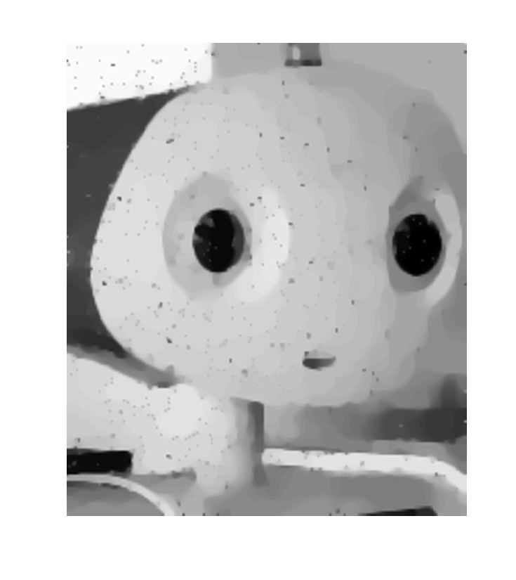
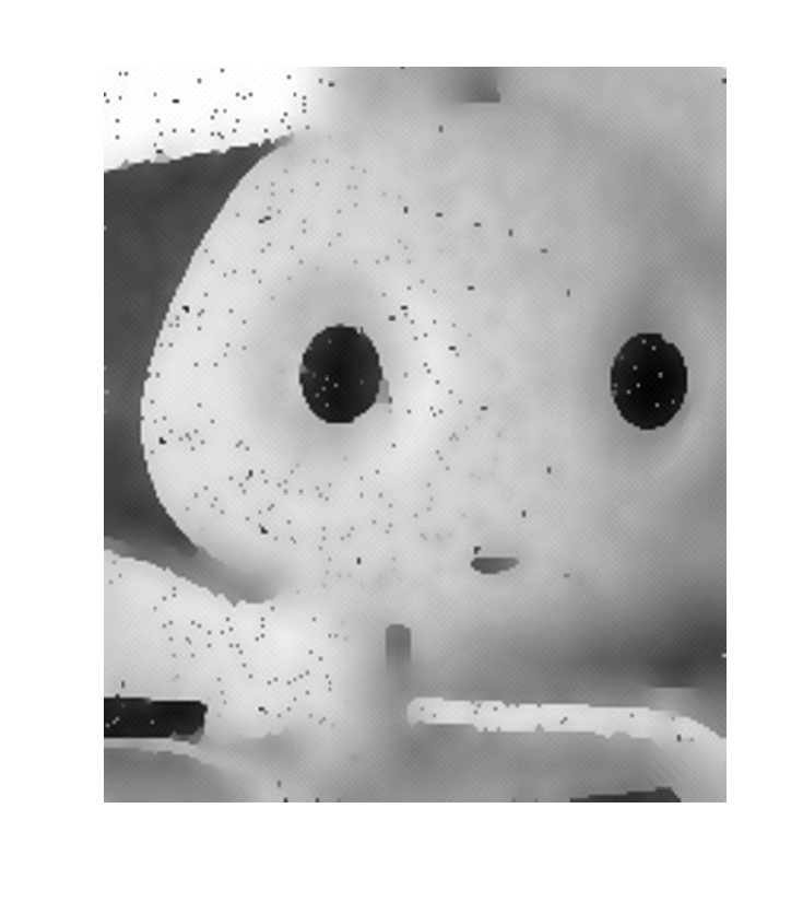
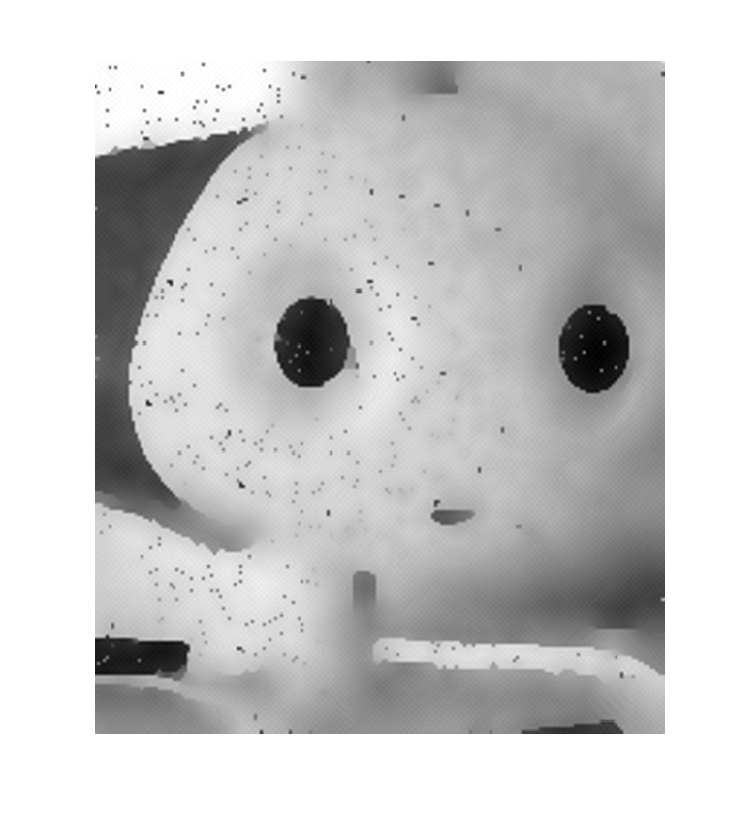
Let u¯\bar{u} be the noise-free image, see Fig. 1. In this paper, we consider two type of noise structure: (i) The uniformly distributed noise with noise level δ\delta (cf. (a) in Fig. 2). The noisy image is defined as u0δ​(x)=max⁡{0,[1+δ⋅(2​rand​(x)−1)]​u¯​(x)}u^{\delta}_{0}(x)=\max\{0,[1+\delta\cdot(2\,\textrm{rand}(x)-1)]\,\bar{u}(x)\}, x∈Ωx\in\Omega, where “rand” returns a pseudo-random value drawn from a uniform distribution on [0,1][0,1]. (ii) The salt and pepper dominated noise (cf. (b) in Fig. 2). It should be noted that for images with purely salt and pepper noise, specific approaches, such as median filtering methods ([Lim(1990)Lim, Juhola et al.(1998)Juhola, Katajainen, & Raita, Eng & Ma(2001)Eng & Ma, Eng, & Ma]), etc., work better than our proposed SV-DDF.

Refer to caption
Refer to caption
Figure 1: The two noise free images.
Refer to caption
Refer to caption
Figure 2: (a) Noisy image with uniformly distributed noise of level δ=54%\delta=54\%. (b) Noisy image with salt and pepper dominated noise.

To assess the accuracy of the denoised images we use the well known structural similarity error measure SSIM and the Peak Signal-to-Noise Ratio (PSNR) to obtain a quantitative estimate of the denoising performance ([Wang et al.(2004)Wang, Bovik, Sheikh, & Simoncelli]).

6.1 Influence of parameters

The purpose of this paragraph is to explore the dependence of the accuracy of the denoised image with respect to the damping parameter η\eta and the method parameter pp in order to find proper values in practice. In all simulations below, we set ϵ=σ=0.001\epsilon=\sigma=0.001. Numerical experiments indicate that small changes (less than 1%1\%) of the values of ϵ\epsilon and σ\sigma do not significantly influence the output of our method. In Tab. 1, we display the results by using different values of the damping parameter η\eta and the method parameter pp for the two noisy test images in Fig. 2. The results for the first test picture show that we obtain the best result for p=1p=1, η=300\eta=300 for both evaluation criteria of SSIM and PSNR. In the simulations of the second test picture, we also found that the optimal choice of pp still equals 1. However, for PSNR, the optimal value of damping parameter is much greater that the optimal η\eta for the first test picture. In both cases, a large value of damping parameter will not decrease the quality of denoised images significantly. Therefore, we recommend to set p=1p=1 and relative large value of damping parameter, e.g. η=300\eta=300, as the initial guess of parameters for our method in practice.

Table 1: Results with different damped parameters η\eta and pp; the table shows the SSIM value and PSNR value.
p∖ηp\setminus\eta 0.001 1 100 300 600 1500 3000
Picture (a) SSIM
1 0.108 0.108 0.538 0.549 0.548 0.548 0.548
1.5 0.116 0.116 0.114 0.530 0.532 0.532 0.532
2 0.032 0.032 0.032 0.032 0.032 0.081 0.135
Picture (a) PSNR
1 14.22 16.83 18.01 18.37 18.38 18.18 17.24
1.5 12.16 14.62 15.51 15.78 15.78 15.63 15.70
2 10.85 13.28 14.11 14.36 14.37 14.22 14.28
Picture (b) SSIM
1 0.366 0.374 0.482 0.697 0.752 0.754 0.753
1.5 0.403 0.487 0.541 0.683 0.748 0.748 0.747
2 0.107 0.108 0.291 0.359 0.383 0.403 0.462
Picture (b) PSNR
1 17.26 24.79 26.86 26.84 21.81 19.29 17.92
1.5 14.95 20.59 22.14 22.13 18.36 16.46 15.44
2 13.58 18.85 20.30 20.29 16.76 15.00 14.74

6.2 Comparison with other state-of-the-art methods

In order to show the advantages of our algorithm over existing approaches, we solve the same problem by the following methods: Total Variation (TV), Modified Telegraph (MTele, [Cao et al.(2010)Cao, Yin, Liu, & Li]), Telegraph (Tele, [Ratner & Zeevi(2013)Ratner & Zeevi]), Total Generalized Variation of the second order (TGV, [Bredies et al.(2010)Bredies, Kunisch, & Pock, Setzer et al.(2004)Setzer, Steidl, & Teuber]), and Median Filtering (MF, [Lim(1990)Lim]). In our MF method, each output pixel contains the median value in a 3-by-3 neighborhood around the corresponding pixel in the input image. In this group of simulations, we set η=300\eta=300 and η=1500\eta=1500 for the first and second test pictures respectively. Moreover, p=1p=1 for both test pictures.

Firstly, we compare the number of iterations required to reach a certain SSIM or PSNR by the five different iterative/dynamical denoising algorithms. The results are displayed in Table 2. Moreover, the evolutions of the SSIM value and PSNR value with respect to iterations for each method are shown in Figure 3, where one can see that unlike other four methods, whose SSIM and PSNR value are almost monotonic increasing, the SSIM/PSNR value of SV-DDF are oscillating during the evolutions. However, the trend of the SSIM/PSNR value for SV-DDF is to be a increasing function. By numerical simulations, which is omitted here, we found that the more oscillations of the SSIM/PSNR value of SV-DDF occur, the smaller the damping parameter η\eta in the model (6) is. This is an expected result due to the behaviour of damped Hamiltonian systems.

Table 2: Comparison of methods for a set final value of SSIM and PSNR.
SV-DDF TV MTele Tele TGV
Test picture (a) Iterations
Initial SSIM (Reached SSIM)
0.108 (0.400) 253 484 447 421 576
Initial PSNR (Reached PSNR)
12.07 (15.74) 227 592 476 468 524
Test picture (b) Iterations
Initial SSIM (Reached SSIM)
0.367 (0.435) 64 326 167 154 397
Initial PSNR (Reached PSNR)
18.81 (24.00) 67 492 129 124 502
Refer to caption
Refer to caption
Refer to caption
Refer to caption
Figure 3: Evolutions of the SSIM value and PSNR value with respect to iterations for the five iterative denoising algorithms: SV-DDF, TV, MTele, Tele and TGV.
Refer to caption
Refer to caption
Refer to caption
Noisy SV-DDF (504 iterations) TV (952 iterations)
SSIM: 0.108 SSIM: 0.549 SSIM: 0.549
PSNR: 12.07 PSNR: 18.37 PSNR: 18.35
Refer to caption
Refer to caption
Refer to caption
Original MTele (853 iterations) Tele (840 iterations)
SSIM: SSIM: 0.492 SSIM: 0.494
PSNR: PSNR: 16.48 PSNR: 16.17
Refer to caption
Refer to caption
TGV (680 iterations) MF
SSIM: 0.407 SSIM: 0.168
PSNR: 15.74 PSNR: 14.02
Figure 4: Test picture (a): results for the methods SV-DDF, TV, MTele, Tele, TGV and MF.

Next, we compare the qualities (the value of SSIM and PSNR) of the denoised images by the six mentioned algorithms. The results for two different types of noisy images are displayed in figures 4 and 5 respectively, where in each figure the test degraded image is given in the first picture, while the exact image and the denoised images are displayed in the last seven pictures. We see that for text image (a), the SV-DDF, as well as the TV method, gives the highest SSIM value 0.549, and also gives a smoother result than the other methods. However, the PSNR value of SV-DDF is slightly higher than the PSNR value of TV. Moreover, the TV method requires much more iterations to reach the result. For test image (b), the SV-DDF method presents the best results among all methods both regarding quality measures and iterations. However, as shown in figure 5, for image (b), like the TV method, our SV-DDF also exhibit the staircasing phenomenon. It is well known that the TGV methods do not lead to a staircasing effect, which motivates us to develop a new second order flow with TGV gradient, i.e.

ut​t+η​ut−TGVα2​(u)=0,u⁡(x,0)=u0​(x),ut​(x,0)=0​ in ​Ω,u_{tt}+\eta u_{t}-\textmd{TGV}^{2}_{\alpha}(u)=0,\quad u(x,0)=u_{0}(x),u_{t}(x,0)=0\textmd{~in~}\ \Omega, (50)

where the definition of TGVα2​(⋅)\textmd{TGV}^{2}_{\alpha}(\cdot), i.e. the total generalized bounded variation of order 2 with weight α\alpha, can be found in ([Bredies et al.(2010)Bredies, Kunisch, & Pock, Setzer et al.(2004)Setzer, Steidl, & Teuber]). Similar as SV-DDF in (46), one can propose a discretized version of second order flow (50) (we denote it as SV-DDF-TGV). The result of SV-DDF-TGV for nosiy image (b) is displayed in the last picture of Figure 5, where we see that there is no staircase artifact for SV-DDF-TGV. However, the quality (both of value of SSIM and PSNR) of SV-DDF-TGV is much worse than the quality of the original SV-DDF method. Moreover, the well-posedness of the second order flow (50), i.e. the existence, uniqueness, and regularization property of DF, are still open questions.

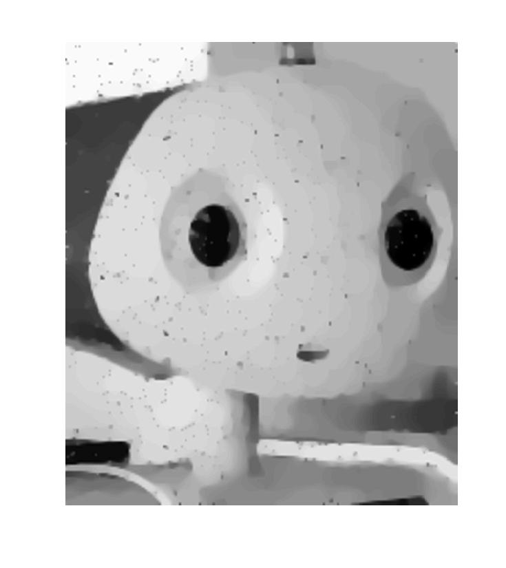
Refer to caption
Refer to caption
Refer to caption
Noisy SV-DDF (138 iterations) TV (1726 iterations)
SSIM: 0.367 SSIM: 0.754 SSIM: 0.742
PSNR: 18.81 PSNR: 26.84 PSNR: 26.20
Refer to caption
Refer to caption
Refer to caption
Original MTele (799 iterations) Tele (773 iterations)
SSIM: SSIM: 0.561 SSIM: 0.559
PSNR: PSNR: 24.17 PSNR: 24.16
Refer to caption
Refer to caption
Refer to caption
TGV (687 iterations) MF SV-DDF-TGV (87 iterations)
SSIM: 0.435 SSIM: 0.282 SSIM: 0.503
PSNR: 24.67 PSNR: 23.82 PSNR: 25.53
Figure 5: Test picture (b): results for the methods SV-DDF, TV, MTele, Tele, TGV, MF and SV-DDF-TGV.

7 Conclusion.

In this paper, we introduce a new image denoising model – the damped flow. The existence and uniqueness of the solution to the model are both proven under certain assumptions. For the numerical implementation, based on the Störmer-Verlet method, a discrete damped flow, SV-DDF, is developed. The convergence of SV-DDF is discussed as well. A numerical algorithm with automatic stopping criterion is provided. A comparison with three existing methods show that the SV-DDF appears to be very competitive with respect to its image denoising capabilities and its acceleration affect. Obviously, beside in the pp-Dirichlet energy denoising, the damped flow can also be used for solving a general non-linear optimization problem of the type (1), see e.g. the denoising model (50). Finally, we emphasis that the aim of the paper is to introduce the SV-DDF method to image denoising. Since it is comparable to the conventional TV method, it is a promising approach which merits further theoretical and numerical development as well as more extensive comparison to state-of-the-art methods.

Acknowledgment

We express our gratitude to the associate editor and two anonymous reviewers whose valuable comments and suggestions lead to an improvement of the manuscript.

The work of Y. Zhang is supported by the Alexander von Humboldt foundation through a postdoctoral researcher fellowship.

References

  • [Adams & Fournier(2003)Adams & Fournier] Adams, R. & Fournier, J. (2003) Sobolev spaces, vol. 140. Cambridge: Academic press.
  • [Alvarez(2000)Alvarez] Alvarez, F. (2000) On the minimizing property of a second-order dissipative system in hilbert spaces. SIAM J. Control Optim., 38, 1102–1119.
  • [Alvarez et al.(2002)Alvarez, Attouch, Bolte, & Redont] Alvarez, F., Attouch, H., Bolte, J. & Redont, P. (2002) A second-order gradient-like dissipative dynamical system with hessian-driven damping. application to optimization and mechanics. J. Math. Pures Appl., 81, 747–779.
  • [Alvarez et al.(1992)Alvarez, Lions, & Morel] Alvarez, L., Lions, P. & Morel, J. (1992) Image selective smoothing and edge detection by nonlinear diffusion (ii). SIAM J. Numer. Anal., 29, 845–866.
  • [Alvarez et al.(1993)Alvarez, Guichard, Lions, & Morel] Alvarez, L., Guichard, F., Lions, P. & Morel, J. (1993) Axioms and fundamental equations of image processing. Archive for Rational Mechanics and Analysis, 123, 199–257.
  • [Åström et al.(2017)Åström, Felsberg, & Baravdish] Åström, F., Felsberg, M. & Baravdish, G. (2017) Mapping-based image diffusion. J. Math. Imaging Vis., 57, 293–323.
  • [Attouch et al.(2000)Attouch, Goudou, & Redont] Attouch, H., Goudou, X. & Redont, P. (2000) The heavy ball with friction method. i. the continuous dynamical system. Comm. Contemp. Math., 2, 1–34.
  • [Baravdish et al.(2015)Baravdish, Svensson, & Åström] Baravdish, G., Svensson, O. & Åström, F. (2015) On Backward p(x)-Parabolic Equations for Image Enhancement. Numer. Func. Anal. Opt., 36, 147–168.
  • [Bollt et al.(2009)Bollt, Chartrand, Esedolu, Schultz, & Vixie] Bollt, E., Chartrand, R., Esedolu, S., Schultz, P. & Vixie, K. (2009) Graduated adaptive image denoising: local compromise between total variation and isotropic diffusion. Adv. Comput. Math., 31, 61–85.
  • [Bredies et al.(2010)Bredies, Kunisch, & Pock] Bredies, K., Kunisch, K. & Pock, T. (2010) Total generalized variation. SIAM J. Imaging Sci., 3, 492–526.
  • [Cao et al.(2010)Cao, Yin, Liu, & Li] Cao, Y., Yin, J., Liu, Q. & Li, M. (2010) A class of nonlinear parabolic-hyperbolic equations applied to image restoration. Nonlinear Anal-Real., 11, 253–261.
  • [Catté et al.(1992)Catté, Lions, Morel, & Coll] Catté, F., Lions, P., Morel, J. & Coll, T. (1992) Image selective smoothing and edge detection by nonlinear diffusion. SIAM J. Numer. anal., 29, 182–193.
  • [Chen et al.(2006)Chen, Levine, & Rao] Chen, Y., Levine, S. & Rao, M. (2006) Variable exponent, linear growth functionals in image restoration. SIAM J. Appl. Math., 66, 1383–1406.
  • [DiBenedetto(1993)DiBenedetto] DiBenedetto, E. (1993) Degenerate Parabolic Equations. Berlin: Springer New York.
  • [Donoho & Johnstone(1995)Donoho & Johnstone] Donoho, D. & Johnstone, I. (1995) Adapting to unknown smoothness via wavelet shrinkage. J. Am. Stat. Assoc., 90, 1200–1224.
  • [Edvardsson et al.(2012)Edvardsson, Gulliksson, & Persson] Edvardsson, S., Gulliksson, M. & Persson, J. (2012) The dynamical functional particle method: an approach for boundary value problems. J. Appl. Mech., 79, 021012.
  • [Edvardsson et al.(2015)Edvardsson, Neuman, Edström, & Olin] Edvardsson, S., Neuman, M., Edström, P. & Olin, H. (2015) Solving equations through particle dynamics. Comput. Phys. Commun., 197, 169–181.
  • [Eng & Ma(2001)Eng & Ma, Eng, & Ma] Eng, H. & Ma, K. (2015) Noise adaptive soft-switching median filter. IEEE Trans. Image Process., 10, 242–251.
  • [Evans(2010)Evans] Evans, L. (2010) Partial differential equations, vol. 19. Providence: American Mathematical Society.
  • [Gonzalez & Woods(2007)Gonzalez & Woods] Gonzalez, R. & Woods, R. (2007) Digital Image Processing (3rd Edition). New Jersey: Prentice Hall.
  • [Gong et al.(2019)Rong, Hofmann, & Zhang] Gong, R., Hofmann, B. & Zhang, Y. (2018) A new class of accelerated regularization methods, with application to bioluminescence tomography. arXiv:1903.05972.
  • [Grasmair & Lenzen(2010)Grasmair & Lenzen] Grasmair, M. & Lenzen, F. (2010) Anisotropic total variation filtering. Applied Mathematics & Optimization, 62, 323–339.
  • [Hairer et al.(2006)Hairer, Wanner, & Lubich] Hairer, E., Wanner, G. & Lubich, C. (2006) Geometric Numerical Integration: Structure-Preserving Algorithms for Ordinary Differential Equations (Second Edition). New York: Springer.
  • [Hanke et al.(1995)Hanke, Neubauer, & Scherzer] Hanke, M., Neubauer, A. & Scherzer, O. (1995) A convergence analysis of the Landweber iteration for nonlinear ill-posed problems. Numerische Mathematik, 72, 21–37.
  • [Haraux & Jendoubi(2007)Haraux & Jendoubi] Haraux, A. & Jendoubi, M. (2007) On the convergence of global and bounded solutions of some evolution equations. J. Evol. Equ., 7, 449–470.
  • [Haraux & Zuazua(1988)Haraux & Zuazua] Haraux, A. & Zuazua, E. (1988) Decay estimates for some semilinear damped hyperbolic problems. Arch. Ration. Mech. An., 100, 191–206.
  • [Hochbruck et al.(1998)Hochbruck, Lubich, & Selhofer] Hochbruck, M., Lubich, C. & Selhofer, H. (1998) Exponential integrators for large systems of differential equations. SIAM J. Sci. Comput., 19, 1152–1174.
  • [Juhola et al.(1998)Juhola, Katajainen, & Raita] Juhola, M., Katajainen, J. & Raita, T. (1991) Comparison of algorithms for standard median filtering. IEEE Trans. Signal Process, 39, 204–208.
  • [Khanian et al.(2014)Khanian, Feizi, & Davari] Khanian, M., Feizi, A. & Davari, A. (2014) An optimal partial differential equations-based stopping criterion for medical image denoising. J Med Signals Sens., 4, 72–83.
  • [Kuijper(2009)Kuijper] Kuijper, A. (2009) Geometrical PDEs based on second-order derivatives of gauge coordinates in image processing. Image Vision Comput., 27, 1023–1034.
  • [Ladyzhenskaja et al.(1988)Ladyzhenskaja, Solonnikov, & Uraltseva] Ladyzhenskaja, O., Solonnikov, V. & Uraltseva, N. (1988) Linear and quasi-linear equations of parabolic type. Providence: American Mathematical Society.
  • [Lieberman(1996)Lieberman] Lieberman, G. (1996) Second order parabolic differential equations. Singapore: World scientific.
  • [Lim(1990)Lim] Lim, Jae S. (1990) Two-Dimensional Signal and Image Processing. New Jersey: Prentice Hall.
  • [Perona & Malik(1990)Perona & Malik] Perona, P. & Malik, J. (1990) Scale-space and edge detection using anisotropic diffusion. IEEE Transactions on Pattern Analysis and Machine Intelligence, 12, 629–639.
  • [Preusser et al.(2008)Preusser, Scharr, Krajsek, & Kirby] Preusser, T., Scharr, H., Krajsek, K. & Kirby, R. (2008) Building blocks for computer vision with stochastic partial differential equations. Int. J. Comput. Vision, 80, 375–405.
  • [Ratner & Zeevi(2011)Ratner & Zeevi] Ratner, V. & Zeevi, Y. (2011) Denoising-enhancing images on elastic manifolds. IEEE Trans. Image Proc., 20, 2099–2109.
  • [Ratner & Zeevi(2013)Ratner & Zeevi] Ratner, V. & Zeevi, Y. (2013) Stable denoising-enhancement of images by telegraph-diffusion operators image processing. in ICIP 2013 Proc. IEEE, 1252–1256.
  • [Rieder(2005)Rieder] Rieder, A. (2005) Runge-Kutta integrators yield optimal regularization schemes. Inverse Problems, 21, 453–471.
  • [Roubíček(2013)Roubíček] Roubíček, T. (2013) Nonlinear partial differential equations with applications, vol. 153. Berlin: Springer Science & Business Media.
  • [Rudin et al.(1992)Rudin, Osher, & Fatemi] Rudin, L., Osher, S. & Fatemi, E. (1992) Nonlinear total variation based noise removal algorithms. Physica D: Nonlinear Phenomena, 60, 259–268.
  • [Sandin et al.(2016)Sandin, Ögren, & Gulliksson] Sandin, P., Ögren, M. & Gulliksson, M. (2016) Numerical solution of the stationary multicomponent nonlinear schrodinger equation with a constraint on the angular momentum. Phys. Rev. E, 93, 033301.
  • [Scherzer et al.(2009)Scherzer, Grasmair, Grossauer, Haltmeier, & Lenzen] Scherzer, O., Grasmair, M., Grossauer, H., Haltmeier, M. & Lenzen, F. (2009) Variational Methods in Imaging. Berlin: Springer.
  • [Setzer et al.(2004)Setzer, Steidl, & Teuber] Setzer, S., Steidl, G., & Steidl, T. (2011) Infimal convolution regularizations with discrete l1l_{1}-type functionals, Commun. in Math. Sci., 9, 797–827.
  • [Tadmor(2012)Tadmor] Tadmor, E. (2012) A review of numerical methods for nonlinear partial differential equations. Bulletin Amer. Math. Soc., 49, 507–554.
  • [Tautenhahn(1994)Tautenhahn] Tautenhahn, U. (1994) On the asymptotical regularization of nonlinear ill-posed problems. Inverse Problems, 10, 1405–1418.
  • [Wang et al.(2004)Wang, Bovik, Sheikh, & Simoncelli] Wang, Z., Bovik, A., Sheikh, H. & Simoncelli, E. (2004) Image quality assessment: from error visibility to structural similarity. IEEE Transactions on Image Processing, 13, 600–612.
  • [Weickert(1998)Weickert] Weickert, J. (1998) Anisotropic diffusion in image processing. Stuttgart: Teubner-Verlag.
  • [Wu et al.(2001)Wu, Yin, Li, & Zhao] Wu, Z., Yin, J., Li, H. & Zhao, J. (2001) Nonlinear diffusion equations. Singapore: World Scientific.
  • [Zhang et al.(2018)Zhang, Gong, Cheng, & Gulliksson] Zhang, Y., Gong, R., Cheng, X. & Gulliksson, M. (2018) A dynamical regularization algorithm for solving inverse source problems of elliptic partial differential equations. Inverse Problems, 34, 065001.
  • [Zhang & Hofmann(2018)Zhang & Hofmann] Zhang, Y. & Hofmann, B. (2018) On the second order asymptotical regularization of linear ill-posed inverse problems. Appl. Anal., DOI, 10.1080/00036811.2018.1517412.
  • [Zhang & Hofmann(2019)Zhang & Hofmann] Zhang, Y. & Hofmann, B. (2019) On fractional asymptotical regularization of linear ill-posed problems in Hilbert spaces. Fract. Calc. Appl. Anal., 22, 699–721.