pt
Segmentation of Photovoltaic Module Cells in Uncalibrated Electroluminescence Images
Abstract
High resolution electroluminescence (EL) images captured in the infrared spectrum allow to visually and non-destructively inspect the quality of photovoltaic (PV) modules. Currently, however, such a visual inspection requires trained experts to discern different kinds of defects, which is time-consuming and expensive. Automated segmentation of cells is therefore a key step in automating the visual inspection workflow.
In this work, we propose a robust automated segmentation method for extraction of individual solar cells from EL images of PV modules. This enables controlled studies on large amounts of data to understanding the effects of module degradation over time—a process not yet fully understood.
The proposed method infers in several steps a high-level solar module representation from low-level ridge edge features. An important step in the algorithm is to formulate the segmentation problem in terms of lens calibration by exploiting the plumbline constraint. We evaluate our method on a dataset of various solar modules types containing a total of solar cells with various defects. Our method robustly solves this task with a median weighted Jaccard index of and an score of , both indicating a high sensitivity and a high similarity between automatically segmented and ground truth solar cell masks.
Keywords:
PV modules, EL imaging, visual inspection, lens distortion, solar cell extraction, pixelwise classification1 Introduction
Visual inspection of solar modules using EL imaging allows to easily identify damage inflicted to solar panels either by environmental influences such as hail, during the assembly process, or due to prior material defects or material aging Nian et al. (2010); Breitenstein et al. (2011); Tsai et al. (2012); Tsai et al. (2013); Anwar and Abdullah (2014); Tseng et al. (2015). The resulting defects can notably decrease the photoelectric conversion efficiency of the modules and thus their energy yield. This can be avoided by continuous inspection of solar modules and maintenance of defective units. For an introduction and review of non-automatic processing tools for EL images, we refer to Mauk (2013).
An important step towards an automated visual inspection is the segmentation of individual cells from the solar module. An accurate segmentation allows to extract spatially normalized solar cell images. We already used the proposed method to develop a public dataset of solar cells images Buerhop-Lutz et al. (2018), which are highly accurate training data for classifiers to predict defects in solar modules Deitsch et al. (2019); Mayr et al. (2019). In particular, the Convolutional Neural Network (CNN) training is greatly simplified when using spatially normalized samples, because CNNs are generally able to learn representations that are only equivariant to small translations (Goodfellow et al., 2016, pp. 335–336). The learned representations, however, are not naturally invariant to other spatial deformations such as rotation and scaling Goodfellow et al. (2016); Jaderberg et al. (2015); Lin and Lucey (2017).
The identification of solar cells is additionally required by the international technical specification IEC TS 60904-13 (IEC TS 60904-13:2018, 2018, Annex D) for further identification of defects on cell level. Automated segmentation can also ease the development of models that predict the performance of a PV module based on detected or identified failure modes, or by determining the operating voltage of each cell Potthoff et al. (2010). The data describing the cell characteristics can be fed into an electric equivalent model that allows to estimate or simulate the current-voltage characteristic (I-V) curve Quaschning and Hanitsch (1996); Chenni et al. (2007); Karatepe et al. (2007) or even the overall power output Kaushika and Gautam (2003).

The appearance of PV modules in EL images depends on a number of different factors, which makes an automated segmentation challenging. The appearance varies with the type of semiconducting material and with the shape of individual solar cell wafers. Also, cell cracks and other defects can introduce distracting streaks. A solar cell completely disconnected from the electrical circuit will also appear much darker than a functional cell. Additionally, solar modules vary in the number of solar cells and their layout, and solar cells themselves are oftentimes subdivided by busbars into multiple segments of different sizes. Therefore, it is desirable for a fully automated segmentation to infer both the arrangement of solar cells within the PV module and their subdivision from EL images alone, in a way that is robust to various disturbances. In particular, this may ease the inspection of heterogeneous batches of PV modules.
In this work, we assume that EL images are captured in a manufacturing setting or under comparable conditions in a test laboratory where field-aged modules are analyzed either regularly or after hazards like hailstorms. Such laboratories oftentimes require agile work processes where the equipment is frequently remounted. In these scenarios, the EL irradiation of the solar module predominates the background irradiation, and the solar modules are captured facing the EL camera without major perspective distortion. Thus, the geometric distortions that are corrected by the proposed method are radial lens distortion, in-plane rotation, and minor perspective distortions. This distinguishes the manufacturing setting from acquisitions in the field, where PV modules may be occluded by cables and parts of the rack, and the perspective may be strong enough to require careful correction. However, perspective distortion also makes it more difficult to identify defective areas (e.g., microcracks) due to the foreshortening effect Aloimonos (1988). Therefore, capturing EL images from an extreme perspective is generally not advisable. Specifically for manufacturing environments, however, the proposed method yields a robust, highly accurate, and completely automatic segmentation of solar modules into solar cells from high resolution EL images of PV modules.
Independently of the setting, our goal is to allow for some flexibility for the user to freely position the camera or use zoom lenses without the need to recalibrate the camera.
With this goal in mind, a particular characteristic of the proposed segmentation pipeline is that it does not require an external calibration pattern. During the detection of the grid that identifies individual solar cells, the busbars and the inter solar cell borders are directly used to estimate lens distortion. Avoiding the use of a separate calibration pattern also avoids the risk of an operator error during the calibration, e.g., due to inexperienced personnel.
A robust and fully automatic PV module segmentation can help understanding the influence of module degradation on module efficiency and power generation. Specifically, this allows to continuously and automatically monitor the degradation process, for instance, by observing the differences in a series of solar cell images captured over a certain period of time. The segmentation also allows to automatically create training data for learning-based algorithms for defect classification and failure prediction.
1.1 Contributions
To the best of our knowledge, the proposed segmentation pipeline is the first work to enable a fully automatic extraction of solar cells from uncalibrated EL images of solar modules (cf., ). Within the pipeline, we seek to obtain the exact segmentation mask of each solar cell through estimation of non-linear and linear transformations that warp the EL image into a canonical view. To this end, our contributions are three-fold:
- 1.
Joint camera lens distortion estimation and PV module grid detection for precise solar cell region identification.
- 2.
A robust initialization scheme for the employed lens distortion model.
- 3.
A highly accurate pixelwise classification into active solar cell area on monocrystalline and polycrystalline PV modules robust to various typical defects in solar modules.
Moreover, our method operates on arbitrary (unseen) module layouts without prior knowledge on the layout.
1.2 Outline
The remainder of this work is organized as follows. Section 2 discusses the related work. In Section 3, the individual stages of the segmentation pipeline are presented. In Section 4, we evaluate the presented segmentation approach on a number of different PV modules with respect to the segmentation accuracy. Finally, the conclusions are given in Section 5.
2 Related Work
The segmentation of PV modules into individual solar cells is related to the detection of calibration patterns, such as checkerboard patterns commonly used for calibrating intrinsic camera and lens parameters Rufli et al. (2008); Placht et al. (2014); Fürsattel et al. (2016); Hoffmann et al. (2017); Ha et al. (2017). However, the appearance of calibration patterns is typically perfectly known, whereas detection of solar cells is encumbered by various defects that are a priori unknown. Additionally, the number of solar cells in a PV module and their layout can vary. We also note that existing lens models generally assume wide angle lenses. However, their application to standard lenses is to our knowledge not widely studied.
To estimate the parameters of a lens distortion model, the plumbline constraint is typically employed Brown (1971). The constraint exploits the fact that the projection of straight lines under radial and tangential distortion will not be truly straight. For example, under radial distortion, straight lines are images as curves. For typical visual inspection tasks, a single image is sufficient to estimate the lens distortion parameters Devernay and Faugeras (2001); Fitzgibbon (2001); Claus and Fitzgibbon (2005a); Ahmed and Farag (2005); Claus and Fitzgibbon (2005b); Rosten and Loveland (2011). This can be achieved by decoupling the intrinsic parameters of the camera from the parameters of the lens distortion model Devernay and Faugeras (2001).
Novel methodologies employ CNNs for various segmentation tasks. Existing CNN-based segmentation tasks can be categorized into (1) object detection, (2) semantic segmentation, and (3) instance-aware segmentation. One of the first CNN object detection architectures is Regions with CNN features (R-CNN) Girshick et al. (2014) to learn features that are subsequently classified using a class-specific linear Support Vector Machine (SVM) to generate region proposals. R-CNN learns to simultaneously classify object proposals and refine their spatial locations. The predicted regions, however, provide only a coarse estimation of object’s location in terms of bounding boxes. Girshick (2015) proposed Fast Region-based Convolutional Neural Network (Fast R-CNN) by accelerating training and testing times while also increasing the detection accuracy. Ren et al. (2017) introduced Region Proposal Network (RPN) that shares full-image convolutional features with the detection network enabling nearly cost-free region proposals. RPN is combined with Fast R-CNN into a single network that simultaneously predicts object bounds and estimates the probability of an object for each proposal. For semantic segmentation, Long et al. (2015) introduced Fully Convolutional Networks (FCNs) allowing for pixelwise inference. The FCN is learned end-to-end and pixels-to-pixels requiring appropriately labeled training data. Particularly, in medical imaging the U-Net network architecture by Ronneberger et al. (2015) has been successfully applied for various segmentation tasks. In instance segmentation, Li et al. (2017) combined segment proposal and object detection for Fully Convolutional Instance Segmentation (FCIS) where the general idea is to predict the locations in a fully convolutional network. He et al. (2017) proposed a Mask R-CNN which extends Faster R-CNN.
The work by Mehta et al. (2018) introduces a CNN for the prediction of power loss. Their system additionally localizes and classifies the type of soiling. Their work is based on RGB images of whole PV modules and addresses the additional geometric challenges of acquisitions in the field. In contrast, this work operates on EL images of individual cells of a PV module, and in particular focuses on their precise segmentation in a manufacturing setting.
The main limitation of learning-based approaches is the requirement of a considerable number of appropriately labeled images for training. However, pixelwise labeling is time-consuming, and in absence of data not possible at all. Also, such learning-based approaches require training data that is statistically representative for the test data, which oftentimes requires to re-train a model on data with different properties. In contrast, the proposed approach can be readily deployed to robustly segment EL images of PV modules without notable requirements of labeled training data.
The closest work related to the proposed method was presented by Sovetkin and Steland (2019). This method proposes a robust PV module grid alignment for the application on field EL images, where radial and perspective distortion, motion blur, and disturbing background may be present. The method uses an external checkerboard calibration for radial distortion correction, and prior knowledge on the solar cell topology in terms of the relative distances of the grid lines separating the busbars and cell segments. In contrast, EL images taken under manufacturing conditions may be cropped or rotated, and the camera is not always pre-calibrated. Hence, the proposed method performs an automated on-line calibration for every EL image. This is particularly useful for EL images of PV modules from various sources, for which the camera parameters may not be available, or when zoom lenses are used. Additionally, the proposed method performs a pixelwise classification of pixels belonging to the active cell area and therefore is able to provide masks tailored to a specific module type. Such masks allow to exclude unwanted background information and to simplify further processing.
In this work, we unify lens distortion estimation and grid detection by building upon ideas of Devernay and Faugeras (2001). However, instead of using independent line segments to estimate lens distortion parameters, we constrain the problem using domain knowledge by operating on a coherent grid. This joint methodology allows to correct errors through feedback from the optimization loop used for estimating lens model parameters. The proposed approach conceptually differs from Sovetkin and Steland (2019), where both steps are decoupled and an external calibration is required.
3 Methodology
The proposed framework uses a bottom-up pipeline to gradually infer a high-level representation of a solar module and its cells from low-level ridge edge features in an EL image. Cell boundaries and busbars are represented as parabolic curves to robustly handle radial lens distortion which causes straight lines to appear curved in the image. Once we estimated the lens distortion parameters, the parabolas are rectified to obtain a planar cell grid. This rectified representation is used to segment the solar cells.
3.1 Overview
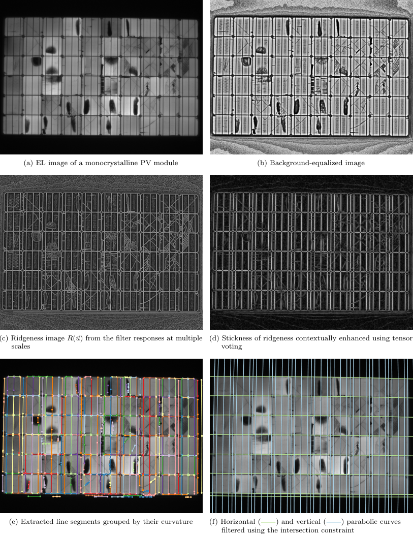
The general framework for segmenting the solar cells in EL images of PV modules is illustrated in Fig. 2 and consists of the following steps. First, we locate the busbars and the inter solar cell borders by extracting the ridge edges. The ridge edges are extracted at subpixel accuracy and approximated by a set of smooth curves defined as second-degree polynomials. The parametric representation is used to construct an initial grid of perpendicularly arranged curves that identify the PV module. Using this curve grid, we estimate the initial lens distortion parameters and hypothesize the optimal set of curves by further excluding outliers in a RANdom SAmple Consensus (RANSAC) scheme. Then we refine the lens distortion parameters that we eventually use to rectify the EL image. From the final set of curves we infer the PV module configuration and finally extract the size, perspective, and orientation of solar cells.
3.2 Preprocessing
First, the contrast of an EL image is enhanced to account for possible underexposure. Then, low-level edge processing is applied to attenuate structural variations that might stem from cracks or silicon wafer texture, with the goal of preserving larger lines and curves.
3.2.1 Contrast Enhancement
Here, we follow the approach by Franken et al. (2006b). A copy of the input EL image is blurred with a Gaussian kernel, and a morphological closing with a disk-shaped structure element is applied. Dividing each pixel of by attenuates unwanted background noise while emphasizing high contrast regions. Then, histogram equalization (Gonzalez and Woods, 2018, pp. 134 sqq.) is applied to increase its overall contrast. shows the resulting image .
3.2.2 Gaussian Scale-Space Ridgeness
The high-level grid structure of a PV module is defined by inter-cell borders and busbars, which correspond to ridges in the image. Ridge edges can be determined from second-order partial derivatives summarized by a Hessian. To robustly extract line and curve ridges, we compute the second-order derivative of the image at multiple scales Lindeberg (1996); Lindeberg (1998). The responses are computed in a Gaussian pyramid constructed from an input EL image Lindeberg (1994). This results in several layers of the pyramid at varying resolutions commonly referred to as octaves. The eigendecomposition of the Hessian computed afterwards provides information about line-like structures.
More in detail, let denote discrete pixel coordinates, the number of octaves in the pyramid, and the number of sublevels in each octave. At the finest resolution, we set to the golden ratio . At each octave and sublevel , we compute the Hessian by convolving the image with the derivatives of the Gaussian kernel. To obtain the eigenvalues, the symmetric Hessian is diagonalized by annihilating the off-diagonal elements using the Jacobi method which iteratively applies Givens rotations to the matrix Golub and Van Loan (2013). This way, its eigenvalues and the corresponding eigenvectors can be simultaneously extracted in a numerically stable manner. Let denote the eigendecomposition of the Hessian , where is a diagonal matrix of eigenvalues and are the associated eigenvectors. Under a Gaussian assumption, the leading eigenvector dominates the likelihood if the associated leading eigenvalue is spiked. In this sense, the local ridgeness describes the likelihood of a line segment in the image at position , and the orientation of the associated eigenvector specifies the complementary angle of the most likely line segment orientation at position . The local ridgeness is obtained as the maximum positive eigenvalue across all octaves and sublevels. Both the ridgeness and the angle provide initial cues for ridge edges in the EL image (see ).
3.2.3 Contextual Enhancement via Tensor Voting
Ridgeness can be very noisy (cf., ). To discern noise and high curvatures from actual line and curve features, is contextually enhanced using tensor voting Medioni et al. (2000).
Tensor voting uses a stick tensor voting field to model the likelihood that a feature in the neighborhood belongs to the same curve as the feature in the origin of the voting field Franken et al. (2006a). The parameter controls the proximity of the voting field, and determines the angular specificity that we set to in our experiments.
Following Franken et al. (2006a), stickness is computed as the difference between the two eigenvalues of the tensor field, where . is the angle of the eigenvector associated with the largest eigenvalue , analogously to .
We iterate tensor voting two times, since one pass is not always sufficient Franken et al. (2006b). Unlike Franken et al., however, we do not thin out the stickness immediately after the first pass to avoid too many disconnected edges. Given the high resolution of the EL images in our dataset of approximately pixels, we use a fairly large proximity of in the first tensor voting step, and in the second.
shows a typical stickness output. The stickness along the orientation is used to extract curves at subpixel accuracy in the next step of the pipeline.
3.3 Curve Extraction
We seek to obtain a coherent grid which we define in terms of second-degree curves. These curves are traced along the previously extracted ridges by grouping centerline points by their curvature. We then fit second-degree polynomials to these points, which yields a compact high-level curve representation while simultaneously allowing to discard point outliers.
3.3.1 Extraction of Ridges at Subpixel Accuracy
To ensure a high estimation accuracy of lens distortion parameters, we extract ridge edges at subpixel accuracy. This also makes the segmentation more resilient in out-of-focus scenarios, where images may appear blurry and the ridge edges more difficult to identify due to their smoother appearance. Blurry images can be caused by slight camera vibrations during the long exposure time of several seconds that is required for imaging. Additionally, focusing in a dark room can be challenging, hence blur cannot be always avoided. Nevertheless, it is beneficial to be able to operate also on blurry images, as they can still be useful for defect classification and power yield estimation in cell areas that do not irradiate.
To this end, we perform non-maximum suppression by Otsu’s global thresholding Otsu (1979) on the stickness followed by skeletonization Saeed et al. (2010). Afterwards, we collect the points that represent the centerline of the ridges through edge linking Kovesi (2017). The discrete coordinates can then be refined by setting the centerline to the mean of a Gaussian function fitted to the edge profile Fabijańska (2012) using the Gauss-Newton (GN) optimization algorithm Nocedal and Wright (2006). The 1-dimensional window of the Gaussian is empirically set to 21 pixels, with four sample points per pixel that are computed via bilinear interpolation. The GN algorithm is initialized with the sample mean and standard deviation in the window, and multiplicatively scaled to the stickness magnitude at the mean. The mean of the fitted Gaussian is then reprojected along the edge profile oriented at to obtain the edge subpixel position. Figure 3 visualizes these steps.
A non-parametric alternative to fitting a Gaussian to the ridge edge profile constitutes fitting a parabola instead Devernay (1995). Such an approach is very efficient since it involves a closed-form solution. On the downside, however, the method suffers from oscillatory artifacts which require additional treatment Grompone von Gioi and Randall (2017).
3.3.2 Connecting Larger Curve Segments
A limitation of the edge linking method is that it does not prioritize curve pairs with similar orientation. To address this, we first reduce the set of points that constitute a curve to a sparse representation using the non-parametric variant of the Ramer-Douglas-Peucker algorithm Ramer (1972); Douglas and Peucker (1973) introduced by Prasad et al. (2012). Afterwards, edges are disconnected if the angle between the corresponding line segments is nonzero. In a second pass, two line segments are joined if they are nearby, of approximately the same length, and pointing into the same direction within an angle range . Figure 4 illustrates the way two curve segments are combined.
In the final step, the resulting points of the -th curve of a line segment form a matrix . For brevity, we denote the -th column of by . is used to find the parametric curve representation.
3.3.3 Parametric Curve Representation
Projected lines are represented as second-degree polynomials to model radial distortion. The curve parameters are computed via linear regression on the curve points. More specifically, let
| (1) |
denote a second-degree polynomial in horizontal or vertical direction. The curve is fitted to line segment points of the -th curve by minimizing the Mean Squared Error (MSE)
| (2) |
using RANSAC iterations Fischler and Bolles (1981). In one iteration, we randomly sample three points to fit Eq. 1, and then determine which of the remaining points support this curve model via MSE. Outlier points are discarded if the squared difference between the point and the parabolic curve value at its position exceeds . To keep the computational time low, RANSAC is limited to iterations, and stopped early once sufficiently many inliers at a confidence level are found (Hartley and Zisserman, 2004, ch. 4.7). After discarding the outliers, each curve is refitted to supporting candidate points using linear least squares Golub and Van Loan (2013). To ensure a numerically stable and statistically robust fit, the 2-D coordinates are additionally normalized Harker et al. (2008).
3.4 Curve Grid Model Estimation
The individual curves are used to jointly form a grid, which allows to further discard outliers, and to estimate lens distortion. To estimate the lens distortion, we employ the plumbline constraint Brown (1971). The constraint models the assumption that curves in the image correspond to straight lines in real world. In this way, it becomes possible to estimate distortion efficiently from a single image, which allows to use this approach also post hoc on cropped, zoomed or similarly processed images.
3.4.1 Representation of Lens Distortion
Analogously to Devernay and Faugeras (2001), we represent the radial lens distortion by a function that maps the distance of a pixel from the distortion center to a distortion factor. This factor can be used to radially displace each normalized image coordinate .
Image coordinates are normalized by scaling down coordinates horizontally by the distortion aspect ratio (corresponding to image aspect ratio decoupled from the projection on the image plane) followed by shifting the center of distortion to the origin and normalizing the resulting 2-D point to the unit range using the dimensions of the image of width and height . Homogeneous coordinates allow to express the normalization conveniently using a matrix product. By defining the upper-triangular matrix
| (3) |
the normalizing mapping is
| (4) |
where projects homogeneous to inhomogeneous coordinates,
| (5) |
and the inverse operation backprojects inhomogeneous to homogeneous coordinates:
| (6) |
Note that the inverse mapping converts normalized image coordinates to image plane coordinates.
3.4.2 The Field-of-View Lens Distortion Model
To describe the radial lens distortion, we use the first-order Field-of-View (FOV) lens model by Devernay and Faugeras that has a single distortion parameter . While images can also suffer from tangential distortion, this type of distortion is often negligible Tsai (1987). The sole parameter denotes the opening angle of the lens. The corresponding radial displacement function is defined in terms of the distortion radius as
| (7) |
One advantage of the model is that its inversion has a closed-form solution with respect to the distortion radius .
Similar to Devernay and Faugeras, we decouple the distortion from the projection onto the image plane, avoiding the need to calibrate for intrinsic camera parameters. Instead, the distortion parameter is combined with the distortion center and distortion aspect ratio which are collected in a vector .
Normalized undistorted image coordinates can be directly computed from distorted coordinates as
| (8) |
where is the distance of from the origin. is the inverse of the lens distortion function in Eq. 7, namely
| (9) |
The function that undistorts a point is thus
| (10) |
Note that Eq. 8 exhibits a singularity at for points close to the distortion center. By inspecting the function’s limits, one obtains
| (11) |
Analogously, Eq. 9 is singular at but approaches at the limit. In this case, Eq. 8 is an identity transformation which does not radially displace points.
3.4.3 Estimation of Initial Lens Distortion Model Parameters
Lens distortion is specified by the distortion coefficient , the distortion aspect ratio , and the distortion center . Naive solution leads to a non-convex objective function with several local minima. Therefore, we first seek an initial set of parameters close to the optimum, and then proceed using a convex optimization to refine the parameters.
We propose the following initialization scheme for the individual parameters of the FOV lens model.
Distortion Aspect Ratio and Center
We initialize the distortion aspect ratio to , and the distortion center to the intersection of two perpendicular curves with smallest coefficients in the highest order polynomial term. Such curves can be assumed to have the smallest curvature and are thus located near the distortion center.
To find the intersection of two perpendicular curves, we denote the coefficients of a horizontal curve by , and the coefficients of a vertical curve by . The position of a curve intersection is then the solution to
| (12) |
The real roots of the quartic (12) can be found with the Jenkins-Traub Rpoly algorithm Jenkins and Traub (1970) or a specialized quartic solver Flocke (2015). The corresponding values are determined by inserting the roots back into Eq. 1.
Distortion Coefficient
Estimation of the distortion coefficient from a set of distorted image points is not straightforward because the distortion function is non-linear. One way to overcome this problem is to linearize with Taylor polynomials, and to estimate with linear least squares.
To this end, we define the distortion factor
| (13) |
which maps undistorted image points lying on the straight lines to distorted image points lying on the parabolic curves. Both point sets are then related by
| (14) |
The distorted points are straightforward to extract by evaluating the second-degree polynomial of the parabolic curves. To determine , we define a line with the first and the last point in , and select points from this line. Collecting these points in the vectors and yields an overdetermined system of linear equations in one unknown. is then estimated via linear least squares as
| (15) |
where the solution is found via the normal equations Golub and Van Loan (2013) as
| (16) |
The points refer to the columns of the two matrices , respectively, where again denotes the number of points, which are used in the following step of the pipeline.
To determine from the relation , is expanded around using Taylor series. More specifically, we use a second-order Taylor expansion to approximate
| (17) |
and a sixth-order Taylor expansion to approximate
| (18) |
Let with , and . We substitute the Taylor polynomials from Eqs. 17 and 18, and into Eq. 13 to obtain a biquadratic polynomial independent of :
| (19) |
By equating the right-hand side of Eq. 19 to
| (20) |
we can estimate from four roots of the resulting polynomial . These roots can be found by substituting into Eq. 19, solving the quadratic equation with respect to , and substituting back to obtain . This eventually results in the four solutions . The solution exists only if , as complex solutions are not meaningful, and thus corresponds to the largest positive real root.
We evaluated the accuracy of the approximation (19) with the results shown in Fig. 6. For large radii, the approximation significantly deviates from the exact solution. Consequently, this means that the selected points for the estimation must ideally be well distributed across the image. Otherwise, the lens distortion parameter will be underestimated. In practice, however, this constraint does not pose an issue due to the spatial distribution of the solar cells across the captured EL image.
3.4.4 Minimization Criterion for the Refinement of Lens Distortion Parameters
The Levenberg-Marquardt algorithm Levenberg (1944); Marquardt (1963) is used to refine the estimated lens distortion parameters . The objective function is
| (21) |
is a matrix of 2-D points of the -th curve. The distortion error quantifies the deviation of the points from the corresponding ideal straight line Devernay and Faugeras (2001). The undistorted image coordinates are computed as by applying the inverse lens distortion given in Eq. 10 to the points of the -the curve . In a similar manner, the obtained points form the columns of .
Following Devernay and Faugeras, we iteratively optimize the set of lens parameters . In every step , we refine these parameters and then compute the overall error over all curve points. Afterwards, we undistort the curve points and continue the optimization until the relative change in error falls below the threshold .
Minimizing the objective function (21) for all parameters simultaneously may cause the optimizer to be trapped in a local minimum. Hence, following Devernay and Faugeras (2001), we optimize the parameters in subsets starting with only. Afterwards, we additionally optimize the distortion center . Finally, the parameters are jointly optimized.
3.4.5 Obtaining a Consistent Parabolic Curve Grid Model
The layout of the curves is constrained to a grid in order to eliminate outlier curves. Ideally, each horizontally oriented parabola should intersect each vertically oriented parabola exactly once. This intersection can be found using Eq. 12. Also, every parabolic curve should not intersect other parabolic curves of same orientation within the image plane. This set of rules eliminates most of the outliers.


Robust Outlier Elimination
Locally Optimized RANdom SAmple Consensus (LO-RANSAC) Chum et al. (2003) is used to remove outlier curves. In every LO-RANSAC iteration, the grid constraints are imposed by randomly selecting two horizontal and two vertical curves to build a minimal grid model. Inliers are all curves that (1) exactly once intersect the model grid lines of perpendicular orientation, (2) not intersect the model grid lines of parallel orientation, and (3) whose MSE of the reprojected undistorted points is not larger than one pixel.
Remaining Curve Outliers
Halos around the solar modules and holding mounts (such as in Fig. 5) can generate additional curves outside of the cells. We apply Otsu’s thresholding Otsu (1979) on the contrast-normalized image and discard outer curves that generate additional grid rows or columns with an average intensity in the enclosed region below the automatically determined threshold.
3.5 Estimation of the Solar Module Topology
A topology constraint on the solar cell can be employed to eliminate remaining non-cell curves in the background of the PV module, and the number and layout of solar cells can be subsequently estimated. However, outliers prevent a direct estimation of the number of solar cell rows and columns in a PV module. Additionally, the number and orientation of segments dividing each solar cell are generally unknown. Given the aspect ratio of solar cells in the imaged PV module, the topology can be inferred from the distribution of parabolic curves. For instance, in PV modules with equally long horizontal and vertical cell boundary lines, the solar cells have a square (i.e., ) aspect ratio.
The number of curves crossing each square image area of solar cell is constant. Clustering the distances between the curves allows to deduce the number of subdivisions within solar cells.
3.5.1 Estimation of the Solar Cell Subdivisions and the Number of Rows and Columns
The solar cells and their layout are inferred from the statistics of the line segment lengths in horizontal and vertical direction. We collect these lengths separately for each dimension and cluster them. Dbscan clustering Ester et al. (1996) is used to simultaneously estimate cluster membership and the number of clusters. Despite the presence of outlier curves, clusters are representative of the distribution of segment dimensions within a cell. For example, if a solar cell consists of three vertically arranged segments (as in ) with heights of pixels, the two largest clusters will have the medians 60 and 20. With the assumption that the segment arrangement is typically symmetric, the number of segments is estimated as the number of clusters times two minus one. If clustering yields a single cluster, we assume that the solar cells consist of a single segment. Outlier curves or segments, respectively, are rejected by only considering the largest clusters, with the additional constraint that the sizes of the used clusters are proportional to each other, and that not more than two different segments (as in ) can be expected in a cell. The number of rows and columns of a solar cell is determined by dividing the overall size of the curve grid by the estimated cell side lengths.
3.5.2 Curve Grid Outlier Elimination
The estimated proportions are used to generate a synthetic planar grid that is registered against the curve grid intersections. Specifically, we use the rigid point set registration of Coherent Point Drift (CPD) Myronenko and Song (2010) because it is deterministic and allows us to account for the proportion of outliers using a parameter . We can immediately estimate as the fraction of points in the synthetic planar grid and the total number of intersections in the curve grid.
To ensure CPD convergence, initial positions of the synthetic planar grid should be sufficiently close to the curve grid intersections. We therefore estimate the translation and rotation of the planar grid to closely pre-align it with the grid we are registering against. The initial translation can be estimated as the curve grid intersection point closest to the image plane origin. The 2-D in-plane rotation is estimated from the average differences of two consecutive intersection points along each curve grid row and column. This results in two 2-D vectors which are approximately orthogonal to each other. The 2-D vector with the larger absolute angle is rotated by such that both vectors become roughly parallel. The estimated rotation is finally obtained as the average angle of both vectors.
3.5.3 Undistortion and Rectification
The PV module configuration is used to undistort the whole image using Eq. 10. After eliminating the lens distortion, we use Direct Linear Transform (DLT) Hartley and Zisserman (2004) to estimate the planar 2-D homography using the four corners of the curve grid with respect to the corners of the synthetic planar grid. The homography is used to remove perspective distortion from the undistorted curve grid.
The intersections of the perspective corrected curve grid may not align exactly with respect to the synthetic planar grid because individual solar cells are not always accurately placed in a perfect grid but rather with a margin of error. The remaining misalignment is therefore corrected via affine Moving Least Squares (MLS) Schaefer et al. (2006), which warps the image using the planar grid intersections as control points distorted using the estimated lens parameters, and curve grid intersections are used as their target positions.
3.6 Estimation of the Active Solar Cell Area
We use solar cell images extracted from individual PV modules to generate a mask that represents the active solar cell area. Such masks allow to exclude the background and the busbars of a solar cell (see Fig. 8). In particular, active cell area masks are useful for detection of cell cracks since they allow to mask out the busbars, which can be incorrectly identified as cell cracks due to high similarity of their appearance Spataru et al. (2016); Stromer et al. (2019).
Estimation of solar cell masks is related to the image labeling problem, where the goal is to classify every pixel into several predefined classes (in our case, the background and the active cell area). Existing approaches solve this problem using probabilistic graphical models, such as a Conditional Random Field (CRF) which learns the mapping in a supervised manner through contextual information He et al. (2004). However, since the estimated curve grid already provides a global context, we tackle the pixelwise classification as a combination of adaptive thresholding and prior knowledge with regard to the straight shape of solar cells. Compared to CRFs, this approach does not require a training step and is easy to implement.
To this end, we use solar cells extracted from a PV module to compute a mean solar cell (see to ). Since intensities within a mean solar cell image can exhibit a large range, we apply locally adaptive thresholding Pitas (1993) on pixels patches using their mean intensity, followed by a morphological opening and flood filling to close any remaining holes. This leads to an initial binary mask.
Ragged edges at the contour are removed using vertical and horizontal cell profiles (). The profiles are computed as pixelwise median of the initial mask along each image row or column, respectively. We combine the backprojection of these profiles with the convex hull of the binary mask determined with the method of Barber et al. (1996) to account for cut-off corners using bitwise AND (cf., ). To further exclude repetitive patterns in the EL image of a solar cell, e.g., due to low passivation efficiency in the contact region (see ), we combine the initial binary mask and the augmented mask via bitwise XOR.
We note that solar cells are usually symmetric about both axes. Thus, the active solar cell area mask estimation can be restricted to only on quadrant of the average solar cell image to enforce mask symmetry. Additionally, the convex hull of the solar cell and its extra geometry can approximated by polygons Aggarwal et al. (1985) for a more compact representation.
3.7 Parameter Tuning
| § | Symbol | Description | Used value |
| 3.2.2 | Number of octaves in Gaussian scale-space pyramid | 5 | |
| Number of sublevels in each octave | 8 | ||
| Gaussian scale-space standard deviation | 1.6 | ||
| Gaussian scale-space pyramid downsampling factor | 2 | ||
| 3.2.3 | Tensor voting angular specificity | 2 | |
| Proximity of the 1st and 2nd tensor voting steps | |||
| 3.3.1 | 1-D sampling window for Gaussian-based subpixel position | 21 | |
| 3.3.2 | Maximum merge angle of two neighboring line segments | ||
| 3.3.3 | Maximum error between fitted parabolic curve value at curve point | ||
| 3.4.4 | Minimal change in error during refinement of lens distortion parameters | ||
| 3.5 | Solar cell aspect ratio | ||
| 3.6 | Locally adaptive thresholding window size |
The proposed solar cell segmentation pipeline relies on a set of hyperparameters that directly affect the segmentation robustness and accuracy. Table 1 provides an overview of all parameters with their values used in this work.
3.7.1 Manual Search
Since the parameters of the proposed segmentation are intuitive and easily interpretable, it is straightforward to select them based on the setup used for EL image acquisition.
Main influence factors that must be considered when choosing the parameters are image resolution and physical properties of the camera lens.
Provided parameter values were found to work particularly well for high resolution EL images and standard camera lenses, as in our dataset (cf., Section 4.1). For low resolution EL images, however, the number of pyramid octaves and sublevels will need to be increased to avoid missing important image details. Whereas, tensor voting proximity, on contrary, will need to be lowered, since the width of ridge edges in low resolution images tends to be proportional to the image resolution. This immediately affects the size of the 1-D sampling window for determining the Gaussian-based subpixel position of curve points.
Curve extraction parameters correlate with the field-of-view of the EL camera lens. In particular for wide angle lenses, the merge angle must be increased.
Parabolic curve fit error balances between robustness and accuracy of the segmentation result. The window size for locally adaptive thresholding used for estimation of solar cell masks correlates both with the resolution of EL images, but also with the amount of noise and texture variety in solar cells, e.g., due to cell cracks.
3.7.2 Automatic Search
The parameters can also be automatically optimized in an efficient manner using random search Rastrigin (1963); Schumer and Steiglitz (1968); Schrack and Choit (1976); Masri et al. (1980); Solis and Wets (1981); Bergstra and Bengio (2012) or Bayesian optimization Kushner (1964); Močkus (1975); Bergstra et al. (2011); Bergstra et al. (2013); Snoek et al. (2012); Akiba et al. (2019) class of algorithms. Since this step involves supervision, pixelwise PV module annotations are needed. In certain cases, however, it may be not be possible to provide such annotations because individual defective PV cells can be hard to delineate, e.g., they appear completely dark. Also, the active solar cell area of defective cells is not always well-defined. Therefore, we refrained from automatically optimizing the hyperparameters in this work.
4 Evaluation
We evaluate the robustness and accuracy of our approach against manually annotated ground truth masks. Further, we compare the proposed approach against the method by Sovetkin and Steland (2019) on simplified masks, provide qualitative results and runtimes, and discuss limitations.
4.1 Dataset
We use a dataset consisting of unique PV modules with various degrees of defects to manually select the parameters for the segmentation pipeline and validate the results. These images served as a reference during the development of the proposed method. The PV modules were captured in a testing laboratory setting at different orientations and using varying camera settings, such as exposure time. Some of EL images were post-processed by cropping, scaling, or rotation. This dataset consists of monocrystalline and polycrystalline solar cells. In total, these solar modules consist of solar cells out of which are definitely defective with defects ranging from microcracks to completely disconnected cells and mechanically induced cracks (e.g., electrically insulated or conducting cracks, or cell cracks due to soldering Spertino et al. (2015)). solar cells exhibit smaller defects that are not with certainty identifiable as completely defective, and solar cells feature miscellaneous surface abnormalities that are no defects. The remaining solar cells are categorized as functional without any perceivable surface abnormalities. The solar cells in imaged PV modules have a square aspect ratio (i.e., are quadratic).
The average resolution of the EL images is pixels with a standard deviation of image width and height of and pixels, respectively. The median resolution is pixels.
Additional eight test EL images (i.e., about of the dataset) are used for the evaluation. Four modules are monocrystalline and the remaining four are polycrystalline. Their ground truth segmentation masks consist of hand-labeled solar cell segments. The ground truth additionally specifies both the rows and columns of the solar cells, and their subdivisions. These images show various PV modules with a total of solar cells. The resolution of the test EL images varies around with a median image resolution of .
Three out of four monocrystalline modules consist of cells and the remaining monocrystalline module consists of cells. All of their cells are subdivided by busbars into segments.
The polycrystalline modules consist of solar cells each. In two of the modules, every cell is subdivided into segments. The cells of the other two modules are subdivided into segments.
4.2 Evaluation Metrics
We use two different metrics, pixelwise scores and the weighted Jaccard index to evaluate both the robustness and the accuracy of the proposed method and to compare our method against related work. In the latter case, we additionally use a third metric, the Root Mean Square Error (RMSE), to compute the segmentation error on simplified masks.
4.2.1 Root Mean Square Error
The first performance metric is the RMSE given in pixels between the corners of the quadrilateral mask computed from the ground truth annotations and the corners estimated by the individual modalities. The metric provides a summary of the method’s accuracy in absolute terms across all experiments.
4.2.2 Pixelwise Classification
The second set of performance metrics are precision, recall, and the score van Rijsbergen (1979). These metrics are computed by considering cell segmentation as a multiclass pixelwise classification into background and active area of individual solar cells. A typical 60 cell PV module will therefore contain up to 61 class labels. A correctly segmented active area pixel is a true positive, the remaining quantities are defined accordingly. Pixelwise scores are computed globally with respect to all the pixels. Therefore, the differences between the individual results for these scores are naturally smaller than for metrics that are computed with respect to individual solar cells, such as the Jaccard index.
4.2.3 Weighted Jaccard Index
The third performance metric is the weighted Jaccard index Chierichetti et al. (2010); Ioffe (2010), a variant of the metric widely known as Intersection-over-Union (IoU). This metric extends the common Jaccard index by an importance weighting of the input pixels. As the compared masks are not strictly binary either due to antialiasing or interpolation during mask construction, we define importance of pixels by their intensity. Given two non-binary masks and , the weighted Jaccard similarity is
| (22) |
The performance metric is computed on pairs of segmented cells and ground truth masks. A ground truth cell mask is matched to the segmented cell with the largest intersection area, thus taking structural coherence into account.
We additionally compute the Jaccard index of the background, which corresponds to the accuracy of the method to segment the whole solar module. Solar cell misalignment or missed cells will therefore penalize the segmentation accuracy to a high degree. Therefore, the solar module Jaccard index provides a summary of how well the segmentation performs per EL image.
4.3 Quantitative Results
We evaluate the segmentation accuracy and the robustness of our approach using a fixed set of parameters as specified in Table 1 on EL images of PV modules acquired in a material testing laboratory.
4.3.1 Comparison to Related Work with Simplified Cell Masks
The method by Sovetkin and Steland focuses on the estimation of the perspective transformation of the solar module and the extraction of solar cells. Radial distortion is corrected with a lens model of an external checkerboard calibration. The grid structure is fitted using a priori knowledge of the module topology. For this reason, we refer to the method as Perspective-corrected Grid Alignment (PGA). The method makes no specific proposal for mask generation and therefore yields rectangular solar cells.

In order to perform a comparison, the exact masks (cf., ) are restricted to quadrilateral shapes (cf., ). The quadrilateral mask is computed as the minimum circumscribing polygon with four sides, i.e., a quadrilateral, using the approach of Aggarwal et al. (1985). The quadrilateral exactly circumscribes the convex hull of the solar cell mask with all the quadrilateral sides flush to the convex hull.
PGA assumes that radial distortion is corrected by an external checkerboard calibration. This can be a limiting factor in practice. Hence, the comparison below considers both practical situations by running PGA on distorted images and on undistorted images using the distortion correction of this work.
Root Mean Square Error
| Distorted | Undistorted | |||||||
|---|---|---|---|---|---|---|---|---|
| PGA | Proposed | PGA | Proposed | |||||
| w/ MLS | w/ MLS | |||||||
| Monocrystalline | ||||||||
| Polycrystalline | ||||||||
| Overall | ||||||||
Table 2 provides the RMSE in pixels between the corners of the quadrilaterals computed by the respective modality and the quadrilateral mask estimated from the ground truth. The metric is provided for monocrystalline and polycrystalline solar wafers separately, and for both types combined. In all cases, the proposed approach outperforms both PGA variants. We particularly notice that PGA greatly benefits from lens distortion estimation. This underlines our observation that the latter is essential for highly accurate segmentation.
Pixelwise Classification
| Distorted | Undistorted | |||||||
|---|---|---|---|---|---|---|---|---|
| PGA | Proposed | PGA | Proposed | |||||
| Metric | w/ MLS | w/ MLS | ||||||
| Precision | ||||||||
| Recall | ||||||||
| score | ||||||||
| Accuracy | ||||||||
| Distorted | Undistorted | |||||||
|---|---|---|---|---|---|---|---|---|
| PGA | Proposed | PGA | Proposed | |||||
| Metric | w/ MLS | w/ MLS | ||||||
| Precision | ||||||||
| Recall | ||||||||
| score | ||||||||
| Accuracy | ||||||||
| Distorted | Undistorted | |||||||
|---|---|---|---|---|---|---|---|---|
| PGA | Proposed | PGA | Proposed | |||||
| Metric | w/ MLS | w/ MLS | ||||||
| Precision | ||||||||
| Recall | ||||||||
| score | ||||||||
| Accuracy | ||||||||
Pixelwise scores for the simplified masks of both methods are given in Table 3. For monocrystalline PV modules, PGA generally achieves higher scores. However, highest scores are achieved only for images for which the lens distortion has been removed. The proposed method fails to segment a row of cells in a solar module resulting in a lower recall. However, for polycrystalline PV modules, the proposed method consistently outperforms PGA. In the overall score, the proposed method also outperforms the best-case evaluation for PGA on undistorted images. However, PGA has highest recall, which is due to the lower number of parameters of PGA.
Weighted Jaccard Index
The Jaccard scores summarized as boxplots in Fig. 10 support the pixelwise classification scores, showing that the proposed method is more accurate than PGA. The latter, however, is slightly more robust. For complete modules, the considerable spread of PGA is partially attributed to one major outlier. Overall, the proposed segmentation pipeline is highly accurate. Particularly once a cell is detected, the cell outline is accurately and robustly segmented.
4.3.2 Ablation Study
We ablate the lens distortion parameters and the post hoc application of affine MLS to investigate their effect on the accuracy and the success rate of the segmentation process. The ablation is performed both on original (i.e., distorted) EL images and undistorted ones.
Distorted vs. Undistorted EL Images
For the ablation study, we consider two main cases. In the undistorted case, both reference and predicted masks are unwarped using estimated lens distortion parameters. Then, quadrilaterals are fitted to individual cell masks to allow a comparison against PGA which always yields such quadrilateral cell masks. For a fair comparison, PGA is also applied to undistorted images.
In the distorted case, however, the comparison is performed in the original image space. Since the proposed method yields a curved grid after applying the inverse of lens distortion, we synthesize a regular grid from backwarped cell masks. Specifically, we extract the contours of estimated solar cell masks to obtain the coordinates of the quadrilateral in the unwarped image, and then apply the inverse of estimated geometric transformations to rectangle coordinates. Afterwards, we fit lines to each side of the backwarped quadrilaterals along grid rows and columns. From their intersections we finally obtain the corner coordinates of each solar cells in the distorted image which we can use for comparison against distorted PGA results.
Parameterization
First, we reduce the lens distortion model to a single radial distortion parameter and assume both square aspect ratio (i.e., ) and the center of distortion to be located in the image center. During optimization, these two parameters are kept constant. In this experiment, we also do not correct the curve grid using affine MLS. The comparison against PGA shows that such a simplistic lens model is still more accurate than PGA both in the distorted and undistorted cases (cf., Table 2). However, while the precision is high, the recall and therefore the score drops considerably (cf., Table 3). The reason for this is that such a lens parametrization is too rigid. As a consequence, this weakens the grid detection: correctly detected curves are erroneously discarded because of inaccuracies of the lens model with only a single parameter instead of four parameters ().
For the next comparison, we increase the number of degrees of freedom. Both the distortion aspect ratio and the center of distortion are refined in addition to the radial distortion parameter . Curve grid correction via affine MLS is again omitted. This parametrization achieves much improved RMSE and segmentation success rates.
Finally, we use the full parametrization, i.e., we refine all lens distortion parameters and apply post hoc correction via affine MLS. This model is denoted as w/ MLS.
Discussion
We summarize the results of the ablation study in Tables 2 and 3. Here, w/ MLS denotes the full model that includes the correction step via affine MLS. The full model with post hoc affine MLS grid correction performs in many instances best. However, applying MLS is not always beneficial. Particularly, for monocrystalline PV modules, grid correction does not always improve the results.
We conclude that the proposed joint lens model estimation with full parametrization and grid detection is essential for robustness and accuracy of the segmentation. Since the subsequent grid correction using affine MLS only marginally improves the results, its application can be seen as optional.
4.3.3 Segmentation Performance with Exact Cell Masks
To allow an exact comparison of the segmentation results to the ground truth, we inverse-warp the estimated solar cell masks back to the original image space by using the determined perspective projection and lens distortion parameters. This way, the estimated solar module masks will as exactly as possible overlay the hand-labeled ground truth masks.
Pixelwise Classification
Table 4 summarizes the pixelwise classification scores for the exact masks estimated using the proposed method. The method is more robust on polycrystalline PV modules than on monocrystalline modules. However, for both module types, the method achieves a very high overall accuracy beyond for all metrics. Investigation of failure cases for monocrystalline modules reveals difficulties on cells where large gaps coincide with cell cracks and ragged edges.
| Metric | Monocrystalline | Polycrystalline | Overall |
|---|---|---|---|
| Precision | |||
| Recall | |||
| score | |||
| Accuracy |
Weighted Jaccard Index
Jaccard scores for exact masks are given in Fig. 11. The scores confirm the results of the pixelwise metrics. Notably, the interquartile range (IQR) of individual cells has a very small spread, which indicates a highly consistent segmentation. The IQR of whole modules is slightly larger. This is, however, not surprising since the boxplots summarize the joint segmentation scores across multiple modules.
4.4 Qualitative Results

Figure 12 shows the qualitative results of the segmentation pipeline on four test images. The two results in the left column are computed on monocrystalline modules, the two results in the right column on polycrystalline modules. The estimated solar module curve grids are highly accurate. Even in presence of complex texture intrinsic to the material, the accuracy of the predicted solar module curve grid is not affected.
4.5 Runtime Evaluation
Figure 13 breaks down the average time taken by the individual steps of the segmentation pipeline. Figure 14 summarizes the contribution of individual pipeline steps to the overall processing time for all 44 images. The timings were obtained on a consumer system with an Intel i7-3770K CPU clocked at and of RAM. The first three stages of the segmentation pipeline are implemented in C++ whereas the last stage (except for MLS image deformation) is implemented in Python.
For this benchmark, EL images were processed sequentially running only on the CPU. Note, however, that the implementation was not optimized in terms of the runtime and only parts of the pipeline utilize all available CPU cores. To this end, additional speedup can be achieved by running parts of the pipeline in parallel or even on a GPU.
On average, it takes and to segment all solar cells in a high resolution EL image (cf., Fig. 14). Preprocessing is computationally most expensive, curve and cell extraction are on average cheapest. The standard deviation of the model estimation step is highest (see Fig. 13), which is mostly due to dependency upon the total number of ridge edges and the number of resulting curves combined with the probabilistic nature of LO-RANSAC.
Interestingly, processing EL images of monocrystalline solar modules takes slightly longer on average than processing polycrystalline solar modules. This is due to large gaps between ridges caused by cut-off corners that produce many disconnected curve segments which must be merged first. Conversely, curve segments in polycrystalline solar modules are closer, which makes it more likely that several curve segments are combined early on.
An average processing time of and is substantially faster than manual processing, which takes at least several minutes. For on-site EL measurements with in-situ imaging of PV modules, the processing times must be further optimized, likely by at least a factor of ten. However, in other imaging environments, for example material testing laboratories, the runtime is fully sufficient, given that the handling of each module for EL measurements and the performance evaluation impose much more severe scheduling bottlenecks.
4.6 Limitations
Mounts that hold PV modules may cause spurious ridge edges. Early stages of the segmentation focus on ridges without analyzing the whole image content, which may occasionally lead to spurious edges and eventually to an incorrect segmentation. Therefore, automatic image cropping prior to PV module segmentation could help reduce segmentation failures due to visible mounts.
While the algorithm is able to process disconnected (dark) cells, rows or columns with more than of disconnected cells pose a difficulty in correctly detecting the grid due to insufficient edge information. However, we observed that also human experts have problems to determine the contours under such circumstances.
We also observed that smooth edges can result in segmentation failures. This is because the stickness of smooth edges is weak and may completely fade away after non-maximum suppression. This problem is also related to situations where the inter-cell borders are exceptionally wide. In such cases, it is necessary to adjust the parameters of the ridgeness filter and the proximity of the tensor voting.
5 Conclusions
In this work, we presented a fully automatic segmentation method for precise extraction of solar cells from high resolution EL images. The proposed segmentation is robust to underexposure, and works robustly in presence of severe defects on solar cells. This can be attributed to the proposed preprocessing and the ridgeness filtering, coupled with tensor voting to robustly determine the inter-cell borders and busbars. The segmentation is highly accurate, which allows to use its output for further inspection tasks, such as automatic classification of defective solar cells and the prediction of power loss.
We evaluated the segmentation with the Jaccard index on eight different PV modules consisting of hand-labeled solar cells. The proposed approach is able to segment solar cells with an accuracy of . With respect to classification performance, the segmentation pipeline reaches an score of .
Additionally, we compared the proposed method against the PV module detection approach by Sovetkin and Steland (2019), which is slightly more robust but less accurate than our method. The comparison also shows that our joint lens distortion estimation and grid detection approach achieves a higher accuracy than a method that decouples both steps.
Beyond the proposed applications, the method can serve as a starting point for bootstrapping deep learning architectures that could be trained end-to-end to directly segment the solar cells. Future work may include to investigate the required adaptations and geometric relaxations for using use the method not only in manufacturing setting but also in the field. Such relaxations could be achieved, for instance, by performing the grid detection end-to-end using a CNN.
Given that grid structure is pervasive in many different problem domains, the proposed joint lens estimation and grid identification may also find other application fields, for example the detection of PV modules in aerial imagery of solar power plants, building facade segmentation, and checkerboard pattern detection for camera calibration.
Acknowledgements.
This work was funded by Energy Campus Nuremberg (EnCN) and partially supported by the Research Training Group 1773 “Heterogeneous Image Systems” funded by the German Research Foundation (DFG).References
- Aggarwal et al. (1985) Aggarwal A, Chang JS, Yap CK (1985) Minimum area circumscribing polygons. The Visual Computer 1(2):112–117, doi: 10.1007/BF01898354
- Ahmed and Farag (2005) Ahmed M, Farag A (2005) Nonmetric calibration of camera lens distortion: Differential methods and robust estimation. IEEE Transactions on Image Processing 14(8):1215–1230, doi: 10.1109/TIP.2005.846025
- Akiba et al. (2019) Akiba T, Sano S, Yanase T, Ohta T, Koyama M (2019) Optuna: A next-generation hyperparameter optimization framework. In: Proceedings of the 25th ACM SIGKDD International Conference on Knowledge Discovery and Data Mining, Association for Computing Machinery, New York, NY, USA, KDD ’19, pp 2623–2631, doi: 10.1145/3292500.3330701
- Aloimonos (1988) Aloimonos J (1988) Shape from texture. Biological Cybernetics 58(5):345–360, doi: 10.1007/BF00363944
- Anwar and Abdullah (2014) Anwar SA, Abdullah MZ (2014) Micro-crack detection of multicrystalline solar cells featuring an improved anisotropic diffusion filter and image segmentation technique. EURASIP Journal on Image and Video Processing 2014(1):15, doi: 10.1186/1687-5281-2014-15
- Barber et al. (1996) Barber CB, Dobkin DP, Dobkin DP, Huhdanpaa H (1996) The quickhull algorithm for convex hulls. ACM Transactions on Mathematical Software 22(4):469–483, doi: 10.1145/235815.235821
- Bergstra and Bengio (2012) Bergstra J, Bengio Y (2012) Random search for hyper-parameter optimization. The Journal of Machine Learning Research 13:281–305
- Bergstra et al. (2011) Bergstra J, Bardenet R, Bengio Y, Kégl B (2011) Algorithms for hyper-parameter optimization. In: Shawe-Taylor J, Zemel R, Bartlett P, Pereira F, Weinberger KQ (eds) Advances in Neural Information Processing Systems, Curran Associates, Inc., vol 24, pp 2546–2554
- Bergstra et al. (2013) Bergstra J, Yamins D, Cox DD (2013) Making a science of model search: Hyperparameter optimization in hundreds of dimensions for vision architectures. In: Proceedings of the 30th International Conference on International Conference on Machine Learning, ICML’13, pp 115–123
- Breitenstein et al. (2011) Breitenstein O, Bauer J, Bothe K, Hinken D, Müller J, Kwapil W, Schubert MC, Warta W (2011) Can luminescence imaging replace lock-in thermography on solar cells? IEEE Journal of Photovoltaics 1(2):159–167, doi: 10.1109/JPHOTOV.2011.2169394
- Brown (1971) Brown DC (1971) Close-range camera calibration. Photogrammetric Engineering & Remote Sensing 37:855–866, doi: 10.1.1.14.6358
- Buerhop-Lutz et al. (2018) Buerhop-Lutz C, Deitsch S, Maier A, Gallwitz F, Berger S, Doll B, Hauch J, Camus C, Brabec CJ (2018) A benchmark for visual identification of defective solar cells in electroluminescence imagery. In: 35th European PV Solar Energy Conference and Exhibition, pp 1287–1289, doi: 10.4229/35thEUPVSEC20182018-5CV.3.15
- Chenni et al. (2007) Chenni R, Makhlouf M, Kerbache T, Bouzid A (2007) A detailed modeling method for photovoltaic cells. Energy 32(9):1724–1730, doi: 10.1016/j.energy.2006.12.006
- Chierichetti et al. (2010) Chierichetti F, Kumar R, Pandey S, Vassilvitskii S (2010) Finding the Jaccard median. In: Symposium on Discrete Algorithms, Austin, Texas, pp 293–311
- Chum et al. (2003) Chum O, Matas J, Kittler J (2003) Locally optimized RANSAC. In: Michaelis B, Krell G (eds) Pattern Recognition, Springer, Berlin, Heidelberg, vol 2781, pp 236–243, doi: 10.1007/978-3-540-45243-0_31
- Claus and Fitzgibbon (2005a) Claus D, Fitzgibbon AW (2005a) A plumbline constraint for the rational function lens distortion model. In: British Machine Vision Conference (BMVC), pp 99–108, doi: 10.5244/C.19.10
- Claus and Fitzgibbon (2005b) Claus D, Fitzgibbon AW (2005b) A rational function lens distortion model for general cameras. In: Conference on Computer Vision and Pattern Recognition (CVPR), vol 1, pp 213–219, doi: 10.1109/CVPR.2005.43
- Deitsch et al. (2019) Deitsch S, Christlein V, Berger S, Buerhop-Lutz C, Maier A, Gallwitz F, Riess C (2019) Automatic classification of defective photovoltaic module cells in electroluminescence images. Solar Energy 185:455–468, doi: 10.1016/j.solener.2019.02.067, 1807.02894
- Devernay (1995) Devernay F (1995) A non-maxima suppression method for edge detection with sub-pixel accuracy. Tech. Rep. RR-2724, INRIA, URL https://hal.inria.fr/inria-00073970
- Devernay and Faugeras (2001) Devernay F, Faugeras O (2001) Straight lines have to be straight. Machine Vision and Applications 13(1):14–24, doi: 10.1007/PL00013269
- Douglas and Peucker (1973) Douglas DH, Peucker TK (1973) Algorithms for the reduction of the number of points required to represent a digitized line or its caricature. Cartographica: The International Journal for Geographic Information and Geovisualization 10(2):112–122, doi: 10.3138/fm57-6770-u75u-7727
- Ester et al. (1996) Ester M, Kriegel HP, Sander J, Xu X (1996) A density-based algorithm for discovering clusters in large spatial databases with noise. In: Proceedings of the 2nd International Conference on Knowledge Discovery and Data Mining, AAAI Press, Portland, OR, USA, KDD’96, pp 226–231
- Fabijańska (2012) Fabijańska A (2012) A survey of subpixel edge detection methods for images of heat-emitting metal specimens. International Journal of Applied Mathematics and Computer Science 22(3):695–710, doi: 10.2478/v10006-012-0052-3
- Fischler and Bolles (1981) Fischler MA, Bolles RC (1981) Random sample consensus: A paradigm for model fitting with applications to image analysis and automated cartography. Communications of the ACM 24(6):381–395, doi: 10.1145/358669.358692
- Fitzgibbon (2001) Fitzgibbon A (2001) Simultaneous linear estimation of multiple view geometry and lens distortion. In: IEEE Computer Society Conference on Computer Vision and Pattern Recognition, IEEE, vol 1, pp 125–132, doi: 10.1109/CVPR.2001.990465
- Flocke (2015) Flocke N (2015) Algorithm 954: An accurate and efficient cubic and quartic equation solver for physical applications. ACM Transactions on Mathematical Software 41(4):30:1–30:24, doi: 10.1145/2699468
- Franken et al. (2006a) Franken E, van Almsick M, Rongen P, Florack L, ter Haar Romeny B (2006a) An efficient method for tensor voting using steerable filters. In: Leonardis A, Bischof H, Pinz A (eds) European Conference on Computer Vision (ECCV), pp 228–240, doi: 10.1007/11744085_18
- Franken et al. (2006b) Franken E, Rongen P, van Almsick M, ter Haar Romeny B (2006b) Detection of electrophysiology catheters in noisy fluoroscopy images. In: Larsen R, Nielsen M, Sporring J (eds) Medical Image Computing and Computer-Assisted Intervention – MICCAI 2006, Springer, Berlin, Heidelberg, pp 25–32, doi: 10.1007/11866763_4
- Fürsattel et al. (2016) Fürsattel P, Dotenco S, Placht S, Balda M, Maier A, Riess C (2016) OCPAD – occluded checkerboard pattern detector. In: Winter Conference on Applications of Computer Vision (WACV), IEEE, doi: 10.1109/WACV.2016.7477565
- Grompone von Gioi and Randall (2017) Grompone von Gioi R, Randall G (2017) A sub-pixel edge detector: An implementation of the Canny/Devernay algorithm. Image Processing On Line 7:347–372, doi: 10.5201/ipol.2017.216
- Girshick (2015) Girshick RB (2015) Fast R-CNN. In: IEEE International Conference on Computer Vision, pp 1440–1448, doi: 10.1109/ICCV.2015.169
- Girshick et al. (2014) Girshick RB, Donahue J, Darrell T, Malik J (2014) Rich feature hierarchies for accurate object detection and semantic segmentation. In: IEEE Conference on Computer Vision and Pattern Recognition, pp 580–587, doi: 10.1109/CVPR.2014.81
- Golub and Van Loan (2013) Golub GH, Van Loan CF (2013) Matrix Computations, 4th edn. Johns Hopkins Studies in the Mathematical Sciences, Johns Hopkins University Press
- Gonzalez and Woods (2018) Gonzalez RC, Woods RE (2018) Digital Image Processing, 4th edn. Pearson, New York, NY, USA
- Goodfellow et al. (2016) Goodfellow I, Bengio Y, Courville A (2016) Deep Learning. MIT Press
- Ha et al. (2017) Ha H, Perdoch M, Alismail H, Kweon IS, Sheikh Y (2017) Deltille grids for geometric camera calibration. In: International Conference on Computer Vision (ICCV), pp 5354–5362, doi: 10.1109/ICCV.2017.571
- Harker et al. (2008) Harker M, O’Leary P, Zsombor-Murray P (2008) Direct type-specific conic fitting and eigenvalue bias correction. Image and Vision Computing 26(3):372–381, doi: 10.1016/j.imavis.2006.12.006
- Hartley and Zisserman (2004) Hartley R, Zisserman A (2004) Multiple View Geometry in Computer Vision, 2nd edn. Cambridge University Press, New York, NY, USA
- He et al. (2017) He K, Gkioxari G, Dollár P, Girshick RB (2017) Mask R-CNN. In: IEEE International Conference on Computer Vision, pp 2980–2988, doi: 10.1109/ICCV.2017.322
- He et al. (2004) He X, Zemel RS, Carreira-Perpinan MA (2004) Multiscale conditional random fields for image labeling. In: Conference on Computer Vision and Pattern Recognition, IEEE, vol 2, pp 695–702, doi: 10.1109/CVPR.2004.1315232
- Hoffmann et al. (2017) Hoffmann M, Ernst A, Bergen T, Hettenkofer S, Garbas JU (2017) A robust chessboard detector for geometric camera calibration. In: International Joint Conference on Computer Vision, Imaging and Computer Graphics Theory and Applications (VISIGRAPP), pp 34–43, doi: 10.5220/0006104300340043
- IEC TS 60904-13:2018 (2018) IEC TS 60904-13:2018 (2018) Photovoltaic devices – part 13: Electroluminescence of photovoltaic modules. Technical specification, International Electrotechnical Commission
- Ioffe (2010) Ioffe S (2010) Improved consistent sampling, weighted minhash and sketching. In: International Conference on Data Mining, pp 246–255, doi: 10.1109/ICDM.2010.80
- Jaderberg et al. (2015) Jaderberg M, Simonyan K, Zisserman A, Kavukcuoglu K (2015) Spatial transformer networks. In: Cortes C, Lawrence ND, Lee DD, Sugiyama M, Garnett R (eds) Advances in Neural Information Processing Systems, 28, Curran Associates, Inc., pp 2017–2025
- Jenkins and Traub (1970) Jenkins MA, Traub JF (1970) A three-stage algorithm for real polynomials using quadratic iteration. Journal on Numerical Analysis 7(4):545–566, doi: 10.1137/0707045
- Karatepe et al. (2007) Karatepe E, Boztepe M, Çolak M (2007) Development of a suitable model for characterizing photovoltaic arrays with shaded solar cells. Solar Energy 81(8):977–992, doi: 10.1016/j.solener.2006.12.001
- Kaushika and Gautam (2003) Kaushika ND, Gautam NK (2003) Energy yield simulations of interconnected solar PV arrays. IEEE Transactions on Energy Conversion 18(1):127–134, doi: 10.1109/TEC.2002.805204
- Kovesi (2017) Kovesi P (2017) MATLAB and Octave functions for computer vision and image processing. URL http://www.peterkovesi.com/matlabfns
- Kushner (1964) Kushner HJ (1964) A new method of locating the maximum point of an arbitrary multipeak curve in the presence of noise. Journal of Basic Engineering 86(1):97–106, doi: 10.1115/1.3653121
- Levenberg (1944) Levenberg K (1944) A method for the solution of certain non-linear problems in least squares. Quarterly of Applied Mathematics 2(2):164–168
- Li et al. (2017) Li Y, Qi H, Dai J, Ji X, Wei Y (2017) Fully convolutional instance-aware semantic segmentation. In: IEEE Conference on Computer Vision and Pattern Recognition, pp 4438–4446, doi: 10.1109/CVPR.2017.472
- Lin and Lucey (2017) Lin CH, Lucey S (2017) Inverse compositional spatial transformer networks. In: IEEE Conference on Computer Vision and Pattern Recognition (CVPR), IEEE, pp 2252–2260, doi: 10.1109/CVPR.2017.242
- Lindeberg (1994) Lindeberg T (1994) Scale-space theory: A basic tool for analyzing structures at different scales. Journal of Applied Statistics 21(1-2):225–270, doi: 10.1080/757582976
- Lindeberg (1996) Lindeberg T (1996) Edge detection and ridge detection with automatic scale selection. In: Proceedings of the Conference on Computer Vision and Pattern Recognition, pp 465–470, doi: 10.1109/CVPR.1996.517113
- Lindeberg (1998) Lindeberg T (1998) Edge detection and ridge detection with automatic scale selection. International Journal of Computer Vision 30(2):117–156, doi: 10.1023/A:1008097225773
- Long et al. (2015) Long J, Shelhamer E, Darrell T (2015) Fully convolutional networks for semantic segmentation. In: Conference on Computer Vision and Pattern Recognition (CVPR), pp 3431–3440, doi: 10.1109/CVPR.2015.7298965
- Marquardt (1963) Marquardt DW (1963) An algorithm for least-squares estimation of nonlinear parameters. Journal of the Society for Industrial and Applied Mathematics 11(2):431–441, doi: 10.1137/0111030
- Masri et al. (1980) Masri SF, Bekey GA, Safford FB (1980) A global optimization algorithm using adaptive random search. Applied Mathematics and Computation 7(4):353–375, doi: 10.1016/0096-3003(80)90027-2
- Mauk (2013) Mauk MG (2013) Image processing for solar cell analysis, diagnostics and quality assurance inspection. In: Image Processing: Concepts, Methodologies, Tools, and Applications, IGI Global, chap 71, pp 1426–1462
- Mayr et al. (2019) Mayr M, Hoffmann M, Maier A, Christlein V (2019) Weakly supervised segmentation of cracks on solar cells using normalized norm. In: 2019 IEEE International Conference on Image Processing (ICIP), pp 1885–1889, doi: 10.1109/ICIP.2019.8803116
- Medioni et al. (2000) Medioni G, Tang CK, Lee MS (2000) Tensor voting: Theory and applications. In: Proceedings of RFIA
- Mehta et al. (2018) Mehta S, Azad AP, Chemmengath SA, Raykar V, Kalyanaraman S (2018) DeepSolarEye: Power loss prediction and weakly supervised soiling localization via fully convolutional networks for solar panels. In: Winter Conference on Applications of Computer Vision (WACV), pp 333–342, doi: 10.1109/WACV.2018.00043
- Močkus (1975) Močkus J (1975) On bayesian methods for seeking the extremum. In: Marchuk GI (ed) IFIP Technical Conference on Optimization Techniques, Springer Berlin Heidelberg, Berlin, Heidelberg, pp 400–404
- Myronenko and Song (2010) Myronenko A, Song X (2010) Point set registration: Coherent point drift. IEEE Transactions on Pattern Analysis and Machine Intelligence 32(12):2262–2275, doi: 10.1109/TPAMI.2010.46
- Nian et al. (2010) Nian B, Fu Z, Wang L, Cao X (2010) Automatic detection of defects in solar modules: Image processing in detecting. In: 2010 International Conference on Computational Intelligence and Software Engineering, IEEE, pp 1–4, doi: 10.1109/WICOM.2010.5600703
- Nocedal and Wright (2006) Nocedal J, Wright SJ (2006) Numerical Optimization, Operations Research and Financial Engineering, vol 43, 2nd edn. Springer, New York, USA, doi: 10.1007/978-0-387-40065-5
- Otsu (1979) Otsu N (1979) A threshold selection method from gray-level histograms. IEEE Transactions on Systems, Man, and Cybernetics 9(1):62–66, doi: 10.1109/TSMC.1979.4310076
- Pitas (1993) Pitas I (1993) Digital Image Processing Algorithms. Prentice-Hall, Inc., Upper Saddle River, NJ, USA
- Placht et al. (2014) Placht S, Fürsattel P, Mengue EA, Hofmann H, Schaller C, Balda M, Angelopoulou E (2014) ROCHADE: Robust checkerboard advanced detection for camera calibration. In: Fleet D, Pajdla T, Schiele B, Tuytelaars T (eds) European Conference on Computer Vision (ECCV), Lecture Notes in Computer Science, vol 8692, pp 766–779, doi: 10.1007/978-3-319-10593-2_50
- Potthoff et al. (2010) Potthoff T, Bothe K, Eitner U, Hinken D, Köntges M (2010) Detection of the voltage distribution in photovoltaic modules by electroluminescence imaging. Progress in Photovoltaics: Research and Applications 18(2):100–106, doi: 10.1002/pip.941
- Prasad et al. (2012) Prasad DK, Leung MKH, Quek C, Cho SY (2012) A novel framework for making dominant point detection methods non-parametric. Image and Vision Computing 30(11):843–859, doi: 10.1016/j.imavis.2012.06.010
- Quaschning and Hanitsch (1996) Quaschning V, Hanitsch R (1996) Numerical simulation of current-voltage characteristics of photovoltaic systems with shaded solar cells. Solar Energy 56(6):513–520, doi: 10.1016/0038-092X(96)00006-0
- Ramer (1972) Ramer U (1972) An iterative procedure for the polygonal approximation of plane curves. Computer Graphics and Image Processing 1(3):244–256, doi: 10.1016/S0146-664X(72)80017-0
- Rastrigin (1963) Rastrigin LA (1963) The convergence of the random search method in the extremal control of a many parameter system. Automation and Remote Control 24:1337–1342
- Ren et al. (2017) Ren S, He K, Girshick R, Sun J (2017) Faster R-CNN: Towards real-time object detection with region proposal networks. IEEE Transactions on Pattern Analysis and Machine Intelligence 39(6):1137–1149, doi: 10.1109/TPAMI.2016.2577031
- van Rijsbergen (1979) van Rijsbergen CJ (1979) Information Retrieval, 2nd edn. Butterworth-Heinemann
- Ronneberger et al. (2015) Ronneberger O, Fischer P, Brox T (2015) U-Net: Convolutional networks for biomedical image segmentation. In: Navab N, Hornegger J, Wells WM, Frangi AF (eds) Medical Image Computing and Computer-Assisted Intervention – MICCAI 2015, Springer, Cham, pp 234–241, doi: 10.1007/978-3-319-24574-4_28
- Rosten and Loveland (2011) Rosten E, Loveland R (2011) Camera distortion self-calibration using the plumb-line constraint and minimal Hough entropy. Machine Vision and Applications 22(1):77–85, doi: 10.1007/s00138-009-0196-9, 0810.4426
- Rufli et al. (2008) Rufli M, Scaramuzza D, Siegwart R (2008) Automatic detection of checkerboards on blurred and distorted images. In: International Conference on Intelligent Robots and Systems, pp 3121–3126, doi: 10.1109/IROS.2008.4650703
- Saeed et al. (2010) Saeed K, Tabȩdzki M, Rybnik M, Adamski M (2010) K3M: A universal algorithm for image skeletonization and a review of thinning techniques. International Journal of Applied Mathematics and Computer Science 20(2):317–335, doi: 10.2478/v10006-010-0024-4
- Schaefer et al. (2006) Schaefer S, McPhail T, Warren J (2006) Image deformation using moving least squares. ACM Transactions on Graphics 25(3):533, doi: 10.1145/1141911.1141920
- Schrack and Choit (1976) Schrack G, Choit M (1976) Optimized relative step size random searches. Mathematical Programming 10(1):230–244, doi: 10.1007/BF01580669
- Schumer and Steiglitz (1968) Schumer M, Steiglitz K (1968) Adaptive step size random search. IEEE Transactions on Automatic Control 13(3):270–276, doi: 10.1109/TAC.1968.1098903
- Snoek et al. (2012) Snoek J, Larochelle H, Adams RP (2012) Practical Bayesian optimization of machine learning algorithms. In: Pereira F, Burges CJC, Bottou L, Weinberger KQ (eds) Advances in Neural Information Processing Systems, Curran Associates, Inc., vol 25, pp 2951–2959
- Solis and Wets (1981) Solis FJ, Wets RJB (1981) Minimization by random search techniques. Mathematics of Operations Research 6(1):19–30, doi: 10.1287/moor.6.1.19
- Sovetkin and Steland (2019) Sovetkin E, Steland A (2019) Automatic processing and solar cell detection in photovoltaic electroluminescence images. Integrated Computer-Aided Engineering 26(2):123–137, doi: 10.3233/ICA-180588
- Spataru et al. (2016) Spataru S, Hacke P, Sera D (2016) Automatic detection and evaluation of solar cell micro-cracks in electroluminescence images using matched filters. In: 2016 IEEE 43rd Photovoltaic Specialists Conference (PVSC), pp 1602–1607, doi: 10.1109/PVSC.2016.7749891
- Spertino et al. (2015) Spertino F, Ciocia A, Leo PD, Tommasini R, Berardone I, Corrado M, Infuso A, Paggi M (2015) A power and energy procedure in operating photovoltaic systems to quantify the losses according to the causes. Solar Energy 118:313–326, doi: 10.1016/j.solener.2015.05.033
- Stromer et al. (2019) Stromer D, Vetter A, Oezkan HC, Probst C, Maier A (2019) Enhanced crack segmentation (eCS): A reference algorithm for segmenting cracks in multicrystalline silicon solar cells. IEEE Journal of Photovoltaics 9(3):752–758, doi: 10.1109/JPHOTOV.2019.2895808
- Tsai et al. (2012) Tsai DM, Wu SC, Li WC (2012) Defect detection of solar cells in electroluminescence images using Fourier image reconstruction. Solar Energy Materials and Solar Cells 99:250–262, doi: 10.1016/j.solmat.2011.12.007
- Tsai et al. (2013) Tsai DM, Wu SC, Chiu WY (2013) Defect detection in solar modules using ICA basis images. IEEE Transactions on Industrial Informatics 9(1):122–131, doi: 10.1109/TII.2012.2209663
- Tsai (1987) Tsai RY (1987) A versatile camera calibration technique for high-accuracy 3D machine vision metrology using off-the-shelf TV cameras and lenses. IEEE Journal on Robotics and Automation 3(4):323–344, doi: 10.1109/JRA.1987.1087109
- Tseng et al. (2015) Tseng DC, Liu YS, Chou CM (2015) Automatic finger interruption detection in electroluminescence images of multicrystalline solar cells. Mathematical Problems in Engineering 2015:1–12, doi: 10.1155/2015/879675